Scalable Ion Trap Quantum Computing without Moving Ions

Abstract

A hybrid quantum computing scheme is studied where the hybrid qubit is made of an ion trap qubit serving as the information storage and a solid-state charge qubit serving as the quantum processor, connected by a superconducting cavity. In this paper, we extend our previous workinterfacing and study the decoherence, coupling and scalability of the hybrid system. We present our calculations of the decoherence of the coupled ion - charge system due to the charge fluctuations in the solid-state system and the dissipation of the superconducting cavity under laser radiation. A gate scheme that exploits rapid state flips of the charge qubit to reduce decoherence by the charge noise is designed. We also study a superconducting switch that is inserted between the cavity and the charge qubit and provides tunable coupling between the qubits. The scalability of the hybrid scheme is discussed together with several potential experimental obstacles in realizing this scheme.

1 Introduction

Ion trap quantum computing has achieved great progresses in the past few years. On the experimental side, controlled quantum logic gate and quantum teleportation have been demonstratedion_trap_exp ; on the theory side, scalable schemes by moving the ionsWineland2002 and fast quantum logic gates have been proposedPhysToday2004 . One impending question at the moment is to build scalable ion trap quantum computing systems that can perform quantum algorithms beyond the simple demonstration level. In a previous publicationinterfacing , we studied a scalable quantum computing scheme that connects a quantum optical qubit and a solid-state qubit into a hybrid qubitinterfacing . Quantum optical qubits have long life time; and solid-state qubits can perform fast quantum logic gates on a nanosecond time scale. By interfacing the two systems, we hope to combine the best of the two systems, given that the two systems are compatible with each other. One example system is the ion trap qubit connecting with the superconducting charge qubit superconducting_qubits ; loss_divincenzo_dots ; divincenzo_exp_quant_comp_2000 . The ion qubit, made of the internal mode of the ion, bears the tasks of single qubit gate and information storage. The superconducting qubit bears the tasks of controlled gates, qubit detection and quantum state transport.

A key question in this scheme is the coupling between the quantum optical and solid-state qubit, allowing the swap of the states of the two qubits. By applying a polarization dependent laser pulse, the internal mode of the ion is coupled with the motional mode of the ion; the charge qubit couples with the motional mode via capacitive couplingcpb_mechanical_resonator_schwab . Hence the motion is an effective connection between the two qubitsheinzen_wineland_trap_couping_1990 . Exchange of information is achieved through a swap gate between the two qubits. We showed that a fast swap gate that is independent of the motional state can be achieved. A superconducting cavity is inserted between the ion and the charge qubit to: 1. increase the magnitude of the coupling; 2. ensure compatibility – to prevent the stray photons of the ion trap from radiating the charge qubit.

In this paper, we extend our previous work on the hybrid qubit scheme and study several practical issues in the implementation of this scheme. We study the decoherence of the coupled qubits due to various environmental noise, such as the charge fluctuations in the solid-state system and the dissipation of the superconducting cavity under the stray photons. We show that by exploiting a rapid state flipping technique during the swap gate, the effect of the charge fluctuations can be largely reduced. We also discuss issues concerning compatibility and scalability when combining very different systems together. The paper is organized as follows. In section 2, we review the protocol of the hybrid qubit quantum computing, the Hamiltonian of the coupled system and the fast quantum phase gate between the qubits. In section 3, we study the decoherence due to various noise and present a gate scheme that reduces the effect of the low frequency ($1/f$) charge noise. In section 4, we discuss several experimental issues, including the fast switch of the capacitive coupling, the decoupling of the charge qubit from the ac driving of the trap, and the scalability of the scheme. Finally, in section 5, we discuss potential technical obstacles in realizing this scheme and conclude this paper.

2 The System

In this section, we review the concept of hybrid qubit quantum computing and an implementation of the hybrid qubit with a trapped ion qubit and a superconducting charge qubit interfacing . The strength of the coupling between the ion qubit and the charge qubit is increased by inserting a superconducting cavity between the qubits.

2.1 The Hybrid Qubit Scheme

The scheme is shown in Fig. 1 where the $\left\{s_{i}\right\}$ blocks are the quantum optical qubits which serve as the storage elements and the $\left\{q_{i}\right\}$ blocks are the solid-state qubits which play the role of the processing elements. The state of the system during storage is $|\{q_{i}=0\}\rangle\sum c_{\{s_{i}\}}|\{s_{i}\}\rangle$ where $\{s_{i}\}$ ($\{q_{i}\}$) includes all quantum optical (solid-state charge) qubits. Here the charge qubits are in their ground state and the quantum optical qubits are decoupled from the solid-state qubit. Initialization of the quantum optical qubits can be achieved by optical pumping. A two bit gate between $s_{i}$ and $s_{j}$ can be achieved via the charge qubits. First, the swap gates between qubits $\left\{s_{i},q_{i}\right\}$ and $\left\{s_{j},q_{j}\right\}$ are applied to give the state $|\{q_{i}^{\prime}=0\}\rangle\sum c_{\{s_{i}^{\prime}\}}|\{s_{i}^{\prime}\}\rangle$, where $\{s_{i}^{\prime}\}$($\{q_{i}^{\prime}\}$) includes the spin (charge) qubits $s_{k}$ ($q_{k}$) with $k\neq\,i,j$ and the two charge (spin) qubits $q_{i}$ and $q_{j}$ ($s_{i}$ and $s_{j}$). Then the two bit gate is applied on the charge qubits $q_{i},q_{j}$ and gives $|\{q_{i}^{\prime}=0\}\rangle\sum\bar{c}_{\{s_{i}^{\prime}\}}|\{s_{i}^{\prime}\}\rangle$ with coefficient $\bar{c}_{\{s_{i}^{\prime}\}}$ different from $c_{\{s_{i}^{\prime}\}}$. Finally, the swap gates transfer the states in $q_{i},q_{j}$ back to $s_{i},s_{j}$ with the state $|\{q_{i}=0\}\rangle\sum\bar{c}_{\{s_{i}\}}|\{s_{i}\}\rangle$, and a two bit gate between the spin qubits $s_{i}$ and $s_{j}$ is achieved.

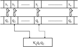
Figure 1: The operating protocol of the composite qubits. For explanation see text.

The generic Hamiltonian of the combined system can be written as $H_{t}=H_{s}+H_{q}+H_{\mathrm{int}}$. Here $H_{s}$ion_trap_decoherence_review describes an harmonically trapped ion manipulated by laser pulses with the motional energy $\hbar\omega_{\nu}\hat{a}^{{\dagger}}\hat{a}$, laser detuning $\delta_{0}\sigma_{z}^{s}$ and the Rabi flipping term $\hbar\omega_{R}\left(\sigma_{+}^{s}e^{i{{}_{l}\delta k_{l}\hat{x}}}+\mathrm{h.c.}\right)$. Here, $\hat{x}$ is the coordinate of the ion, $\hat{a}$($\hat{a}^{\dagger}$) is the lowering(raising) operator, and $\omega_{\nu}$ the trapping frequency. The term $H_{q}=\frac{E_{z}}{2}\sigma_{z}^{q}+\frac{E_{x}}{2}\sigma_{x}^{q}$ describes a solid-state qubit with the generic form of a quantum two level system with energies $E_{x,z}$. The coupling $H_{\mathrm{int}}=\hbar\kappa(t)\hat{x}\sigma_{z}^{q}$ describes a fixed charged particle interacting with a harmonically trapped charged particle. Note the laser pulse generates coupling between the motion $\hat{x}$ of the ion and the internal mode $\sigma_{z}^{s}$ of the ion; hence generates an indirect coupling between the internal mode and the solid-state qubit. The coupling amplitude is of the order of $(\sigma_{z}^{s}\sigma_{z}^{q})Qedr/4\pi\epsilon_{0}r_{0}^{2}$ describing the interaction between a charge $Q$ and a dipole $p_{i}=edr$ with distance $r_{0}$. While for two trapped ions with a distance $r_{0}$, the interaction by laser induced displacements $dr$ is $2(\sigma_{z1}^{s}\sigma_{z2}^{s})e^{2}dr^{2}/r_{0}^{3}$. The interaction between the charge and the ion is hence a factor of $r_{0}/2dr$ stronger than the familiar dipole-dipole couplings encountered in quantum optics, as is shown in Fig. 2 (a) and (b).

Figure 2: The interactions: (a) dipole-dipole interaction between two ions with distance $r_{0}$ and laser induced spatial displacement $\pm d_{r}$ for the internal states $|\uparrow\rangle$ and $|\downarrow\rangle$ respectively; (b) dipole-charge interaction between an ion and a fixed charge; (c) dipole-charge interaction mediated by a metallic connection with a distance $d_{i}$ between the ion and the connection.

2.2 Realization of the Superconducting Qubit

In our previous paperinterfacing , we showed that the hybrid qubit can be formed by connecting an ion with a superconducting charge qubit, i.e. a superconducting island connected to a high resistance tunnel junctions (see Fig. 3). In the charge qubit, the quantum two level system is made of the charge states $|0\rangle=|n\rangle$ and $|1\rangle=|n+1\rangle$, with $n$ the number of Cooper pairs on the island, and the Hamiltonian is $H_{q}$ with $E_{x}=E_{J}$, the Josephson energy, and $E_{z}=E_{c}(C_{g}V_{g}/2e)$, the charge bias due to gate voltage $V_{g}$ and charging energy $E_{c}$superconducting_qubits . Other solid-state systems such as a double quantum dot qubit can be considered within similar framework. Instead of a direct coupling of the ion to the charge qubit, we introduce a superconducting cavity between them, which increases the coupling and provides shielding of the charge qubit from the stray photons of the trap. The cavity is characterized by the capacitance $C_{r}$ and the inductance $L_{r}$ of the cavity, and has eigenfrequencies $\omega_{n}=n/\sqrt{C_{r}L_{r}}$, with $n$ an integer. In our scheme the cavity is much shorter than the microwave wavelength, so that the cavity can be described as two phase variables $\psi_{1,2}$ corresponding to the phases at the ends of the cavity. At one end, the cavity as part of the trap electrode couples with the ion. At the other end, the cavity couples with the charge qubit via the capacitance $C_{m}$. The Lagrangian of the connected system is

$$\begin{array}[]{rcl}\mathcal{L}&=&\displaystyle\frac{C_{r}}{4}\left(\dot{\psi}_{1}^{2}+\dot{\psi}_{2}^{2}\right)+\sum_{k=i.i2}\frac{C_{k}}{2}(V_{k}-\dot{\psi}_{1})^{2}-\frac{(\psi_{1}-\psi_{2})^{2}}{2L_{r}}\\ &+&\displaystyle\frac{C_{t}}{2}\dot{\varphi}^{2}-C_{g}V_{g}\dot{\varphi}-E_{J}\cos{(2e\varphi/\hbar)}+\mathcal{L}_{ion}\\ &+&\displaystyle\frac{C_{m}}{2}(\dot{\psi}_{2}-\dot{\varphi})^{2}+(V_{i}-\dot{\psi}_{1})\frac{e\hat{x}}{d_{i}}\end{array}$$ (1)

where the first line describes the cavity modes with coupling to the voltages $V_{i}$ and $V_{2}$ of the trap electrodes via capacitance $C_{i}$ and $C_{i2}$. The second line describes the charge qubit and the ion with $C_{t}=C_{J}+C_{g}$. The third line is the capacitive couplings between the cavity, the ion and the charge qubit, with $d_{i}$ the distance between the trap electrodes.

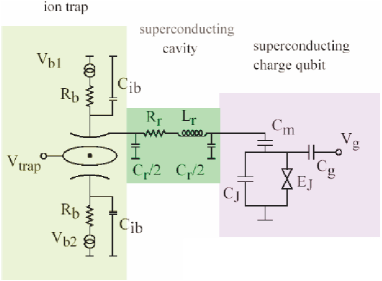
Figure 3: Schematic circuit of the system: ion trap, superconducting cavity and charge qubit.

After integrating out the cavity modes, the effective coupling is interfacing

$$H_{int}^{(2)}=\frac{e^{2}}{C_{\Sigma}}\frac{C_{m}}{C_{t}}\sigma_{z}^{q}\frac{\hat{x}}{d_{i}}$$ (2)

where $C_{\Sigma}\approx C_{r}$ when $C_{r}\gg C_{m},C_{i},C_{t}$. By inserting the cavity, the coupling strength increases by a factor of $10L/d_{i}$ with $10$ a geometry factor, as shown in Fig. 2 . Typical parameters are: cavity length $L=40\,\mathrm{\mu m}$, $C_{r}=3\times 10^{-15}\,\mathrm{F}$, $L_{r}=3\times 10^{-13}\,\mathrm{H}$, $C_{m}=10^{-16}\,\mathrm{F}$, $C_{J}=10^{-16}\,\mathrm{F}\sim C_{g}$, $E_{c}=100\,\mathrm{GHz}$, $e^{2}/2C_{r}=10\,\mathrm{GHz}$, $\omega_{\nu}=1\,\mathrm{MHz}$, and $d_{i}=20\,\mathrm{\mu m}$. With a laser induced separation of $\langle\hat{x}\rangle=\pm 200\,\mathrm{nm}$, $H_{int}^{(2)}=2\pi\times 200\,\mathrm{MHz}$. This interaction results from electrostatic coupling between the cavity, the ion and the charge qubit. Hence no resonance condition between the trap, the cavity and the charge qubit is required and no effort is needed to tune the various systems to match each other.

2.3 Two Qubit Gate

A controlled phase gate $U=e^{-i\left(\pi/4\right)\sigma_{z}^{s}\sigma_{z}^{q}}$ can be performed on the ion and the charge qubit. Three phase gates together with single qubit gates form the swap gate between the two qubitsNielsen_Chuang_book which exchanges the states of the qubits and is the key step in interfacing the ion and the charge qubit. Here it is shown the phase gate does not depend on the initial state of the motion and operates at nanosecond time scale, much shorter than the trapping period $\omega_{\nu}^{-1}$juanjo_fast_gate . We define the free evolution as $U_{0}(t)=\exp{(-i\omega_{\nu}t\hat{a}^{\dagger}\hat{a})}$, the entanglement between the internal mode and the motional mode as $U_{l}(z_{l}n_{l})=\prod_{m=1}^{n_{1}}\\ \sigma_{x}^{s}\exp{(-iz_{m}\delta k_{l}\sigma_{z}^{s}\hat{x})}$ achieved by applying laser $\pi$ pulse for $n_{l}$ times with $z_{m}=(-1)^{m-1}$ and $\delta k_{l}$ the photon momentum, and the entanglement between the charge qubit and the motional mode as $U_{2}(\tau_{q})=\exp{(-iH_{int}^{(2)}\tau_{q}/\hbar)}$ achieved by turning on the capacitive coupling and decreasing the Josephson energy $E_{J}$.

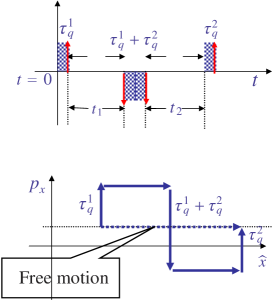
Figure 4: The fast quantum phase gate. Top: the pulse sequence of the gate. Arrow: laser pulse; square: coupling between charge and ion over a time of $\tau_{q}^{1}$, and $\tau_{q}^{1}+\tau_{q}^{2}$ and $\tau_{q}^{2}$, and $t_{1}$ and $t_{2}$: free evolution. Bottom: the phase space evolution of the motional mode under the kicks at qubit states $\sigma_{z}^{q}=\sigma_{z}^{s}=1$. Dotted line is the free evolution.

The gate sequence as is shown in Fig. 4 contains eight steps with three laser kicks of $\left\{n_{l}^{1},-n_{l}^{1}-n_{l}^{2},n_{l}^{2}\right\}$ and three couplings with charge qubit of durations of $\left\{\tau_{q}^{1},-\tau_{q}^{1}-\tau_{q}^{2},\tau_{q}^{2}\right\}$ respectively. These interactions are separated by free evolutions of durations of $t_{1}$ and $t_{2}$. When $n_{l}^{1}t_{1}=n_{l}^{2}t_{2}$ and $\tau_{q}^{1}t_{1}=\tau_{q}^{2}t_{2}$, we have

$$U(T)=e^{i\phi^{\prime}}U_{0}(T)\exp{\left(-i\frac{e^{2}\delta k_{l}\tau_{q}^{1}n_{l}^{1}t_{1}t_{2}}{2C_{r}md_{i}^{2}(t_{1}+t_{2})}\sigma_{z}^{q}\sigma_{z}^{s}\right)},$$ (3)

at $\omega_{\nu}t\ll 1$, with a fidelity of $1-O(\omega_{\nu}^{2}t^{2})$ (Eq. (3) is exact for free particle). It can be showninterfacing that the speed of the phase gate is essentially limited by the laser power and the coupling between the ion and the charge qubit. For the phase gate of $\alpha=\pi/4$, with $t_{1}=t_{2}=5\,\mathrm{nsec}$, $\delta k_{l}=10^{8}\,\mathrm{m}^{-1}$, and $n_{l}^{1,2}=10$, the gate time is $T=14\,\mathrm{nsec}$ for ${{}^{9}}\mathrm{Be}^{+}$ and $T=26\,\mathrm{nsec}$ for ${}^{43}\mathrm{Ca}^{+}$.

3 Decoherence

In quantum computing, it is important that the qubits remain in coherent superposition of the quantum states. Many environmental factors can destroy the coherence of a quantum system. In the hybrid qubit, noise of both qubits and of the connecting circuit causes decoherence. In this section, we study two major sources of decoherence: the charge fluctuations of the solid-state qubit and the cavity dissipation due to the stray photons.

3.1 Charge Fluctuations

In solid-state qubits, one major noise source is charge fluctuations in the substrate or in the gate electrodes due to the imperfections in fabrication. The charge fluctuations can be described as dipole jumps in defects which interacts with the qubit or as charge hoppings near gates which induces image charge on the gate. Due to interaction with their environments, the hopping and the dipole jump occur with a $1/f$ dependent spectrum and cause nonequilibrium and non-Markovian noise to the charge qubit. It has been shown that the decoherence of the charge qubit is dominated by this noise with a decoherence time shorter than nanoseconds when the qubit is away from the degenerate pointnakamura_1_f . In the superconducting charge qubit, the main contribution of the charge noise spectrum is below MHz.

In the hybrid qubit scheme during the storage time, the charge qubit is static at the degenerate point with a bias voltage $V_{g}=0$ and $E_{J}\sim 10\,\mathrm{GHz}$: $H_{q}=E_{J}\sigma_{z}^{q}/2$. Hence the Josephson energy protects the charge qubit from charge fluctuations, and the decoherence time approaches microseconds. However one key step in the controlled phase gate is the evolution $U_{2}(\tau_{q})$ which requires that the charging bias is much stronger than the Josephson energy $\bar{E}_{z}=E_{c}\left(C_{g}\bar{V}_{g}/2e\right)\gg\bar{E}_{J}$, where $\bar{E}_{J}$ is the reduced Josephson energy during the phase gate with $\bar{E}_{J}\sim 100\mathrm{MHz}$ and $E_{J}\gg\bar{E}_{J}$. As a result, the charge qubit is exposed to charge fluctuations in the environment and subject to strong decoherence during the phase gate. The quantum phase gate is performed on a time scale of $20\,\mathrm{nsec.}$ This indicates that charge noise will induce serious decoherence to the system.

The charge fluctuations $\delta Q_{g}$ can be expressed as a voltage noise with $\delta Q_{g}=C_{g}\delta V_{g}$. Adding the voltage noise to the Hamiltonian, we have: $H_{q}=E_{c}\left(C_{g}\bar{V}_{g}+C_{g}\delta V_{g}\right)/2e+\bar{E}_{J}\sigma_{z}^{q}/2$ where the dynamics of the $\bar{E}_{J}$ term, being reduced during the gate, will be neglected in the following discussion. The noise $\delta V_{g}$ is a stochastic operator with a spectrum $\delta V_{\omega}^{2}=2\pi\langle\delta V\left(\omega\right)\delta V\left(\omega^{\prime}\right)\rangle\delta\left(\omega+\omega^{\prime}\right)$ and $\delta V\left(\omega\right)=\int dt^{\prime}e^{i\omega t^{\prime}}\delta V\left(t\right)$, determined by the environment. The low frequency noise has $\delta V\left(\omega\right)\propto 1/\omega$. The gate transformation in Eq. (3) is now

$$U(T)=e^{i\phi^{\prime}}U_{0}(T)e^{-i\bar{E}_{z}T^{\prime}/\hbar}e^{-i\sigma_{z}\phi_{v}\left(t\right)}e^{-i\alpha\sigma_{z}^{q}\sigma_{z}^{s}}$$ (4)

where two phase factors are added compared with Eq.(3): the dynamical phase $e^{-i\bar{E}_{z}T^{\prime}}$ due to the voltage bias in the Hamiltonian; and the stochastic phase $e^{-i\phi_{v}\left(t\right)}$ due to the charge noise. We have $\phi_{v}\left(t\right)=$ $\left(E_{c}C_{g}/2e\hbar\right)\int_{0}^{t}dt^{\prime}$ $\delta V_{g}\left(t^{\prime}\right)$. The dynamical phase does not affect the gate, but the stochastic phase causes serious decoherence.

In the following we extend the quantum phase gate in interfacing and present a scheme that overcomes the effect of the low frequency noise. Instead of directly applying the eight steps of the phase gate, we divide the gate into shorter pieces to improve its resistance to the charge noise. Let $\tau=T/N$ be the unit of improved gate, with $N\gg 1$ being an even integer. The gate consists of $N$ pieces each contributing a phase $\alpha=\pi/4N$ to the quantum phase gate. The gate sequence is now $U(T)=(\sigma_{x}^{q}U(\tau))^{N}$, where after each interval $\tau$, a $\pi$ pulse is applied to the charge qubit to flip the charge state. We assume $\tau$ is of the order of or below nanoseconds. The $\pi$ pulses can be achieved by increasing the effective Josephson energy $\bar{E}_{J}$ to about $10\,\textrm{GHz}$ for short intervals of subnanoseconds; the fidelity of the $\pi$ pulses is mainly limited by the switching time of the Josephson energy and hence the switching time of the flux in the qubit circuit.

The gate evolution is

$$U\left(t\right)=e^{i\phi^{\prime}}e^{i\sigma_{z}\bar{\phi}\left(t\right)}U_{0}(T)e^{-i\frac{\pi}{4}\sigma_{z}^{q}\sigma_{z}^{s}}$$ (5)

where instead of the phase $\phi_{v}\left(t\right)$, the random phase becomes $\bar{\phi}\left(t\right)=\left(E_{c}C_{g}/2e\right)\int dt^{\prime}\delta V_{g}\left(t^{\prime}\right)\,g\left(t\right)$ with

$$g\left(t\right)=\{\begin{array}[]{clc}1,&t\in\left[2n\tau,2n\tau+\tau\right),&\\ -1,&t\in\left[2n\tau+\tau,\left(2n+1\right)\tau\right).&\\ \end{array}$$

which is created by the periodic charge flips. Mathematically, the function $g\left(t\right)$ can be decomposed into triangular functions: $g\left(t\right)=\sum_{m}\left(4/\pi m\right)\sin\omega_{m}t$ with frequencies $\omega_{m}=m\left(2\pi/\tau\right)$ – multiples of $\omega_{1}=2\pi/\tau$. This procedure is equivalent to shifting the noise spectral density of the charge fluctuations by frequencies $\omega_{m}$. In the lowest order, the decoherence rate can be calculated by

$$\gamma_{v}=\frac{\partial\langle e^{i\bar{\phi}(t)}\rangle}{\partial t}\quad\mathrm{and}\quad\langle e^{i\bar{\phi}(t)}\rangle=e^{-\frac{\langle\bar{\phi}^{2}(t)\rangle}{2}}.$$

We have

$$\begin{array}[]{c}\displaystyle\left\langle\bar{\phi}^{2}\left(t\right)\right\rangle_{ev}=\left(\frac{E_{c}C_{g}}{2e}\right)^{2}\frac{4}{\pi^{2}}\sum_{n,m}\frac{1}{mn}\cdot\\ \displaystyle\int\frac{d\omega}{2\pi}\delta V_{\omega}^{2}\int_{0}^{t}dt^{\prime}e^{it^{\prime}\left(\omega_{n}-\omega\right)}\int_{0}^{t}dt^{\prime\prime}e^{-it^{\prime\prime}\left(\omega_{m}-\omega\right)}.\end{array}$$ (6)

Consider $\omega_{1}t\gg 1$. The variance of the random phase is

$$\displaystyle\left\langle\bar{\phi}\left(t\right)^{2}\right\rangle_{ev} = \displaystyle\left(\frac{E_{c}C_{g}}{2e}\right)^{2}\frac{2}{\pi^{2}}\sum_{n}\frac{\delta V_{\omega_{n}}^{2}}{n^{2}}t$$

$$\leq \displaystyle\left(\frac{E_{c}C_{g}}{2e}\right)^{2}\frac{1}{3}\delta V_{\max}^{2}t$$

where in the inequality relation, we replace the spectral density by the maximal spectral density above $\omega_{1}$ ($\omega_{1}\geq\mathrm{GHz}$), and applying the relation: $\sum_{1}^{\infty}1/n^{2}\newline =\pi^{2}/6$. This shows that the decoherence rate is now dominated by noise spectral density above GHz: $\gamma_{v}\leq\left(E_{c}C_{g}/2e\right)^{2}\left(1/3\right)\delta V_{\max}^{2}$, and effect of the low frequency noise is reduced by the charge flips. Note at GHz frequencies, the charge noise is mainly thermal noise of the connecting circuits, e.g. Johnson-Nyquist noise of the resistances in the circuit. In experiments, this noise induces a decoherence rate slower than MHzSaclay_exp . By flipping the charge qubit at very short intervals $m\tau$, a spin-echo type of spectral modulation is achieved which engineers the noise spectral density and hence protects the charge qubit from the low frequency noise.

In a scalable scheme, to avoid affecting other charge qubits by the fast flips of one qubit, we consider using local superconducting wire to control the flux in the double junction of the charge qubitsuperconducting_qubits . Because the flux generated by a wire decreases with the distance to the wire $r$ as $1/r$, only nearby charge qubits will be affected by this flux. Meanwhile, we design the charge biases $E_{c}(C_{g}V_{g}/2e)$ of the qubits in a neighborhood to have differences above $5\,\mathrm{GHz}$. With a flipping rate of GHz, the off resonance in the other qubits will prevent their flipping.

3.2 Cavity Dissipation

Another source of decoherence we consider is the losses in the superconducting cavity which introduces decoherence to the qubits. At low temperature in a superconductor, the quasiparticle density decreases exponentially with temperature: $n_{n}=n_{0}\exp{(-2\Delta/k_{B}T)}$, so that the dissipation due to quasiparticle conduction can be neglected. However, when laser photons, e.g. from the laser driven ion, are scattered to the superconductor, quasiparticles are excited and dissipation increases. In our previous paperinterfacing , we estimated the effect of the induced quasiparticles on decoherence. Here, we present a path integral approach to calculate the decoherence rate.

We model the dissipation of the cavity as a resistor in series with the cavity inductance. The resistance is $R_{r}=R_{n}(n_{ex}/n_{0})$jackson_em ; tinkham_superconductivity , where $R_{n}$ is the normal state resistance of the superconductor. Considering a laser power of mW, and assume the stayed photons consist $10^{-6}$ of the laser power. In a duration of $100\,\mathrm{nsec}$, the photons excite quasiparticles that can be modeled as a resistance of $R_{r}=R_{n}/10^{5}$.

The dissipation can be calculated with the standard Caldeira-Leggett formalismgrabert_phys_rep which treats the environments as an oscillator bath that couples with the qubit linearly. We derive the effective spectral density of the cavity resistance. The Hamiltonian including the bath and the cavity modes is

$$H_{R}=H_{cav}+\tilde{\psi}_{k}\sum_{j}\lambda_{j}x_{j}+\sum_{j}\left(\frac{p_{j}^{2}}{2m_{j}}+\frac{m_{j}\omega_{j}^{2}}{2}x_{j}^{2}\right)$$ (7)

where $H_{cav}$ is the cavity Hamiltonian derived from Eq.(1); $x_{j}$s are the coordinates of the oscillator modes in the bath, $p_{j}$s are the momenta of the oscillator modes, $m_{j}$s the mass, $\omega_{j}$s the oscillator frequencies, with the last term being the Hamiltonian of the bosonic modes. The couplings between the oscillators and the cavity mode $\tilde{\psi}_{k}$ are the $\lambda_{j}$s which determine the noise spectral density $J_{0}(\omega)=\sum\lambda_{j}^{2}/2m_{j}\omega_{j}\delta(\omega-\omega_{j})$. In the case of a resistance, we have $J_{0}(\omega)=\omega R_{r}^{-1}$. Note the complete Hamiltonian is $H_{t}+H_{R}$ including the ion, the charge qubit, the cavity and the bath. In the path integral approach, the harmonic oscillator degrees of freedom can be integrated exactly as we are only concerned with the dynamics and decoherence of the qubits. In the following we take the charge qubit as an example to study the decoherence. The same approach can be applied to the motion of the ion. After integrating out both the cavity and the bath modes, the effective action of the charge qubit is

$$\begin{array}[]{c}\displaystyle S_{eff}^{E}[\bar{\varphi}]=\int_{0}^{\hbar\beta}d\tau\frac{C_{t}}{2}\dot{\varphi}^{2}-E_{J}\cos{(2e\varphi/\hbar)}\\ \displaystyle+\frac{1}{2}\int_{0}^{\hbar\beta}d\tau\int_{0}^{\hbar\beta}d\sigma k(\tau-\sigma)\dot{\varphi}(\tau)\dot{\varphi}(\sigma)\end{array}$$ (8)

where $\varphi$ is the gauge invariance phase of the charge qubitgrabert_phys_rep , and $\beta=1/k_{B}T$ with $T$ being the temperature. The function $k$ is

$$k(\tau)=-\frac{(C_{m}/2C_{t})^{2}}{\hbar\beta(C_{r}+C_{m})}\sum_{n=-\infty}^{+\infty}\frac{\nu_{n}^{2}e^{i\nu_{n}\tau}}{(\nu_{n}^{2}+\omega_{r}^{2}+|\nu_{n}|\hat{\gamma}(|\nu_{n}|))},$$ (9)

with $\omega_{r}=2/\sqrt{(C_{r}+C_{m})L_{r}}$ and $\nu_{n}=2\pi n/\hbar\beta$ being the Matsubara frequencies at integer $n$. Let the Fourier transformation of $k(\tau)$ be $\widetilde{k}(i\nu_{n})=\int_{0}^{\hbar\beta}d\tau k(\tau)\exp{(i\nu_{n}\tau)}$. The retarded noise spectral function is

$$\widetilde{k}(i\nu_{n}=\omega+i\delta)=(\frac{C_{m}}{2C_{t}})^{2}i\omega Z_{\mathrm{eff}}(\omega)$$ (10)

where the spectral density is characterized by an effective impedance $Z_{\mathrm{eff}}$ described as a capacitor $(C_{r}+C_{m})/4$ in parallel to the series of the inductor $L_{r}$ and the resistor $R_{r}$. When $\omega\ll 1/\sqrt{L_{r}C_{r}}$, we have $Z_{\mathrm{eff}}\approx R_{r}$.

The action in Eq. (8) describes the charge qubit interacting with a fluctuating field with a spectral density

$$\begin{array}[]{c}\displaystyle J_{\mathrm{eff}}\left(\omega\right)=\mathrm{Im}[\widetilde{k}(\omega+i\delta)]\\[5.69054pt] \displaystyle=(\frac{C_{m}}{2C_{t}})^{2}\omega Z_{\mathrm{eff}}(\omega)\coth\left(\frac{\hbar\omega}{2k_{B}T}\right)\end{array}$$ (11)

which is derived from the above discussion. The decoherence rate of the charge qubit $\gamma_{r}^{q}$ can be derived from $J_{\mathrm{eff}}\left(\omega\rightarrow 0\right)$ according to the fluctuation dissipation theorem:

$$\gamma_{r}^{q}\approx\frac{R_{r}}{R_{k}}\frac{2k_{B}T}{\hbar}(\frac{C_{m}}{2C_{t}})^{2}$$ (12)

where $R_{k}=\hbar/(2e)^{2}$ is the quantum resistance. At a temperature of $T=100\,\mathrm{mK}$, we have $\gamma_{r}^{q}=50\,\mathrm{msec}^{-1}$. This shows that the dominant decoherence is not due to the cavity losssuperconducting_qubits ; ion_trap_exp_review_wineland , but most likely due to the charge noise.

4 Experimental Issues

Combining systems as different from each other as the ion trap and the solid-state qubit is a challenge for existing experimental techniques. Questions arise such as whether the two systems are compatible and whether the techniques developed for a conventional system can be applied to the combined system. In this section we investigate several experimental issues of the combined system, including the fast switch during the swap gate, the balance circuit that decouples the charge qubit from the ac driving of the trap and the scalability issue.

4.1 Fast Switch

In the quantum phase gate, the laser pulse, the coupling between the ion and the charge, and the free evolution are applied alternatively, which requires a fast switch that can turn on and turn off the capacitive coupling in a time scale shorter than the gate timeinterfacing . Various switch circuits have been studied with mesoscopic electronics such as the superconducting field effect transistor, superconducting single electron transistor, and the $\pi$-junctions of high T_c materialssuperconducting_qubits . In this section we study a fast electronic switch made of dc SQUID.

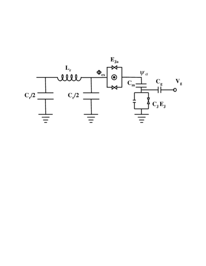
Figure 5: Schematic circuit of superconducting dc SQUID switch inserted between the cavity and the charge qubit. The island between the switch and the capacitor $C_{m}$ is labeled $\psi_{a}$.

The switch, inserted between the superconducting cavity and the capacitor $C_{m}$ is shown in Fig. 5. The switch is made of two large Josephson junctions with a Josephson energy $E_{Ja}$ much larger than the Josephson energy $E_{J}$ of the charge qubit forming a dc SQUID, and the charging energy of the junctions is negligible. In the dc SQUID geometry, the switch is described as a junction with an effective Josephson energy $E_{a}=2E_{Ja}\cos{(\mathrm{\pi\Phi_{ex}/\Phi_{0}})}$ depending on the external flux $\mathrm{\Phi_{ex}}$ in the SQUID loop, with $\mathrm{\Phi_{0}}$ the flux quantum. This shows that when $\mathrm{\Phi_{ex}=\Phi_{0}/2}$, the connection between the cavity and the charge qubit is cut off by the SQUID. Below, we derive the coupling between the charge qubit and the ion in the presence of the switch.

We introduce four phase variables to describe the circuit in Fig. 5: $\psi_{1,2}$ of the left and the right ends of the cavity, $\psi_{a}$ of the island between the switch and the capacitor $C_{m}$, and $\varphi$ of the charge qubit. The Lagrangian of the system can be derived by replacing the term $C_{m}(\dot{\psi}_{2}-\dot{\varphi})^{2}/2$ in Eq. (1) with

$$\frac{C_{m}}{2}(\dot{\psi}_{a}-\dot{\varphi})^{2}+E_{a}\cos{(\frac{2e(\psi_{2}-\psi_{a})}{\hbar})}$$ (13)

which includes the capacitive energy of $C_{m}$ and the Josephson energy of the SQUID. The Hamiltonian can be derived as:

$$\begin{array}[]{ccl}\displaystyle H_{sw}&=&\displaystyle\frac{p_{1}^{2}+p_{2}^{2}}{C_{r}}+\frac{2p_{1}e}{C_{r}}\frac{\hat{x}}{d_{i}}+\frac{(\psi_{1}-\psi_{2})^{2}}{2L_{r}}+\frac{p_{a}^{2}}{2C_{a}}\\[5.69054pt] &\displaystyle+&\displaystyle\frac{(p_{\varphi}+C_{g}V_{g})^{2}}{2C_{t}}-E_{J}\cos{(2e\varphi/\hbar)}\\[5.69054pt] &\displaystyle+&\displaystyle\frac{p_{a}(p_{\varphi}+C_{g}V_{g})}{C_{t}}-E_{a}\cos{(\frac{2e(\psi_{2}-\psi_{a})}{\hbar})}\end{array}$$ (14)

where $p_{i},\,i=1,2,a,\varphi$ are the conjugate variable of the corresponding phase variables and $C_{a}=C_{m}C_{t}/(C_{m}+C_{t})$. Here the charging energy of the island between the switch and $C_{m}$ is $p_{a}^{2}/2C_{a}$, and the last two terms are the coupling between $p_{a}$ and the cavity, and the coupling between $\psi_{a}$ coupling and the charge qubit. When $\cos{(\mathrm{\pi\Phi_{ex}/\Phi_{0}})}=0$, i.e. $\mathrm{\Phi_{ex}=\Phi_{0}/2}$, the last term in Eq. (14) disappears, and hence the cavity together with the ion is disconnected from the island $\psi_{a}$ and the charge qubit. After integrating out $\psi_{a}$, the charge qubit Hamiltonian is $(p_{\varphi}+C_{g}V_{g})^{2}/2(C_{m}+C_{t})-E_{J}\cos{(2e\varphi/\hbar)}$ consistent with the Hamiltonian without the switch. This shows that the coupling between the charge qubit and the ion can be turned off by applying a $\pi$-flux in the SQUID loop.

Now we calculate the effective coupling between the charge qubit and the ion with the switch on. The large Josephson junction can be modeled as an inductance with $L_{\mathrm{eff}}=(\hbar/2e)^{2}/E_{a}$ and the energy is $(\psi_{2}-\psi_{a})^{2}/2L_{\mathrm{eff}}$. The quadratic Hamiltonian of $\psi_{1,2,a}$ and $p_{1,2,a}$ can be diagonalized into secular modes $\psi_{k}=\sum v_{ki}\psi_{i}$ and $p_{k}=\sum v_{ki}^{\star}p_{i}$ with $i=1,2,a$ and $k=A,B,C$. One of these modes $\psi_{C}$ is $\psi_{C}=\sum\psi_{i}/\sqrt{3}$ with $p_{C}=\sum p_{i}/\sqrt{3}$ and the secular value zero. Fig. 5 shows that $p_{C}=0$. Hence we derive:

$$\begin{array}[]{ccl}\displaystyle H&\displaystyle=&\displaystyle\sum_{k=A,B}\frac{p_{k}^{2}}{C_{r}}+\frac{\psi_{k}^{2}}{2L_{k}}+\frac{(p_{\varphi}+C_{g}V_{g})^{2}}{2C_{t}}-E_{J}\cos{(2e\varphi/\hbar)}\\[8.53581pt] &\displaystyle+&\displaystyle\sum_{k=A,B}2p_{k}\left(\frac{e\hat{x}}{d_{i}}v_{k1}+\frac{\sqrt{C_{r}C_{a}}(p_{\varphi}+C_{g}V_{g})}{\sqrt{2C_{t}}}v_{k3}\right)\end{array}$$ (15)

where $L_{A,B}$ are functions of $L_{r}$ and $L_{\mathrm{eff}}$ and are the other two secular values besides zero. Integrating $\psi_{A,B}$, the effective interaction between the charge qubit and the ion is $H_{int}^{sw}=(e^{2}C_{m}\hat{x}/C_{r}C_{t}d_{i})\sigma_{z}^{q}$, exactly the same as that in Eq. (2). At the same time, the integration also gives a correction to the charge qubit which recovers the form of $(p_{\varphi}+C_{g}V_{g})^{2}/2(C_{m}+C_{t})$. This shows that by inserting a switch with $\hbar/\sqrt{L_{\mathrm{eff}}C_{r}}\gg E_{J}$, the coupling strength is not affected; while when the critical current disappears, the coupling disappears as well.

The performance of switch is limited by the speed of switching the flux $\Phi_{ex}$ in the SQUID and by the incomplete turning off of the switch. This may be overcome by inserting a $\pi$-junction into the circuit instead of applying magnetic fluxsuperconducting_qubits . In practice, the large junctions of the SQUID couple with flux noise or current noise, and may bring decoherence to the circuit. The decoherence of various switches was studied in storcz_wilhelm .

4.2 The Balance Circuit

In standard ion traps, electromagnetic fields are applied to achieve trapping of the ions. For example, in a Paul trap, typically an ac voltage of 100 – 250 MHz and 30 – 50 Volts is applied on the electrodes; in a Penning trap, a magnetic field gradient is applied. The coupling between the ion and the charge qubit not only brings interaction between the two qubits, but also connects the driving fields with the charge qubit. However, the superconducting charge qubit can not coexist with strong external fields. Here we show that the external field can be canceled by designing a balance circuit.

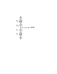
Figure 6: The balance circuit. The ac voltages $V_{i}$ and $V_{ib}$ are applied to the trap electrodes. This circuit is connected to the superconducting cavity.

We consider a Paul trap connecting with the superconducting cavity. As is shown in Fig. 6 and described by the $\sum C_{k}(V_{k}-\dot{\psi_{1}})^{2}/2$ term in Eq. (1), the cavity is part of the electrodes and is coupled to the driving voltages via the capacitors $C_{k}$. These couplings contribute to the Hamiltonian as

$$\frac{e^{2}}{C_{\Sigma}}\frac{C_{m}}{C_{t}}\frac{(C_{i}V_{i}+C_{ib}V_{ib})}{e}\sigma_{z}^{q}$$ (16)

and can have significant influence on the charge qubit. However, by choosing the balance condition $C_{i}V_{i}+C_{ib}V_{ib}=0$, this coupling disappears, and the charge qubit is protected in an experiment. The balance condition discussed above can only be achieved approximately due to the inaccuracy in the controlling of the voltages. With an inaccuracy of $10^{-4}\,\mathrm{V}$ in the voltage sources, and $C_{i}\sim C_{t}/10$ ($d_{i}=20\,\mathrm{\mu m}$ and area of electrodes $10^{-12}\,\mathrm{\mu m}^{2}$), the coupling of the voltage sources with the charge qubit $\delta E\sigma_{z}^{q}$ is $\delta E=100\,\mathrm{MHz}$, much less than the charging energy $e^{2}/C_{r}$ and the coupling in Eq. (2). In addition, the frequencies of the driving voltages is around 100 – 200 MHz, much less than the charge qubit energy; hence this inaccuracy and moreover the coupling between the charge qubit and the driving voltages does not bring serious effect on the charge qubit.

4.3 Scalability

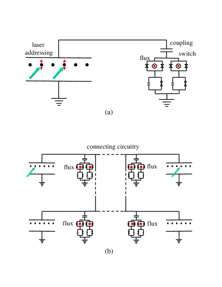
Figure 7: Top: an array of ions in a linear trap couple with the charge qubits via the cavity. Bottom: four hybrid systems couple with each other via superconducting transmission line or capacitive coupling (dash lines represent the coupling circuit).

With the hybrid system, we hope to achieve scalable quantum computing without moving ions. To exploit the advantages of both the ion and the charge qubit, we consider the scheme shown in Fig. 7 as an example. Compared with pure ion trap qubits, it is harder to fabricate large numbers of the hybrid qubits which consist of an ion and a charge qubit each. Instead, we design the hybrid system in the form of clusters: an array of ions trapped in a linear trap are connected with two charge qubits via a superconducting cavity – a cluster of small numbers of ion qubits. The charge qubits capacitively couple with the cavity, and the couplings are controlled by the switches made of the SQUIDs.

During a controlled phase gate between ions in the same cluster, one ion is addressed by a polarization dependent laser pulse that pushes the ion in the transverse direction which is shown by the arrows in Fig. 7. All the other ions in the array are unaffected. This is followed by turning on the switch of one charge qubit to allow the coupling between the charge qubit and the addressed ion. After the gate sequence in Eq. (3), the phase gate is obtained between this ion and this charge qubit, and subsequenctly the swap gate. For the other ions, the evolution is $U^{\prime}(T)=\exp{(-i\omega_{\nu}t\hat{a}^{\dagger}\hat{a}+i\phi^{\prime\prime})}$ which is nothing but free evolution; hence the other ions are exempted from the controlled gate. The same procedure is then applied to the other ion involved in the controlled gate after which the two qubit gate is performed on the charge qubits. Note when addressing an ion in its transverse direction, the Coulomb interaction between the ions contributes a small force in the same direction of the transverse motion. This force is smaller than the force of the trapping potential when the distance between the ions is longer than microns at a trapping frequency of $10\,\mathrm{MHz}$.

Based on this scheme, multiple clusters of the hybrid system can be fabricated. In Fig. 7, we show four such systems each including an array of ion in the ion trap and two charge qubits. The clusters are coupled by capacitively connecting a charge qubit in one cluster with another charge qubit in another clusters. With superconducting transmission lines, distant qubits with a separation of centimeters can be connected with an interaction strength of $100\,\mathrm{MHz}$Girvin_Schoelkopf . Quantum logic gates on qubits in the same cluster can be performed on the charge qubits in the same cluster. Quantum logic gates on qubits in distant clusters can be performed via the capacitive connections. Note when there are many clusters, connections between neighboring clusters are sufficient to obtain interactions between qubits in any two clusters.

5 Discussions and Conclusion

We studied several issues in the interfacing of ion trap qubits and solid-state charge qubits: decoherence, coupling mechanism, switching of coupling, and scalability. We calculated the decoherence due to the charge noise and the dissipation of the cavity, and presented a gate scheme that can overcome the charge noise. We analyzed a crucial element of this scheme: a fast switch that is made of a dc SQUID and can turn off the coupling between the charge qubit and the ion. We also present an example of scalable hybrid schemes where the ion qubits are aligned in clusters – an array of ions coupling with charge qubits. It is shown from these discussions that the hybrid system is a scalable quantum computing system that may be able to exploit and combine the merits of very different systems. Note we concentrate on a special example of ion trap qubit coupling with superconducting systems. Study on interfacing other systems, e.g. nanomechanical resonator and superconducting qubitcpb_mechanical_resonator_schwab , has been studied.

On the other hand, connecting systems as different as the ion trap and the charge qubit is very challenging. For example, the charge qubits have to work at millikelvin temperature in a dilution fridge. This requires that the ions have to be positioned in the fridge as well. This also brings up the questions of including the laser in the fridge. We analyzed several experimental issues in this paper, such as the balance circuit, the state flipping scheme and the fast switch. Such issues are technically demanding. We would like to point out that the study of hybrid systems is still at the very beginning and some part of the theory is still speculative. While we expect more interest and study on interfacing different systems in near future.

Acknowledgments: Work supported by the Austrian Science Foundation, European Networks and the Institute for Quantum Information.

References

- (1) L. Tian and et al., Phys. Rev. Lett. 92, (2004) 247902.
- (2) F. Schmidt-Kaler and et al., Nature 422, (2003) 408; D. Leibfried and et al., Nature 422, (2003) 412; M. Riebe et al, Nature 429, (2004) 734; M. D. Barrett et al, Nature 429, (2004) 737.
- (3) D. Kielpinski, C. Monroe, and D. J. Wineland, Nature 417, (2002) 709; J. I. Cirac and P. Zoller, Nature 404, (2000) 579.
- (4) J. I. Cirac and P. Zoller, Phys. Today March 57, (2004) 38 ; J. I. Cirac and P. Zoller, Phys. Rev. Lett. 74, (1995) 4091.
- (5) Y. Makhlin, G. Schön, and A. Shnirman, Rev. Mod. Phys. 73, (2001) 357; J.E. Mooij and et al., Science 285, (1999) 1036; Yu. A. Pashkin and et al., Nature 421, (2003) 823; I. Chiorescu and et al., Science 299, (2003) 1869.
- (6) D. Loss and D. P. DiVincenzo, Phys. Rev. A 57, (1998) 120; W. G. van der Wiel and et al., Rev. Mod. Phys. 75, (2003) 1.
- (7) D. P. DiVincenzo, in Fortsch. Phys. vol 48, special issue on Experimental Proposals for Quantum Computation (2000), also available at quant-ph/0002077.
- (8) See also: A. D. Armour, M. P. Blencowe, and K. C. Schwab, Phys. Rev. Lett. 88, (2002) 148301.
- (9) D.J. Heinzen and D.J. Wineland, Phys. Rev. A 42, (1990) 2977.
- (10) D. Leibfried and et al, Rev. Mod. Phys. 75, (2003) 281.
- (11) A. J. Leggett, Phys. Rev. B 30, (1984) 1208; S. Chakravarty and A. Schmid, Phys. Rev. B 33, (1986) 2000.
- (12) M. A. Nielson and I. L. Chuang, Quantum Computation and Quantum Information, (Cambridge University Press, 2000).
- (13) J. J. Garcia-Ripoll, P. Zoller, and J. I. Cirac, Phys. Rev. Lett. 91, (2003) 157901.
- (14) Y. Nakamura, Yu. A. Pashkin, T. Yamamoto, and J. S. Tsai, Physica Scripta 102, (2002) 155; Y.M. Galperin, B.L. Altshuler and D.V. Shantsev, cont-mat/0312490.
- (15) D. Vion et al., Science 296, (2002) 886.
- (16) J.D. Jackson, Classical Electrodynamics,(John Wiley & Sons, Inc, 1975, 2nd ed.).
- (17) M. Tinkham, Introduction to Superconductivity, (McGraw-Hill, New York, 1996, 2nd ed.).
- (18) H. Grabert, P. Schramm, and G.-L. Ingold, Phys. Rep. 168, (1988) 115; L. Tian, S. Lloyd and T.P. Orlando, Phys. Rev. B. 65, (2002) 144516.
- (19) D. J. Wineland and et al., J. Res. Natl. Inst. Stand. Technol. 103, (1998) 259.
- (20) M. J. Storcz and F. K. Wilhelm, Appl. Phys. Lett. 83, (2003) 2389; C. Cosmelli and et al., cond-mat/0403690.
- (21) A. Wallraff and et al., Nature 431, (2004) 162; S.M. Girvin and et al., cond-mat/0310670.