Schrödinger Cat States of a Nanomechanical Resonator

Abstract

We present a scheme of generating large-amplitude Schrödinger cat states and entanglement in a coupled system of nanomechanical resonator and single Cooper pair box (SCPB), without being limited by the magnitude of the coupling. It is shown that the entanglement between the resonator and the SCPB can be detected by a spectroscopic method.

The fabrication and probing of ultra-small nanomechanical resonators with secular frequencies of $\mathrm{GHz}$ and quality factors approaching $10^{5}$ have been achieved in recent experimentsResonatorSET . These resonators are promising systems for demonstrating the quantum mechanical nature of the mechanical degrees of freedomNanoResonator . Potential applications include detection of weak forces, precision measurement, and quantum information processingforcedetection ; Munro_measurement ; QIP_resonator . One crucial step in studying the nanomechanical resonators will be the quantum engineering and the detection of the mechanical modes. This can be achieved by connecting the resonators with solid-state electronic devicesResonatorSET ; resonator_SCPB1 ; resonator_SCPB2 , for example coupling a resonator with a single electron transistor (SET) via electrostatic interaction. The SET measures the flexural oscillation of the resonator with an accuracy approaching the quantum limitResonatorSET . Cooling of a resonator to its ground state has been proposed by quantum feedback control via a SETfeedback_cooling and by side band cooling via a quantum dotwilsonrae_cooling or a SCPBResonator_cooling .

The resonator modes can be treated as underdamped harmonic oscillators with the damping described by the finite quality factor $Q$. Connecting a resonator with a quantum two level system forms a spin-oscillator model which has been intensively studied in quantum optics, especially in ion trap quantum computingIonTrap_Rev . Hence the techniques of manipulating the motional state of a trapped ion by laser control of its internal mode can be applied to studying the nanomechanical resonatorsIonTrap_Rev . In Ref. resonator_SCPB1 ; resonator_SCPB2 , the capacitive coupling between a nanomechanical resonator and a SCPB was studied, where the SCPB can be treated as a two level system – the superconducting charge qubit – by adjusting the parameters and the gate voltagecharge_qubit_mss . It was shown that entanglement between the resonator and the qubit can be generated and be detected by interferometry when the coupling is stronger than the energy of the resonator. In this paper, we show that large-amplitude Schrödinger cat states and entanglement can be generated in the coupled resonator and SCPB system by parametric pumping of the SCPB when the magnitude of coupling is weak due to the geometry of the charge island and the distance between the charge island and the resonatorResonator_cooling . Given the large amplitude of the generated cat states, the entanglement between the resonator and qubit can be observed by a spectroscopic measurement which selectively flips the charge qubit depending on the state of the resonator. When the scheme is generalized to two or more nanomechanical resonators, it generates maximal entanglement between these resonators, which is a key element in continuous variable quantum computingqc_braunstein . In precision measurement, the cat state of $N$ resonators can increase the sensitivity to weak forces by a factor of $\sqrt{N}$Munro_measurement . The effect of environmental fluctuations including the mechanical noise and the charge noise around the charge island is analyzed. Furthermore, as this scheme involves the generic system of one spin and one oscillator, it can be tailored for other applications such as single spin detection by a cantileversingle_spin_detection .

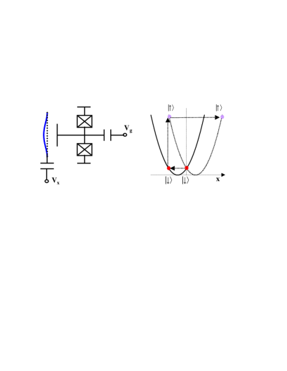
Figure 1: Left: a resonator couples with a SCPB. Right: the trajectory of the resonator starts from the origin $x=0$ (thin dotted line) and the state $|\downarrow\rangle$ of the charge qubit; the qubit is flipped every half period of the resonator $\pi/\omega_{0}$.

The coupled system of a nanomechanical resonator and a SCPB is shown in Fig. 1, with the resonator undergoing flexural vibration. The flexural mode is described by the Hamiltonian $H_{m}=\hbar\omega_{0}\hat{a}^{{\dagger}}\hat{a}$ where $\omega_{0}$ is the frequency of the mode and $\hat{a}^{\dagger}$ ($\hat{a}$) is the raising (lowering) operator of the mode. The resonator is biased at a voltage $V_{x}(t)$ and couples to the SCPB through a capacitance $C_{x}(\hat{x})=C_{x0}(1+\hat{x}/d_{0})$ where $C_{x0}$ is the static capacitance, $d_{0}$ the static distance between the two, and $\hat{x}=\delta x_{0}(\hat{a}+\hat{a}^{\dagger})$ the displacement of the flexural mode with $\delta x_{0}=\sqrt{\hbar/2m\omega_{0}}$ the quantum width of the resonator. The SCPB is a superconducting island connected with Josephson junctions and is controlled by the gate voltage $V_{g}(t)$ through the gate capacitance $C_{g}$. When $C_{g}V_{g}+C_{x}V_{x}=(2n+1)e+2e\delta n$ with $n$ integer and $\delta n\ll 1$, the SCPB can be treated as an effective quantum two level system – the superconducting charge qubitcharge_qubit_mss – described by the Hamiltonian $H_{q}=4E_{c}\delta n\sigma_{z}+\frac{E_{J}(t)}{2}\sigma_{x}$ with $E_{c}=e^{2}/2C_{\Sigma}$ the charging energy, $C_{\Sigma}$ the total capacitance connected with the charge island, and $E_{J}(t)$ the Josephson energy with a small modulation around the static Josephson energy $E_{J0}$. Here $\sigma_{x,z}$ are Pauli operators for the two level system. To the lowest order, the coupling between the resonator and the SCPB is $-\lambda\left(t\right)\left(\hat{a}+\hat{a}^{{\dagger}}\right)\sigma_{z}$ with $\lambda(t)=4E_{c}(V_{x}(t)C_{x0}/2e)(\delta x_{0}/d_{0})$, and its magnitude can be limited by $C_{x0}$ and the small ratio of $\delta x_{0}/d_{0}$. In our scheme, the bias of the resonator is $V_{x}(t)=V_{x0}\cos\left(\omega_{ac}t\right)$, an ac voltage with amplitude $V_{x0}$ and frequency $\omega_{ac}$; the gate voltage is $V_{g}(t)=V_{dc}+V_{g0}\cos\left(\omega_{ac}t\right)$, including a dc voltage $V_{dc}$ and an ac voltage with amplitude $V_{g0}$ and frequency $\omega_{ac}$. We let $C_{g}V_{dc}=(2n+1)e$ so that the charge qubit operates at the degenerate pointoptimal_point . In experiments, it was shown that the decoherence time of the charge qubit at the degenerate point can be as long as microsecondsoptimal_point . Here $\omega_{ac}=E_{J0}/\hbar$ is in resonance with the energy of the charge qubit at the degenerate point. In the following we study the system in the rotating frame of $\frac{E_{J0}}{2}\sigma_{x}$. In this frame the Hamiltonian after the rotating wave approximation can be derived as

$$H_{rot}=\hbar\omega_{0}\hat{a}^{{\dagger}}\hat{a}-\frac{\lambda_{0}}{2}\left(\hat{a}+\hat{a}^{{\dagger}}\right)\sigma_{z}-\frac{\epsilon_{z}}{2}\sigma_{z}+\frac{\epsilon_{\perp}\left(t\right)}{2}\sigma_{x}$$ (1)

where $\lambda_{0}=4E_{c}(V_{x0}C_{x0}/2e)(\delta x_{0}/d_{0})$ is the coupling in the rotating frame, $\epsilon_{z}=8E_{c}(C_{g}V_{g0}+C_{x0}V_{x0})/2e\ll E_{c}$, and $\epsilon_{\perp}=E_{J}(t)-E_{J0}$ is the small modulation of the Josephson energy. Here, the dynamics of the resonator is that of a shifted harmonic oscillator with the Hamiltonian $DH_{m}D^{\dagger}$ with the displacement operator

$$D=\exp\left(-\left(\hat{a}-\hat{a}^{{\dagger}}\right)\frac{\lambda_{0}\sigma_{z}}{2\hbar\omega_{0}}\right).$$

Typical parametersResonator_cooling are $E_{J0}\approx 10\,\mathrm{GHz}$, $E_{c}\approx 50\,\mathrm{GHz}$, $C_{x0}\approx 20\,\mathrm{aF}$, and $\omega_{0}\approx 100\,\mathrm{MHz}$. With $V_{x0}\approx 1\,\mathrm{V}$, the coupling is $\lambda_{0}\approx 20\,\mathrm{MHz}$.

Below we show that by pumping the charge qubit with stroboscopic pulses, Schrödinger cat states with large amplitude can be generated in this system. In an ideal situation, we consider $\delta$-function pulse sequence

$$\epsilon_{\perp}\left(t\right)=\pi\delta\left(n\tau_{0}\right),\quad\mathrm{with}\,n\geq 1,\mathrm{\ \ }\mathrm{integer}$$ (2)

where each pulse is a transformation $-i\sigma_{x}$ that flips the charge qubit after every half period of the resonator mode $\tau_{0}=\pi/\omega_{0}$. Here $\epsilon_{z}=0$. The $\delta$-function approximation is valid when $\epsilon_{\perp}\gg\hbar\omega_{0},\lambda_{0}$. Let $U_{1}=e^{-iH_{rot}\tau_{0}}|_{\epsilon_{\perp}=0}$ be the free evolution of the system between the pulses: $U_{1}=De^{-i\pi\hat{a}^{{\dagger}}\hat{a}}D^{{\dagger}}$. At times $n\tau_{0}$ after the $n$th pulse, the unitary transformation on the system is $U\left(n\tau_{0}\right)=\left(-i\sigma_{x}U_{1}\right)^{n}$. With the relations: $\sigma_{x}D\sigma_{x}=D^{\dagger}$ and $e^{i\pi\hat{a}^{{\dagger}}\hat{a}}De^{-i\pi\hat{a}^{{\dagger}}\hat{a}}=D^{\dagger}$, we derive

$$U\left(n\tau_{0}\right)=\{\begin{array}[]{ll}(D^{\dagger})^{2n},&n\in even\\[5.69054pt] \sigma_{x}e^{-i\pi\hat{a}^{{\dagger}}\hat{a}}(D^{{\dagger}})^{2n},&n\in odd\end{array}$$ (3)

where the overall phase factors are omitted. This transformation generates in the wave function of the resonator a displacement of $\Delta x=-\delta x_{0}\left(2n\lambda_{0}\sigma_{z}/\hbar\omega_{0}\right)$ when $n$ is even, and an opposite displace when $n$ is odd. With the initial state $|\psi_{0}\rangle=(c_{0}|\uparrow\rangle+c_{1}|\downarrow\rangle)\int dx|x\rangle\varphi(x)$, where the states $|\uparrow,\downarrow\rangle$ are eigenstates of the charge qubit in the $\sigma_{z}$ basis and $\varphi(x)$ is the wave function of the resonator, after even number of flips $n$, the state is

$$c_{0}\left|\uparrow\right\rangle\int dx\left|x\right\rangle\varphi(x+\Delta x)+c_{1}\left|\downarrow\right\rangle\int dx\left|x\right\rangle\varphi(x-\Delta x)$$ (4)

where the state of the resonator is shifted according to the state of the charge qubit.

Assume an initial state of $|\psi_{0}\rangle=\frac{1}{\sqrt{2}}(|\uparrow\rangle+|\downarrow\rangle)|0\rangle$ where $|0\rangle$ is the ground state of the resonator and $\lambda_{0}=0$ at $t<0$. Following Eq. (1), after even number of pulses $n$, the state $\frac{1}{\sqrt{2}}(|\uparrow~{}\rangle|-2n\alpha_{0}\rangle+|\downarrow~{}\rangle|2n\alpha_{0}\rangle)$ is generated where $\alpha_{0}=\lambda_{0}/2\hbar\omega_{0}$ is the dimensionless coupling. The state $|\alpha\rangle$ denotes a coherent state of the resonator mode with an amplitude $\alpha$. When $2n\alpha_{0}\gg 1$, maximal entanglement is generated between the resonator and the charge qubit. An intuitive way to describe the process is to consider a classical particle with two spin components in an harmonic potential, where the potential is shifted from the origin to the left (right) at spin down (up) when the coupling is on. The spin is subject to kicks every half period of the oscillator, as shown in Fig. 1. At $t<0$, the oscillator is at the origin in its ground state with no coupling. At $t>0$, the coupling is turned on and the particle starts oscillating with opposite displacements for the two spins. Each kick maximally increases the energy of the particle and generates coherent states with large amplitude. Writing the generated state in the $|\pm\rangle$ basis, we have $\frac{1}{2}|+\rangle(|-2n\alpha_{0}\rangle+|2n\alpha_{0}\rangle)+\frac{1}{2}|-\rangle(|-2n\alpha_{0}\rangle-|2n\alpha_{0}\rangle)$. A measurement on the $\sigma_{x}$ operator of the charge qubit with the scheme in optimal_point projects the resonator to the state $\frac{1}{\sqrt{2}}(|-2n\alpha_{0}\rangle\pm|2n\alpha_{0}\rangle)$ corresponding to the measured $\sigma_{x}$ value $+$ or $-$ respectively. Note that with the Hamiltonian in Eq. (1), entanglement can be generated at the degenerate states $|\uparrow\rangle|\alpha_{0}\rangle$ and $|\downarrow\rangle|-\alpha_{0}\rangle$ without the pumping processresonator_SCPB1 ; resonator_SCPB2 . However, with $\lambda_{0}\ll\hbar\omega_{0}$, the coupling only slightly shifts the resonator state: $\alpha_{0}\ll 1$ and the resonator is only weakly entangled with the charge qubit. With the pumping process, a shift of the wave function much larger than $\alpha_{0}$ can be achieved.

This scheme can be generalized to multiple resonators and (or) charge qubits to generate entanglement between the resonator modes. When two resonators couple with one charge qubit with the coupling $\sum\frac{\lambda_{0i}}{2}(\hat{a}_{1}+\hat{a}_{i}^{{\dagger}})\sigma_{z}$, the state $\frac{1}{\sqrt{2}}(|-\alpha_{1}\rangle_{1}|-\alpha_{2}\rangle_{2}\pm|\alpha_{1}\rangle_{1}|\alpha_{2}\rangle_{2})$ can be generated, where the index $i=1,2$ labels the two resonators and $\alpha_{i}=n\lambda_{i}/\hbar\omega_{0}$. Such states are maximally entangled states of the resonator modeskraus_pra and are crucial elements in continuous variable quantum computingqc_braunstein .

The entanglement and coherence between the resonator and the charge qubit can be detected by a spectroscopic method for resonator states of large amplitude with $2n\alpha_{0}\gg 1$. During the detection, choose a static bias $\epsilon_{z}>0$ of the charge qubit and modulate the Josephson energy by $\epsilon_{d}\cos\left(\omega_{d}t\right)\sigma_{x}$ with a frequency $\omega_{d}$ for a duration of $\pi/\omega_{d}$. Here instead of the $\delta$-function pulses in Eq. 2, $\epsilon_{d}$ has the same order of magnitude as $8n\alpha_{0}\lambda_{0}$ and $\epsilon_{z}$, while $\epsilon_{d}\gg\omega_{0}$ and the resonator can be treated as static during the detection. This condition is crucial in realizing the detection process. The effective Hamiltonian of the SCPB is then:

$$H_{q}^{\left|\pm 2n\alpha_{0}\right\rangle}=-\frac{\epsilon_{z}\pm 4n\alpha_{0}\lambda_{0}}{2}\sigma_{z}+\epsilon_{d}\cos\left(\omega_{d}t\right)\sigma_{x}$$ (5)

for the resonator states of $\left|\pm 2n\alpha_{0}\right\rangle$ respectively. Hence the energy splitting of the charge qubit depends on the state of the resonator with a splitting $E_{+}=\epsilon_{z}+4n\alpha_{0}\lambda_{0}$ for the resonator state $\left|2n\alpha_{0}\right\rangle$ and $E_{-}=\epsilon_{z}-4n\alpha_{0}\lambda_{0}$ for the resonator state $\left|-2n\alpha_{0}\right\rangle$. We choose the pulse frequency to be $\hbar\omega_{d}=\epsilon_{z}-4n\alpha_{0}\lambda_{0}$, in resonance with the charge qubit in $H_{q}^{\left|-2n\alpha_{0}\right\rangle}$. This pulse is then followed by a $\delta$-function $\pi/2$ pulse that transforms $|\uparrow,\downarrow\rangle$ to $|+,-\rangle$. Applying the pulses to the state $\frac{1}{\sqrt{2}}(|~{}\uparrow~{}\rangle|~{}-2~{}n~{}\alpha_{0}~{}\rangle+|~{}\downarrow~{}\rangle|~{}2n~{}\alpha_{0}~{}\rangle)$, the final state is

$$-\frac{i}{\sqrt{2}}|-\rangle|-2n\alpha_{0}\rangle+\frac{1}{\sqrt{2}}\left(c_{\downarrow}|-\rangle+c_{\uparrow}|+\rangle\right)|2n\alpha_{0}\rangle$$ (6)

with $c_{\uparrow}=-i\sin\left(\pi\bar{\epsilon}_{d}/2\epsilon_{d}\right)\left(\epsilon_{d}/\bar{\epsilon}_{d}\right)$ and

$$c_{\downarrow}=\cos\left(\frac{\pi\bar{\epsilon}_{d}}{2\epsilon_{d}}\right)-i\sin\left(\frac{\pi\bar{\epsilon}_{d}}{2\epsilon_{d}}\right)\frac{8n\alpha_{0}\lambda_{0}}{\bar{\epsilon}_{d}}$$

where $\bar{\epsilon}_{d}=\sqrt{\epsilon_{d}^{2}+\left(8n\alpha_{0}\lambda_{0}\right)^{2}}$. For the resonator state $|2n\alpha_{0}\rangle$, the off resonance $8n\alpha_{0}\lambda_{0}$ between $\omega_{d}$ and $E_{+}$ prevents the charge qubit from flipping. By adjusting the bias $\epsilon_{z}$ and the amplitude $\epsilon_{d}$, we can find a regime where $|c_{\downarrow}|\approx 1$. Note the states $|\pm\rangle$ are in the rotating frame and in the lab frame the $\sigma_{x}$ eigenstates are $|\pm\rangle_{s}=e^{\pm iE_{J}t/\hbar}|\pm\rangle$. A measurement on the $\sigma_{x}$ operator of the charge qubit as in optimal_point obtains the probabilities of the states $|\pm\rangle$: $p_{-}=(1+|c_{\downarrow}|^{2})/2$ and $p_{+}=|c_{\uparrow}|^{2}/2$ respectively. As a first step, the correlation between the resonator and charge qubit can be demonstrated by this measurement when $p_{-}\sim 1$ and $p_{+}\sim 0$. When no correlation exists between the resonator and the charge qubit, $c_{\downarrow}\sim 0$ and $p_{\pm}=1/2$.

By measuring the charge qubit, it can also be shown that the states $|\uparrow\rangle|-2n\alpha_{0}\rangle$ and $|\downarrow\rangle|2n\alpha_{0}\rangle$ are in coherent superposition. This measurement starts by applying a $\delta$-function $\pi/2$ pulse to the state $\frac{1}{\sqrt{2}}(|~{}\uparrow~{}\rangle|~{}-2n\alpha_{0}~{}\rangle+|~{}\downarrow~{}\rangle|~{}2n\alpha_{0}~{}\rangle)$, followed by the pulses in Eq. (2) for $n$ time. The state becomes $\frac{1}{2\sqrt{2}}(|+\rangle|\psi_{+}\rangle+|-\rangle|\psi_{-}\rangle)$ with $|\psi_{+}\rangle=|-4n\alpha_{0}\rangle+2|0\rangle-|4n\alpha_{0}\rangle$ and $|\psi_{-}\rangle=|-4n\alpha_{0}\rangle+|4n\alpha_{0}\rangle$. The probabilities of the states $|\pm\rangle$ are hence $p_{+}=3/4$ and $p_{-}=1/4$. Without the coherence, i.e. that of a mixed state of $|\uparrow\rangle|-2n\alpha_{0}\rangle$ and $|\downarrow\rangle|2n\alpha_{0}\rangle$, the probabilities are $p_{\pm}=1/2$ respectively. Hence measurement of the $\sigma_{x}$ operator probes the coherence of the system.

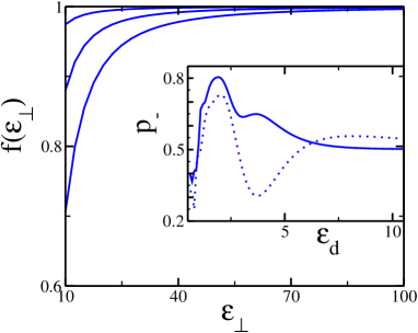
Figure 2: The main plot: the fidelity of the amplification versus $\epsilon_{\perp}$ for $n=4,\,8,\,12$ pulses from top to bottom. Inset: the probability $p_{-}$ versus $\epsilon_{d}$ at $\epsilon_{z}=4.0\omega_{0}$ (solid line) and $\epsilon_{z}=3.2\omega_{0}$ (dotted line). Here $\lambda_{0}=20\,\mathrm{GHz}$.

Ideal situations are assumed in the above discussions with well separated energy scales: $\epsilon_{\perp}\gg\omega_{0}$ during the amplification and $\epsilon_{z},\epsilon_{d},8n\alpha_{0}\lambda_{0}\gg\omega_{0}$ during the detection. In practice, the frequency of the resonator is around $100\,\mathrm{MHz}$; while the amplitudes of the pulses $\epsilon_{\perp}$, $\epsilon_{d}$ are upper bounded by the Josephson energy $E_{J0}$ of the charge qubit which is typically below $20\,\mathrm{GHz}$. The dynamics of the resonator may have important effects on our scheme. Below, we numerically simulate the dynamics of the amplification and detection with the above parameters and in the coordinate space of the resonator.

Let the wave function at time $t$ be $|\psi(t)\rangle=\sum_{s}\int dx|s\rangle|x\rangle\varphi_{s}(x,t)$ where $s$ is the state of the charge qubit and $\varphi_{s}(x,t)$ is the wave function of the resonator, with the initial state discussed above. We calculate the fidelity of the amplification process: $f(\epsilon_{\perp})=\left|\left\langle\psi_{id}\left(t\right)|\psi\left(t\right)\right\rangle\right|^{2}$, where $|\psi_{id}\rangle$ is the ideal wave function generated by the pulses in Eq. (2). In Fig.2, the fidelity is plotted versus the amplitude of the pulse $\epsilon_{\perp}$. It can be seen that at $\epsilon_{\perp}=10\omega_{0}$, the fidelity can be very low with $f=0.7$ after $n=12$ pulses; but the fidelity increases rapidly with increasing $\epsilon_{\perp}$. At $\epsilon_{\perp}=60\,\omega_{0}$, corresponding to $\epsilon_{\perp}=6\,\mathrm{GHz}$, the fidelity is $f>0.99$ after $n=12$ pulses. In the detection process, the dynamics of the resonator affects the probability $p_{-}$. We simulate the detection process at various static bias $\epsilon_{z}$ and with $\epsilon_{d}$ in the range of $0.5\,\omega_{0}\,-\,10.5\,\omega_{0}$. Here $8n\alpha_{0}\lambda_{0}\approx 1.9\,\omega_{0}$ after $n=12$ pulses. In the inset of Fig.2, $p_{-}$ is plotted versus $\epsilon_{d}$ at $\epsilon_{z}=3.2\,\omega_{0}$ and $\epsilon_{z}=4.0\,\omega_{0}$. When $\epsilon_{d}\gg 8n\alpha_{0}\lambda_{0}$, the charge qubit flips for both the states $|\pm 2n\alpha_{0}\rangle$ and $p_{-}\approx 0.5$. When $\epsilon_{d}\sim 8n\alpha_{0}\lambda_{0}$, the off resonance strongly affects $p_{-}$. For $\epsilon_{z}=4.0\,\omega_{0}$, a maxumum of $p_{-}$ appears at $\epsilon_{d}=1.9\omega_{0}$ with $p_{-}=0.80$, very different from the probability without the correlation. For $\epsilon_{z}=3.2\,\omega_{0}$, $p_{-}$ oscillates with $\epsilon_{d}$ due to the evolution of the resonator. This shows that the correlation between the resonator and the charge qubit can be detected even at high resonator frequency.

With a coupling of $20\,\mathrm{MHz}$Resonator_cooling , $n\geq 10$ flips are required to have $2n\alpha_{0}>1$, a duration around $50\,\mathrm{nsec}$. It is crucial to have a decoherence time longer than this duration to successfully generate the entanglement. During the amplification process, the charge qubit operates at the degenerate point where the charge noise, dominated by the low frequency charge fluctuations, causes a decoherence time of microsecondsoptimal_point . In the rotating frame of Eq. (1), this can be explained by a spectral shift: the noise spectrum in this frame is $S^{0}\left(\omega\pm E_{J0}/\hbar\right)$ with a shift of $E_{J0}$ from the noise spectrum in the lab frame $S^{0}\left(\omega\right)$. The low frequency noise is hence screened by the Josephson energy. The mechanical noise of the resonator can be described by the quality factor $Q$. At temperature $T=20\,\mathrm{mK}$ with $Q=10^{4}$, the dissipation rate is $k_{B}T/Q=50\,\mathrm{KHz}$. The decoherence rate is $\tau_{dec}^{-1}\approx(2n\alpha_{0})^{2}k_{B}T/Q$, which at $2n\alpha_{0}=5$ gives $\tau_{dec}^{-1}\sim 1\,\mathrm{MHz}$ and limits the amplification process. Meanwhile, in a situation where the phase coherence between the states $|\uparrow\rangle|-2n\alpha_{0}\rangle$ and $|\downarrow\rangle|2n\alpha_{0}\rangle$ is not required as in the spin detectionsingle_spin_detection , the amplitude of the generated coherent states can be bounded by the quality factor. Assume after $n_{s}$ flippings the amplification saturates. This means that starting from the coherent state $|-2n_{s}\alpha_{0}\rangle$ with the charge qubit at $|\uparrow\rangle$, after a time of $\pi/\omega_{0}$, the coherent state is $|2n_{s}\alpha_{0}\rangle$. The initial elastic energy is $\hbar\omega_{0}\alpha_{0}^{2}\left(2n_{s}+1\right)^{2}$, while the final elastic energy is $\hbar\omega_{0}\alpha_{0}^{2}\left(2n_{s}-1\right)^{2}$ with an energy loss of $\delta E=8n_{s}\hbar\omega_{0}\alpha_{0}^{2}$. The loss is caused by the dissipation: $\delta E=4\pi n_{s}^{2}\hbar\omega_{0}\alpha_{0}^{2}/Q$, from which the saturation limit: $n_{s}=2Q/\pi$ can be derived.

This scheme involves a generic model of one harmonic oscillator and one quantum two level system (spin) coupling via linear interaction $\hat{x}\sigma_{z}$, and hence can be generalized to other spin-oscillator systems. One example is the single spin detection by magnetic resonance force microscopy (MRFM)single_spin_detection where the spins near a surface interact with the magnetic particle attached to a cantilever and affect the vibration of the cantilever. By observing the frequency or amplitude of the vibration with optical interferometry, the distribution of the spins can be detected. In experiments, the resolution of MRFM has been improved towards the single spin levelsingle_spin_detection . In the conventional scheme, the cyclic adiabatic inversion (CAI) methodsingle_spin_detection is applied where the spins are driven by continuous microwave with periodic modulation of the phase of the microwave. Our scheme provides an alternative to this approach. By applying parametric pulses to flip the spins every half period of the cantilever, coherent states of the cantilever with large amplitude can be generated within a short time even at weak coupling. Using the same notations as that in Eq. (1) and assuming a total local spin of $m/2$ near the tip, after $n$ spin flips in Eq. (2), the coherent states are $|\pm 2nm\alpha_{0}\rangle$. This shows a resolution of $\delta\alpha/\delta m=2n\alpha_{0}$. When $2n\alpha_{0}\gg 1$ and $n_{s}\geq n$, single spin resolution can be achieved. This requires $Q>\pi/4\alpha_{0}$ of the cantilever.

We studied a scheme of generating and detecting Schrödinger cat state in the coupled resonator and SCPB system. Compared with previous worksresonator_SCPB1 ; resonator_SCPB2 , large amplitude coherent states can be obtained at much smaller coupling than the energy of the resonator. The scheme provides a practical way of investigating the quantum properties of the nanomechanical resonators.

Acknowledgments: We thank I. Wilson-Rae, A. Shnirman and P. Zoller for helpful discussions. This work is supported by the Austrian Science Foundation, the CFN of the DFG, the Institute for Quantum Information, and the EU IST Project SQUBIT.

References

(1) R.G. Knobel and A.N. Cleland, Nature 424,
291 (2003); M.D. LaHaye et al., Science 304, 74 (2004).
(2) A.N. Cleland and M.L. Roukes, Nature 392,
160 (1998); H.G. Craighead, Science 290, 1532 (2000); X. Ming
et al., Nature 421, 496 (2003).
(3)
V.B. Braginsky and F.Y. Khalili, Quantum Measurement, Cambridge
Univ. Press, Cambridge (1992).
(4)
W.J. Munro et al, Phys. Rev. A 66, 023819 (2002).
(5) A.N. Cleland and M.R. Geller, Phys. Rev. Lett.
93, 070501 (2004).
(6) A. D. Armour, M. P. Blencowe, and K. C.
Schwab, Phys. Rev. Lett. 88, 148301 (2002).
(7) E.K. Irish and K. Schwab, Phys. Rev. B
68, 155311 (2003).
(8) A. Hopkins et al., Phys. Rev. B. 68, 235328 (2003).
(9)
I. Wilson-Rae, P. Zoller and A. Imamolu,
Phys. Rev. Lett. 92, 075507 (2004).
(10) I. Martin et al.,
Phys. Rev. B 69, 125339 (2004).
(11) D.J. Wineland et al., J. Res. Natl.
Inst. Stand. Technol. 103, 259 (1998).
(12) Y. Makhlin, G. Schön, and A. Shnirman,
Rev. Mod. Phys. 73, 357 (2001).
(13)
S. Lloyd and S.L. Braunstein, Phys. Rev. Lett. 82, 1784 (1999).
(14) D. Rugar et al., Nature
430, 329 (2004); J.A. Sidles et al., Rev. Mod. Phys.
67, 249 (1995).
(15) D. Vion et al., Science 296, 886
(2002).
(16)
B. Kraus et al., Phys. Rev. A 67, 042314 (2003).