A differential method for bounding the ground state energy

Abstract

For a wide class of Hamiltonians, a novel method to obtain lower and upper bounds for the lowest energy is presented. Unlike perturbative or variational techniques, this method does not involve the computation of any integral (a normalisation factor or a matrix element). It just requires the determination of the absolute minimum and maximum in the whole configuration space of the local energy associated with a normalisable trial function (the calculation of the norm is not needed). After a general introduction, the method is applied to three non-integrable systems: the asymmetric annular billiard, the many-body spinless Coulombian problem, the hydrogen atom in a constant and uniform magnetic field. Being more sensitive than the variational methods to any local perturbation of the trial function, this method can used to systematically improve the energy bounds with a local skilled analysis; an algorithm relying on this method can therefore be constructed and an explicit example for a one-dimensional problem is given.

PACS : 03.65.Db, 05.45.Mt, 02.30.Tb, 02.60.Gf.

1 Introduction

In a large variety of interesting physical problems, finding the discrete spectrum of an operator can be done with approximate methods only. Moreover, in most cases, it is a rather difficult task to estimate errors. Perturbative techniques often lead to non-convergent series and an evaluation of the discrepancies with the exact result is usually beyond their scope. For semibounded operators, variational methods naturally provide upper bounds for the lowest eigenvalue and require much more work for providing a lower bound with Temple-like methods [Reed/Simon78a, XIII.2]. Another source of difficulties when dealing with perturbative and/or variational techniques, is that they both involve the calculation of integrals on the configuration space $\mathcal{Q}$: the norm of the wavefunctions and some matrix elements of operators. This reflects the fact that the discrete spectrum of a differential operator encapsulates some global information on $\mathcal{Q}$ within the boundary conditions imposed on the normalisable wavefunctions. In this article, I want to propose an approximate method that will overcome these two obstacles: it can rigorously provide both lower and upper bounds without any kind of integration. Like the variational techniques, it will involve a (set of) trial normalisable function(s) with the appropriate boundary conditions and will concern in practice the lowest eigenvalue only. The bounds are given by the absolute extrema of a function defined on $\mathcal{Q}$ (the so-called local energy). In a sense, this method allows to stay as local as possible in the configuration space $\mathcal{Q}$: in order to improve the bounds, a local analysis near the extrema (or near the possible singular points) of the local energy is sufficient and necessary. This paper is organised as follows. In section 2, I give the proof of the inequalities that will be the starting point of the differential method. A comparison with what already exists in the litterature follows and the guidelines of the method are presented. Sections 3, 4 and 5 show how the method can be applied to three non-integrable quantum systems. Before the concluding remarks, in section 6, I explicitely show on the quartic oscillator how the sensitivity of the differential method to local perturbations of the trial functions can be exploited to systematically improve the bounds of the ground state energy with an elementary algorithm.

2 Bounding the ground state energy with the local energy

Let us start with a quantum system whose Hamiltonian $\hat{H}$ acts on the Hilbert space of functions defined on a configuration space $\mathcal{Q}$. Let us suppose that $\hat{H}$ has an eigenstate $|\Phi_{0}\rangle$ associated with an element $E_{0}$ of the discrete spectrum. For any state $|\varphi\rangle$, the hermiticity of $\hat{H}$ implies the identity $\langle\Phi_{0}|(\hat{H}-E_{0})|\varphi\rangle=0$. If we choose $|\varphi\rangle$ such that its configuration space representation $\varphi(q)$ is a smooth real normalisable wavefunction, we obtain:

$$\int_{\mathcal{Q}}\Phi^{*}_{0}(q)(H-E_{0})\varphi(q)\,dq=0\;.$$ (1)

The crucial positivity hypothesis is to assume that we can choose one eigenstate such that its eigenfunction $\Phi_{0}$ remains real and positive or zero in the whole $\mathcal{Q}$. This generally applies to the ground state for which it has been shown in many cases that it is strictly positive in the interior of $\mathcal{Q}$ [Reed/Simon78a, XIII.12]. Then, the real part of (1) involves an integrand that is a smooth, real function constructed from the real part $H_{\!R}$ of the differential operator $H$. Then there exists a $q$ in $\mathcal{Q}$ such that $\Phi_{0}(q)(H_{\!R}-E_{0})\varphi(q)$ changes its sign. Therefore,

$$\exists\,q\in\mathcal{Q}\quad\text{such that}\quad(H_{\!R}-E_{0})\varphi(q)=0\;.$$ (2)

Let us now introduce a function on $\mathcal{Q}$ that is known as the local energy

$$E_{\mathrm{loc}}^{[\varphi]}(q)\ \stackrel{{\scriptstyle\mathrm{def}}}{{=}}\ \frac{H_{\!R}\,\varphi(q)}{\varphi(q)}\;.$$ (3)

From condition (2), we immediately obtain that for all smooth real and normalisable state $\varphi$,

$$\inf_{\mathcal{Q}}\big{(}E_{\mathrm{loc}}^{[\varphi]}(q)\big{)}\leqslant\ E_{0}\ \leqslant\sup_{\mathcal{Q}}\big{(}E_{\mathrm{loc}}^{[\varphi]}(q)\big{)}\;.$$ (4)

Surprisingly, these two inequalities are sparsely known in the literature [Barnsley78a, Baumgartner79a, Thirring79b, Crandall/Reno82a, Schmutz85a] and always under some more restricted conditions (the upper bound is often missing).

The original proof presented here links the inequalities to the non-negativity of the ground state without referring to the detailed structure of the Hamiltonian. In particular, it does not require for the Hamiltonian to have the purely quadratic form

$$\hat{H}=\sum_{i,j}a_{i,j}\hat{p}_{i}\hat{p}_{j}+V(\hat{q})$$ (5)

where $a$ is a definite positive real matrix and $V$ a well-behaved potential. Inequalities (4) still apply (with the appropriate definition (3) of the local energy) in the presence of a singular potential, when there is a magnetic field and for an infinite number of freedoms (like in the non-relativistic quantum field describing a BEC condensate). Besides, it is not required for $\varphi$ to be nonvanishing. It simply says that where $\varphi$ vanishes faster than $H_{\!R}\,\varphi$, one or both of the bounds can be infinite and therefore useless.

The first form of inequalities (4) (with its two bounds) is due to Barta [Barta37a] and was derived for the fundamental vibration mode of an elastic membrane. Though Barta writes that his method will be generalised in subsequent publications, I was not able to find any extensions of his original work before an article of Duffin [Duffin47a] where a Schrödinger operator of the form $H=-\Delta+V$ is considered. Duffin shows that the Dirichlet boundary conditions imposed on the trial function $\varphi$ can be relaxed but he loses the upper bound. One obtains the equalities in (4) for a flat local energy i.e. for $\varphi=\Phi_{0}$; hence we will try to work with a $\varphi$ that mimics the exact ground state best. Therefore, generalising the Barta inequalities by increasing the size of the functional space of $\varphi$’s can be irrelevant. One should instead keep working with a restricted set of trial functions that respects some a priori known properties of $\Phi_{0}$, such as its boundary conditions, its symmetries and its positivity.

More precisely, we will explain in the last part of this paper that, once a $\varphi$ that bounds the local energy is found, it is expected that there is only a finite number of independent directions in the functional space along which the bounds can be improved. In the following we will actually deal with a finite dimensional submanifold of trial functions $\varphi_{\lambda}$ where $\lambda$ stands for a small number of control parameters varying in a control space $\mathcal{C}$. Accordingly, the strategy is clear: for, say, obtaining an optimized lower bound we will try to find $\sup_{\lambda\in\mathcal{C}}\left(\inf_{q\in\mathcal{Q}}\big{(}E_{\mathrm{loc}}(\lambda;q)\big{)}\right)$ where $E_{\mathrm{loc}}(\lambda;q)$ stands for $E_{\mathrm{loc}}^{[\varphi_{\lambda}]}(q)$. As long as the extremal values of $q\mapsto E_{\mathrm{loc}}(\lambda;q)$ can be followed smoothly with $\lambda$ (in particular the Morse points are generically stable), the problem is reduced to local differential calculations in $\mathcal{C}\times\mathcal{Q}$ in the neighborhood of the critical points: adding to a trial function an infinitesimal perturbation that is localized far away from the extremal point does not affect the energy bounds. One recovers the global sensitivity of the eigenvalue problem because the critical points of the local energy generically bifurcate for finite variations of $\lambda$ [Poston/Stewart78a, Demazure00a] and can jump to other distant points when a degeneracy occurs [Arnold84a, chap. 10, especially fig. 50].

In mathematical physics literature, Barta’s inequalities are always considered within the context of the billiards systems (Laplacian spectra on a Riemannian manifold), even in the most recent papers (for instance [Pacelli/Montenegro04a]). As far as I could search, the most advanced extension to other physical problems has been made (tentatively) by Barnsley [Barnsley78a] but, for the same reasons as Duffin’s [Duffin47a], he systematically loses the upper bound. Besides, he acknowledges he is unable to produce any non-trivial bound for the Helium atom.

One can easily understand Barnsley’s failure: With variational methods, a very rough estimation of the exact ground state wavefunction can lead to a reasonably good agreement for $E_{0}$ while a simple local perturbation of the exact wave function can even make the local energy unbounded. Therefore, at first sight, one could see the sensitivity of the local energy as a major drawback of the method: variational methods are more robust to local perturbations of the trial function. But this argument can be reversed : compared to the rigidity of the variational methods, the differential method offers the possibility to improve the estimations at low cost provided we are able to implement a skilled strategy (eliminating the singularities, controlling the behavior at infinity with jwkb techniques, increasing the absolute minimums, etc.). In the following, I explicitly show in many non-trivial cases, that once we have this strategy in mind, we can obtain interesting results for complex systems. For instance, not only we can improve Barnsley’s trivial bound for the ground state energy of the Helium atom, but it will be shown in section 4 how this result generalizes to any number of Coulombian particles. The calculations can be made analytically with a surprising simplicity.

As far as the upper bound is concerned, the variational method leads a priori to a better approximation than the differential method since, for any normalised function $\phi$,

$$\int_{\mathcal{Q}}\varphi^{*}(q)H\varphi(q)\,dq=\int_{\mathcal{Q}}|\varphi(q)|^{2}E_{\mathrm{loc}}^{[\varphi]}(q)\,dq\leqslant\sup_{\mathcal{Q}}\big{(}E_{\mathrm{loc}}^{[\varphi]}(q)\big{)}\;.$$ (6)

Nevertheless, being free of any integration, the absolute maximum of the local energy is a quantity that is more easily accessible to analytical or numerical computations than the average value of $H$.

3 Application to billiards; the example of the 2d-annular billiard

As a first illustration of the differential method, let us consider the problem of finding the lowest eigenvalue of $H=-\Delta/2$ in a connected finite region $\mathcal{Q}$ with the Dirichlet boundary conditions imposed on $\mathcal{B}\stackrel{{\scriptstyle\mbox{\rm\tiny def}}}{{=}}\partial\mathcal{Q}$. Suppose that the boundary $\mathcal{B}$ is given by an implicit smooth scalar equation of the form $b(q)=0$ while the interior of $\mathcal{Q}$ is defined to be the set of points $q$ such that $b(q)<0$. Then, trial functions can be taken of the form $\varphi=fb$ for any arbitrary smooth function $f$ that does not vanish inside $\mathcal{Q}$. The only possible singular points of $q\mapsto E_{\mathrm{loc}}^{[\varphi]}(q)$ are located on $\mathcal{B}$ and can be removed if $f$ is chosen with an appropriate behaviour in the neighborhood of $\mathcal{B}$. Imposing this behaviour for $f$ is a priori a simpler task than solving the eigenvalue problem on the global $\mathcal{Q}$: one dimension has been spared since we have to deal with some local properties of $f$ near $\mathcal{B}$. For instance, by generalizing Barta’s trick [Barta37a], one can easily check by a simple equation counting that when $\mathcal{Q}$ is algebraic i.e. when $b$ is a polynomial, provided that we choose $f$ to be a polynomial of sufficiently high degree $n$ whose zeros are outside $\mathcal{Q}$, we can find a polynomial $g$ of degree $n-2$ such that $\Delta(fb)=gb$. Therefore $E_{\mathrm{loc}}^{[\varphi]}=-g/(2f)$ is bounded and finite upper and lower bounds of $E_{0}$ can be found. Let us apply this method to the asymmetric annular billiard that is an elegant paradigmatic model in quantum chaos [Bohigas+93a]. $\mathcal{B}$ is made of two circles of radius $1$ and $r<1$ whose centers are distant by $\delta<1-r$. $\mathcal{Q}$ is the 2d-domain in between the circles. The simplest choice of trial function is to take $\varphi(x,y)=b(x,y)=[x^{2}+y^{2}-r^{2}][(x-\delta)^{2}+y^{2}-1]$. One can check analytically that the lower bound of $E_{\mathrm{loc}}^{[\varphi]}$ is

$$\inf_{\mathcal{Q}}\left(\frac{-\Delta\varphi}{2\varphi}\right)=\sup_{\mathcal{Q}}\left(\frac{8[(x-\delta/2)^{2}+y^{2}-(1+r^{2})/4]}{[x^{2}+y^{2}-r^{2}][(x-\delta)^{2}+y^{2}-1]}\right).$$ (7)

For $r=3/4$ and $\delta=0.1$, a simple numerical computation shows that (7) is finite and obtained at $(x,y)\simeq(0.86,0)$ and leads to $E_{0}\geqslant 28.390$ to be compared with the exact result $E_{0}\simeq 42.94$. As one could have expected with the rough trial function chosen above, the estimation is not very precise but the calculations required here to get this result are much simpler than the ones involved in a variational method (that provides the complementary upper bound $55.32$ with the same test function) or by the exact numerical resolution that requires to find the smallest root of an infinite determinant made of Bessel functions.

4 The many-body Coulombian problem

The next examples, presented in this section and in the following, will illustrate that the first strategy for obtaining finite bounds is to get rid of the singularities that may appear in the local energy. When $\mathcal{Q}$ is not bounded, one must have a control over the behaviour of the trial functions as $q$ goes to infinity. For a multidimensional, non separable, Schrödinger Hamiltonian, a jwkb-like asymptotic expression is generally not available [Maslov/Fedoriuk81a, Introduction]. Nevertheless, the differential method is less demanding than the semiclassical approximations: we will ask that the local energy be bounded at infinity but we will not require it to tend to the same limit in all directions. As already shown in the annular billiard problem, for the sake of simplicity one could start with a less ambitious program and try to obtain just one nontrivial inequality in (4).

The second example is to consider a system of $N$ non-relativistic, spinless, charged particles living in a $D$-dimensional infinite space. Their kinetic energy is given by $\sum_{i=0\dots N-1}\hat{p}_{i}^{2}/(2m_{i})$ and they interact with each other via a two-body Coulombian interaction $e_{i}e_{j}/\hat{r}_{ij}$. We will assume that the masses $m_{i}$ and the charges $e_{i}$ allow the existence of a bound state. Once the free motion of the center of mass is discarded, we are led to a $D(N-1)$-dimensional configuration space that can be described by the relative positions $q=\{\mathbf{r}_{0,i}\}_{i=1\dots N-1}$ with respect to one distinguished particle. The Hamiltonian is given by

$$\hat{H}=\sum_{i=1}^{N-1}\frac{1}{2m_{0,i}}\hat{\mathbf{p}}_{i}^{2}+\frac{1}{2m_{0}}\sum_{\begin{subarray}{c}i,j=1\\ i\neq j\end{subarray}}^{N-1}\hat{\mathbf{p}}_{i}.\hat{\mathbf{p}}_{j}+\frac{1}{2}\sum_{\begin{subarray}{c}i,j=0\\ i\neq j\end{subarray}}^{N-1}\frac{e_{i}e_{j}}{\hat{r}_{i,j}}\;.$$ (8)

The notation $m_{i,j}$ stands for the reduced mass $m_{i}m_{j}/(m_{i}+m_{j})$. For $D\geqslant 2$, one can eliminate the Coulombian simple poles $r_{i,j}=||\mathbf{r}_{0,i}-\mathbf{r}_{0,j}||=0$ in the local energy by choosing the trial function as follows:

$$\varphi(q)=\exp\Big{(}-\frac{1}{2}\sum_{\begin{subarray}{c}i,j=0\\ i\neq j\end{subarray}}^{N-1}\lambda_{i,j}r_{i,j}\Big{)}$$ (9)

with $\lambda_{i,j}=-2m_{i,j}e_{i}e_{j}/(D-1)$. When this choice does not provide a normalisable function, it should be understood that the exponent is just the first order of a Taylor expansion near $r_{i,j}=0$. Whenever (9) is actually square integrable on $\mathcal{Q}$, the local energy reads

$$E_{\mathrm{loc}}^{[\varphi]}=-\sum_{\begin{subarray}{c}i,j=0\\ i<j\end{subarray}}^{N-1}\frac{\lambda_{i,j}^{2}}{2m_{i,j}}-\sum_{\widehat{j,i,k}}\frac{\lambda_{i,j}\lambda_{i,k}}{m_{i}}\cos(\widehat{j,i,k}).$$ (10)

The last sum involves all the angles $\widehat{j,i,k}$ that can be formed with all the triangles made of three distincts particles. This expression treats all the particles on an equal footing and it is clear that the local energy is bounded everywhere. Bounding simultaneously all the $\cos(\widehat{j,i,k})$ by $\pm 1$ can be a rather crude approximation. One should instead take into account the correlation between the angles. For instance, when $D=3$, as soon as $N\geqslant 3$, their number ($N(N-1)(N-2)/2$) exceeds the number of independent variables minus three Euler angles and a dilatation factor $3(N-1)-3-1$). For $N=2$, we recover the exact ground state since the last sum is absent and the local energy is constant. For a helium like atom ($D=3$, $N=3$) of charge $(Z-2)e$ with the nucleus considered as infinitely massive compared to the electron mass, only two angular terms survive and we get (in atomic units) $E_{\mathrm{loc}}=-Z^{2}-1/4+Z(\cos\theta_{1}+\cos\theta_{2})/2$. The two angles are taken at the vertices made by the two electrons: the sum of their cosines is bound from below by 0 and from above by 2 (diametrically opposed electrons). The lower bound of the local energy is $-Z^{2}-1/4$; this is not an interesting piece of information since we know that $E_{0}$ is larger than the energy $-Z^{2}$ obtained by neglecting the strictly positive repulsion of the electrons. On the other hand the bound $E_{0}\leqslant-(Z-1/2)^{2}$ provides a simple, analytical, non-trivial result.

5 The hydrogen atom in a magnetic field

The third application of the differential method to a non-integrable system will concern the hydrogen atom in a constant and uniform magnetic field $B\vec{u}_{z}$. While the positivity of the ground state wavefunction was guaranteed by the so-called Krein-Rutman theorem in all the previous examples (applicable for any Hamiltonian of the form (5), see for instance [Reed/Simon78a, XIII.12]), it is not valid any longer for an arbitrary potential when a magnetic field is present [Helffer+99a]. Nevertheless, for the hydrogen atom, the attractive interaction between the nucleus and the electron keeps the orbital momentum $L_{z}$ of the ground state at zero for any arbitrary value of $B$ [Avron+77a] and the Krein-Rutman theorem applies when restricted to the $L_{z}=0$ subspace. In order to preserve the symmetry of the ground state, the trial function will be chosen to be strictly positive and even with respect to $z$; hence we can work in the half space where $z\geqslant 0$. With a vanishing paramagnetic term, $\varphi$ depends on the coordinates $q=(\rho,r)$ only (see FIG. 1). In atomic units, the local energy is given by $E_{\mathrm{loc}}^{[\varphi]}=V-\Delta\,\varphi/(2\varphi)$ where the effective potential is $V(\rho,r)=B^{2}\rho^{2}/8-1/r$. In order to eliminate the Coulomb singularity, one must impose some local conditions on the logarithmic derivatives of $\varphi$. More precisely, with $S\stackrel{{\scriptstyle\mbox{\rm\tiny def}}}{{=}}\ln\varphi$, we must have $\partial_{r}S(0,0)=-1$ and $\partial_{\rho}S(0,r)=0$ for all $r\geqslant 0$. Assuming that $S$ is smooth enough near $\rho=0$, it takes the general form $S(\rho,r)=-r+r^{2}l(r)+\rho^{2}h(\rho,r)$ where $l$ and $h$ are two smooth functions. Choosing $l\equiv 0$ and $h\equiv-B/4$ [resp. $h\equiv 0$] will bound from above [resp. below] the local energy: $-1/2\leqslant E_{0}\leqslant-1/2+B/2$. Like in the previous example the lower bound is useless since it can be guessed from the very beginning. The real challenge here is to improve the lower bound without introducing a divergence as $r\to\infty$ in any direction characterized by $\alpha$. After a detailed examination of the possible balance between the asymptotic behaviour of $l$ and $h$ as $r\to\infty$, a trial function can be constructed in order to improve the trivial lower bound for $B$ large enough. Namely if we take $S=-r-B\rho^{2}/4+\rho^{2}(r-\sqrt{r^{2}-\rho^{2}})/(\rho^{2}+5r/\sqrt{B})$ we improve the trivial lower bound for $B\gtrsim 2.3$ (see FIG.1). Note that for very large $B$ we recover a wavefunction that mimics a Landau state.

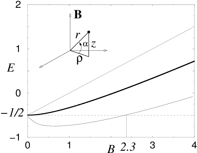
Figure 1: Upper and lower bounds of the ground state energy (thick line) for the hydrogen in a Zeeman configuration.

6 A local algorithm for improving the bounds ; application to the quartic oscillator

Assume now that $\varphi_{0}=\exp(S_{0})$ bounds the local energy. Is there any systematic strategy to improve the bounds and, one day, compete with the very high precision of the secular variational and perturbative methods or numerical diagonalisation of truncated matrices ? Of course one can always combine these four approaches but let us look, for the moment, how the local character of the differential method can be exploited further. Suppose that $q_{0}$ is a point where $q\mapsto E_{\mathrm{loc}}^{[\varphi_{0}]}(q)$ reaches its lowest non-degenerate value. Among all the possible infinitesimal perturbations of $S_{0}$, only those that are localised in the neighbourhood of $q_{0}$ are relevant since adding a perturbation far away from $q_{0}$ will not affect the absolute minimum. The appropriate framework for local studies in an infinite functional space is bifurcation theory. Since the local energy, the determination of the critical points and their stability involve a finite number of derivatives, we expect that the number of relevant control parameters $\lambda$ remains finite for low-dimension configuration space very much like the central result of catastrophe theory [Poston/Stewart78a, Demazure00a]. We will leave this quantitative study for future investigations. For the moment, let us keep the discussion at a qualitative level only with a 1d Hamiltonian of the form $H=-\Delta/2+V$ and take $S=S_{0}+\delta S$ with a Gaussian perturbation $\delta S(q)=s\exp(-(q-a)^{2}/\sigma^{2})$ controlled by three parameters $\lambda=(s,a,\sigma)$. The specific choice of the form of $\delta S$ is not important here ; only a finite number of pointwise derivatives will matter for locally improving the bounds as long as $\delta S$ does not change the normalisability of the trial function. The choice of a gaussian is particularly simple: it will modify the local energy in a neighbourhood of $a$ whose size is governed by $\sigma$ and by the magnitude $s$. This perturbation is qualitatively reproduced in FIG.2. The value of $E_{\mathrm{loc}}$ at $q=a$ is increased (resp. decreased) for a small but finite positive (resp. negative) $s$. We can apply this procedure near the absolute minimum (resp. maximum) of $E_{\mathrm{loc}}$ and repeat it for the possible absolute extrema that may have emerged during the previous step. We get an iteration sequence that may systematically improve the bounds. Still, this algorithm is slowed down because if we try to “lift up the dress” too much, a “prudish censor” lowers it on the both sides of $q=a$ (this phenomenon is not specific to 1d).

Figure 2: Increasing $E_{\mathrm{loc}}^{[\varphi_{0}]}$ (dashed line) with one local perturbation is limited. When adding to $\ln(\varphi_{0})$, say, a gaussian perturbation localised near an isolated minimum of the local energy, we can increase the value of the absolute minimum by a finite amount (solid line in the left figure). But if the magnitude of the Gaussian is increased too much, the minimums created by passing through a bifurcation can decrease below the original minimum (solid line in the right figure).

To be more precise, consider a quartic potential given by $V(q)=r^{2}q^{2}(q^{2}+\eta\,\delta^{2})/2$ where $\eta=\pm 1$. In order to bound the local energy as $|q|\to\infty$, we can use a jwkb-like expansion for $S_{0}$. If we want a uniformly smooth expression, we can take

$$\begin{split}S_{0}(q)=-\frac{1}{3}r(q^{2}+\delta^{2})^{3/2}+\frac{1}{2}r\delta^{2}(1-\eta)(q^{2}+\delta^{2})^{1/2}\\ -\frac{1}{2}\ln(q^{2}+\delta^{2})-\frac{1}{2}r\delta^{4}(q^{2}+\delta^{2})^{-1/2}\;.\end{split}$$ (11)

Figure 3: Adding $n$ Gaussians to $S_{0}$ allows to increase the minimum of the local energy when constructing the sequence $E_{\mathrm{loc}}^{(n)}$. For each iteration, only one scalar parameter is optimized (the amplitude of the gaussian being added).

The last term is chosen to improve the trivial lower bound given by the minimum of $V$. For the arbitrary choice $r=1/\sqrt{2}$, $\eta=-1$ and $\delta^{2}=8$, FIG. 3 shows how the lower bound can be improved from $-3.27$ up to $-2.74$ (the exact result is -2.66) when adding to $S_{0}$ enough Gaussians that are equi-spaced by $.5$ with a fixed $\sigma=1$. Only their magnitude $s$ are numerically optimized here, one after another. One can see a second advantage of the differential method when numerically implemented: not only no integral is required but also, provided we keep under control the instabilities that are illustrated in FIG. 2, the optimization algorithm concerns a small number of parameters at each step (just one in the example given in FIG. 3) to be compared with the large number of parameters to be optimized at one go in the final step of the variationnal method.

7 Conclusion

The differential method appears to be new kind of general theoretical tool for obtaining rigourous information on a ground state energy. Its local character makes it quite different from the traditional ones (to put it succintly, the variational, the perturbation and the numerical diagonalization techniques). In this paper, I have given some qualitative and quantitative arguments to show how simple and efficient it can be. However, I should insist that even in the cases where the variational or perturbative techniques can be applied, the aim of the paper is not to seek for performance: for the moment the differential method is too young to compete by itself with the traditionnal methods. One short term possibility is to calculate the extrema of the local energy constructed with the trial function given by the other methods. The idea of locally modifying the local energy or any local function of the same type — for instance, those currently used in Monte-Carlo methods — may be fruitful as well [Caffarel04a]. Actually, in order to convince the reader that the method is indeed applicable in a wide field of physics and furnishes some reasonable results, I had to compare them with some more precise ones and therefore I dealt with situations where the exact ground state energy was already known with the help of other methods. The algorithm that is presented in section 6 is chosen to prove how the local sensitivity of the local energy can be exploited to systematically improve the bounds. The feasibility is in itself not obvious and is worth to be demonstrated even in the simplest cases.

This work could not have been started without Hector Giacomini’s brilliant intuition that some relevant information on $E_{0}$ could be extracted from (2). I am very indebted to Dominique Delande and Benoît Grémaud for sharing their penetrating thoughts, their skilled numerical calculations in Coulombian problems and, not least, their kindful hospitality at the Laboratoire Kastler Brossel.

References

- [1] \harvarditem[Arnold]Arnold1984Arnold84a Arnold V.I. (1984): Catastrophe Theory. New York: Springer-Verlag.
- [2] \harvarditem[Avron, Herbst & Simon]Avron, Herbst & Simon1977Avron+77a Avron J., Herbst I. & Simon B. (1977): “The Zeeman effect revisited”, Phys. Lett. A, 62, pp. 214–216.
- [3] \harvarditem[Barnsley]Barnsley1978Barnsley78a Barnsley M. (1978): “Lower bounds for quantum mechanical energy levels”, J. Phys. A, 11(1), pp. 55–68.
- [4] \harvarditem[Barta]Barta1937Barta37a Barta J. (1937): “Sur la vibration fondamentale d’une membrane”, C. R. Acad. Sci. Paris, 204(7), pp. 472–473, (in french).
- [5] \harvarditem[Baumgartner]Baumgartner1979Baumgartner79a Baumgartner B. (1979): “A class of lower bounds for Hamiltonian operators”, J. Phys. A, 12(4), pp. 459–467.
- [6] \harvarditem[Bessa & Montenegro]Bessa & Montenegro2004Pacelli/Montenegro04a Bessa G.P. & Montenegro J.F. (2004): “An Extension of Barta’s Theorem and Geometric Applications”, eprint arXiv:math/0308099.
- [7] \harvarditem[Bohigas, Boosé, Egydio de Carvalho & Marvulle]Bohigas, Boosé, Egydio de Carvalho & Marvulle1993Bohigas+93a Bohigas O., Boosé D., Egydio de Carvalho R. & Marvulle V. (1993): “Quantum tunneling and chaotic dynamics”, Nuclear Phys. A, 560, pp. 197–210.
- [8] \harvarditem[Caffarel]Caffarel2004Caffarel04a Caffarel M. (2004): private communication.
- [9] \harvarditem[Crandall & Reno]Crandall & Reno1982Crandall/Reno82a Crandall R.E. & Reno M.H. (1982): “Ground state energy bounds for potentials ”, J. Math. Phys., 23(1), pp. 64–70, erratum[J. Math. Phys. 23, 1737 (1982)].
- [10] \harvarditem[Demazure]Demazure2000Demazure00a Demazure M. (2000): Bifurcations and Catastrophes, Universitext. Springer.
- [11] \harvarditem[Duffin]Duffin1947Duffin47a Duffin R.J. (1947): “Lower bounds for eigenvalues”, Phys. Rev., 71, pp. 827–828.
- [12] \harvarditem[Helffer, Hoffmann-Ostenhof & Owen]Helffer, Hoffmann-Ostenhof & Owen1999Helffer+99a Helffer B., Hoffmann-Ostenhof T. & Owen M. (1999): “Nodal sets for groundstates of the SchrÖdinger with zero magnetic fields in a non simply connected domain”, Comm. Math. Phys., 202, pp. 629–649.
- [13] \harvarditem[Maslov & Fedoriuk]Maslov & Fedoriuk1981Maslov/Fedoriuk81a Maslov V.P. & Fedoriuk M.V. (1981): Semi-Classical Approximation in Quantum Mechanics, vol. 7 of Mathematical physics and applied mathematics. Dordrecht: D. Reidel publishing company.
- [14] \harvarditem[Poston & Stewart]Poston & Stewart1978Poston/Stewart78a Poston T. & Stewart I. (1978): Catastrophe Theory and its Applications. London: Pitman.
- [15] \harvarditem[Reed & Simon]Reed & Simon1978Reed/Simon78a Reed M. & Simon B. (1978): Analysis of operators, vol. 4 of Methods of modern mathematical physics. New York: Academic Press.
- [16] \harvarditem[Schmutz]Schmutz1985Schmutz85a Schmutz M. (1985): “The factorization method and ground state energy bounds”, Phys. Lett. A, 108(4), pp. 195–196.
- [17] \harvarditem[Thirring]Thirring1979Thirring79b Thirring W. (1979): Quantum mechanics of atoms and molecules, vol. 3 of A course in mathematical physics. New York: Springer-Verlag.
- [18]