Quantum limits of super-resolution in reconstruction of optical objects

Abstract

We investigate analytically and numerically the role of quantum fluctuations in reconstruction of optical objects from diffraction-limited images. Taking as example of an input object two closely spaced Gaussian peaks we demonstrate that one can improve the resolution in the reconstructed object over the classical Rayleigh limit. We show that the ultimate quantum limit of resolution in such reconstruction procedure is determined not by diffraction but by the signal-to-noise ratio in the input object. We formulate a quantitative measure of super-resolution in terms of the optical point-spread function of the system.

I Introduction

Quantum imaging is a new branch of quantum optics that investigates the ultimate performances of optical imaging allowed by the laws of quantum mechanics Kolobov99 ; Lugiato02 . One of the pertinent questions of quantum imaging is about the quantum limits of the optical resolution. The classical resolution limit was established by Abbe and Rayleigh at the end of the nineteen century and is very well known nowadays. The Rayleigh resolution criterion states that the resolution in an optical system is limited by diffraction on its optical elements due to the wave nature of the light. According to this criterion, two closely spaced points at the input of the optical system cannot be resolved if the distance between them is smaller than $\lambda/{\rm NA}$ where $\lambda$ is the wavelength of the light and ${\rm NA}$ - the numerical aperture of the optical system.

This classical resolution limit is based on the presumed resolving capabilities of the human eye and is not a fundamental limit like, for example, the Heisenberg uncertainty relation. Nowadays using modern CCD cameras for detection of optical images with subsequent electronic processing one can often improve the resolution beyond the classical diffraction limit. For example, while the Rayleigh criterion puts the resolution limit of about 0.2 $\mu$m for an optical microscope, by processing microscopic images one can achieve a precision of about 1nm Kamimura87 . Even more spectacular results has been obtained recently for detection of a small displacement of a laser beam Treps03 . Using ”spatially squeezed” laser beam the authors of Treps03 have succeeded to measure a transverse displacement of 1.6 Angstrom of a laser beam with wavelength $\lambda=1064$ nm.

These two experiments are particular examples of the so-called super-resolution techniques that aim to improve the optical resolution beyond the classical diffraction limit. Super-resolution is possible when one has some a priori information about the object. For example, in practice one usually deals with objects of finite size. In this case one can obtain super-resolution because the spatial Fourier spectrum of such objects, produced in the focal plane of a lens where the system pupil is located, is an analytical function. Thus, measuring a part of the Fourier spectrum, transmitted by the system pupil, one can in principle reconstruct the rest of the spectrum via the analytical continuation and, therefore, obtain an infinite resolution. However, the procedure of such an analytical continuation is extremely sensitive to different kind of noises present in the optical system. Recently it was shown Kolobov00 that the ultimate limit of resolution in diffraction-limited imaging is determined not by diffraction but by the quantum fluctuations of light within the object area and the vacuum fluctuations outside it. These quantum fluctuations set up the standard quantum limit of resolution which can be by the orders of magnitude smaller than the diffraction limit. Moreover, one can further improve the resolution beyond the standard quantum limit using multimode squeezed light. An optical scheme of such a super-resolution microscopy with squeezed light was proposed in Ref. Sokolov04 .

In this paper we numerically simulate the role of quantum fluctuations in reconstruction of optical objects from the diffraction-limited images. We take as example of an input object two Gaussian peaks placed so close to each other that in the output image they cannot be resolved according to the Rayleigh criterion. We assume that one can measure the spatial Fourier components of the input object in the focal plane of the imaging lens within the pupil area. This kind of measurement corresponds to the super-resolving Fourier-microscopy Scotto03 since instead of observing the image one observes its spatial Fourier spectrum. We formulate the quantum theory of this microscopy in terms of the prolate spheroidal functions very similar to the theory developed in Ref. Kolobov00 . Using this quantum theory, we simulate numerically the reconstructed objects and investigate the role of quantum fluctuations on their resolution.

Our numerical simulations allow us to confirm that when quantum fluctuations are not taken into account, one can easily improve the resolution in the reconstructed objects over the diffraction limit by one order of magnitude. When the object is illuminated by a light wave in coherent state, the quantum fluctuations of light inside the object and vacuum fluctuations outside it set up the standard quantum limit of resolution which depends on the signal-to-noise ratio in the input object. Finally, we demonstrate that one can go beyond the standard quantum limit of resolution using the multimode squeezed light for illumination of the object.

The paper is organized as follows. In Section II we formulate the quantum theory of the super-resolving Fourier-microscopy in terms of prolate spheroidal wave functions. In Section III we give numerical examples of super-resolution of the input object consisting of two closely spaced Gaussian peaks and illustrate qualitatively the role of quantum fluctuations on the degree of super-resolution. In Section IV we provide quantitative measure of super-resolution in terms of the optical point-spread function. In particular we plot super-resolution factor as a function of the mean photon number in the input object for the coherent light and multimode squeezed light. We discuss our results and the future perspectives in Section V.

II Quantum theory of the super-resolving Fourier-microscopy

In this section we shall present the original quantum theory of the super-resolving Fourier-microscopy in terms of prolate spheroidal functions. The optical scheme of diffraction-limited coherent optical imaging is shown in Fig. 1. For simplicity we consider one-dimensional case. The object of finite size $X$ is placed in the object plane. The first lens $L_{1}$ performs the spatial Fourier transform of the object into the pupil plane with a pupil of finite size $d$. Diffraction on this pupil is a physical origin of the finite resolution in our scheme (we neglect diffraction on the imaging lenses). The second lens $L_{2}$ performs the inverse Fourier transform and creates a diffraction-limited image in the image plane.

As mentioned above, to achieve super-resolution one needs some a priori information about the object. In our case we know a priori that the object is confined within the area of size $X$ and is identically zero outside. The spatial Fourier transform of such an object is an entire analytical function. Therefore, knowing the part of the Fourier spectrum within the area $d$ of the pupil allows for an analytical continuation of the total spectrum and, therefore, for unlimited resolution. However, this analytical continuation is extremely sensitive to the noise in the diffracted image and, as shown in Ref. Kolobov00 , is limited by the quantum fluctuations of light.

Quantum theory of the diffraction-limited optical imaging in Fig. 1 was developed in Ref. Kolobov00 in terms of prolate spheroidal wave functions. These are the eigenfunctions of the imaging operator describing the transformation of the optical field from the object plane into the image plane. One can decompose the input object and the output image over these eigenfunctions and obtain the relation between the decomposition coefficients. Then detecting the output image with, for example, a sensitive CCD camera, one can evaluate the decomposition coefficients of the image. Using the relation between the decomposition coefficients of the image and the object one can reconstruct the latter with resolution better than the classical diffraction limit.

Our numerical simulations in Ref. Kolobov03 have shown, however, that for evaluation of the decomposition coefficients one has to detect the output image over unrealistically large area in the image plane due to the oscillating behavior of the prolate functions. That is why in Ref. Scotto03 we have proposed a modified version of the scheme where the CCD camera is placed in the pupil plane instead of the image plane, and one detects the spatial Fourier spectrum. We have called this modified scheme super-resolving Fourier-microscopy. The advantage of this set-up is that now the spatial Fourier spectrum is measured over the finite region within the pupil. To understand the role of the quantum fluctuations on the resolution of the Fourier-microscopy we need to formulate the quantum theory of this modified scheme.

Let us introduce the dimensionless spatial coordinates in the object plane as $s=2x/X$, and in the pupil plane as $\xi=2y/d$ (see Fig. 1). The dimensionless photon annihilation operators in the object plane will be denoted as ${\hat{a}}(s)$ and in the pupil plane as ${\hat{f}}(\xi)$. These operators obey the standard commutation relations,

$$[{\hat{a}}(s),{\hat{a}}^{\dagger}(s^{\prime})]=\delta(s-s^{\prime}),\quad[{\hat{f}}(\xi),{\hat{f}}^{\dagger}(\xi^{\prime})]=\delta(\xi-\xi^{\prime}),$$ (1)

and are normalized so that $\langle{\hat{a}^{{\dagger}}}(s){\hat{a}}(s)\rangle$ gives the mean photon number per unit dimensionless length in the object plane and $\langle{\hat{f}^{{\dagger}}}(\xi){\hat{f}}(\xi)\rangle$ - in the pupil plane. The spatial Fourier transform $(T{\hat{a}})(\xi)$ performed by the lens $L_{1}$, in terms of these dimensionless variables reads as follows,

$${\hat{f}}(\xi)=(T{\hat{a}})(\xi)=\sqrt{\frac{c}{2\pi}}\int_{-\infty}^{\infty}{\hat{a}}(s)e^{-ics\xi}ds,$$ (2)

where $\displaystyle{c=\frac{\pi}{2}\frac{dX}{\lambda f}}$ is the space-bandwidth product of the imaging system. It is important to note that the limits of integration in this equation are over the whole object plane since it concerns operators and not the classical $c$-numbers.

As in Ref. Kolobov00 we shall formulate our quantum theory of super-resolving Fourier-microscopy in terms of prolate spheroidal functions $\psi_{k}(s)$Slepian61 ; Frieden71 . These are the eigenfunction of the imaging operator of the scheme, orthonormal on the interval $-\infty<s<\infty$. To obtain the canonical transformation of the photon annihilation and creation operators from the object into the pupil plane we shall split the coordinates $s$ and $\xi$ into two regions, the ”core”, $|s|\leq 1$ and $|\xi|\leq 1$, corresponding to the area of localization of the classical object and the transmission area of the pupil, and the ”wings”, $|s|>1$ and $|\xi|>1$, outside these areas. The orthonormal bases in these areas of the object plane are given by

$$\varphi_{k}(s)=\left\{\begin{array}[]{cl}{\displaystyle\frac{1}{\sqrt{\lambda_{k}}}\psi_{k}(s)}&\quad|s|\leq 1,\\ 0&\quad|s|>1,\\ \end{array}\right.\quad\quad\quad\chi_{k}(s)=\left\{\begin{array}[]{cl}0&\quad|s|\leq 1,\\ {\displaystyle\frac{1}{\sqrt{1-\lambda_{k}}}\psi_{k}(s)}&\quad|s|>1,\\ \end{array}\right.$$ (3)

where $\lambda_{k}$ are the eigenvalues of the corresponding prolate spheroidal functions $\psi_{k}(s)$, depending on the space-bandwidth product $c$. We should note that the functions $\varphi_{k}(s)$ are complete in the Hilbert space $L^{2}(-1,1)$. Similar relations take place in the pupil plane.

In terms of two sets $\{\varphi_{k}(s)\}$ and $\{\chi_{k}(s)\}$ we can write the annihilation operators in the object plane as

$${\hat{a}}(s)=\sum_{k=0}^{\infty}{\hat{a}}_{k}\varphi_{k}(s)+\sum_{k=0}^{\infty}{\hat{b}}_{k}\chi_{k}(s),$$ (4)

and in the pupil plane as

$${\hat{f}}(\xi)=\sum_{k=0}^{\infty}{\hat{f}}_{k}\varphi_{k}(\xi)+\sum_{k=0}^{\infty}{\hat{g}}_{k}\chi_{k}(\xi).$$ (5)

Here ${\hat{a}}_{k}$ and ${\hat{f}}_{k}$ are the annihilation operators of the prolate modes $\varphi_{k}$ in the core region of the object and the pupil planes, while ${\hat{b}}_{k}$ and ${\hat{g}}_{k}$ are the annihilation operators of the prolate modes $\chi_{k}$ in the wings regions. The operators ${\hat{a}}_{k}$ and ${\hat{b}}_{k}$ are expressed through the field operator ${\hat{a}}(s)$ by

$${\hat{a}}_{k}=\int_{-\infty}^{\infty}\,{\hat{a}}(s)\varphi_{k}(s)ds,\quad\quad{\hat{b}}_{k}=\int_{-\infty}^{\infty}\,{\hat{a}}(s)\chi_{k}(s)ds.$$ (6)

Similar relations hold for ${\hat{f}}_{k}$ and ${\hat{g}}_{k}$ and ${\hat{f}}(\xi)$.

Four sets of operators ${\hat{a}}_{k}$, ${\hat{b}}_{k}$, ${\hat{f}}_{k}$, and ${\hat{g}}_{k}$ obey the standard commutation relations of the photon annihilation and creation operators of the discrete modes. For example, for the operators ${\hat{a}}_{k}$ in the core region of the object plane we have,

$$[{\hat{a}}_{k},{\hat{a}}_{k^{\prime}}^{\dagger}]=\delta_{kk^{\prime}},\quad[{\hat{a}}_{k},{\hat{a}}_{k^{\prime}}]=0.$$ (7)

The same relations are fulfilled for three other groups of operators ${\hat{b}}_{k}$, ${\hat{f}}_{k}$, and ${\hat{g}}_{k}$. It is clear that creation and annihilation operators of different groups are independent and commute with each other.

In our analysis we shall use the following properties of prolate spheroidal functions Frieden71 ,

$$\int_{-1}^{1}\varphi_{k}(s)e^{-ics\xi}ds=(-i)^{k}\sqrt{\frac{2\pi}{c}}\psi_{k}(\xi),$$ (8)

$$\int_{-\infty}^{\infty}\psi_{k}(s)e^{-ics\xi}ds=(-i)^{k}\sqrt{\frac{2\pi}{c}}\varphi_{k}(\xi),$$ (9)

Using (3), the field transform (2) between the object and the pupil plane and these properties, we find the following propagation relations for the core and wings of the light wave,

$$\left(T\varphi_{k}\right)(\xi)=(-i)^{k}\left[\sqrt{\lambda_{k}}\varphi_{k}(s)+\sqrt{1-\lambda_{k}}\chi_{k}(s)\right],$$ (10)

$$\left(T\chi_{k}\right)(\xi)=(-i)^{k}\left[\sqrt{1-\lambda_{k}}\varphi_{k}(s)-\sqrt{\lambda_{k}}\chi_{k}(s)\right].$$ (11)

Substituting Eqs. (4) and (5) into the field transform (2) and using Eqs. (10) and (11), we arrive at the following relations between the photon annihilation operators of the prolate modes in the object and the pupil planes,

$$\hat{f}_{k}=(-i)^{k}(\sqrt{\lambda_{k}}\hat{a}_{k}+\sqrt{1-\lambda_{k}}\hat{b}_{k}),$$ (12)

$$\hat{g}_{k}=(-i)^{k}(\sqrt{1-\lambda_{k}}\hat{a}_{k}-\sqrt{\lambda_{k}}\hat{b}_{k}).$$ (13)

This relations are similar to the transformation performed by a beam-splitter with the amplitude transmission coefficients $(-i)^{k}\sqrt{\lambda_{k}}$ and the reflection coefficients $(-i)^{k}\sqrt{1-\lambda_{k}}$, and preserves the commutation relation of the annihilation and creation operators in the pupil plane.

Let us assume that we can detect the spatial Fourier amplitudes ${\hat{f}}(\xi)$ in the pupil plane within the transmission area of the pupil using a sensitive CCD camera. This transmitted part of the spatial Fourier spectrum is given by the first sum in Eq. (5), the term given by the second sum is absorbed by the opaque area of the pupil. It should be emphasized that, since we need the complex field amplitudes and not the intensities, one should use the homodyne detection scheme with a local oscillator. Using Eqs. (5), (6) and(12) we can calculate the operator-valued coefficients $\hat{a}_{k}^{(r)}$ of the reconstructed object as

$$\hat{a}_{k}^{(r)}=\frac{\hat{f}_{k}}{(-i)^{k}\sqrt{\lambda_{k}}}=\hat{a}_{k}+\sqrt{\frac{1-\lambda_{k}}{\lambda_{k}}}\hat{b}_{k},$$ (14)

where the superscript $(r)$ stands for ”reconstructed”. As follows from Eq. (14), the reconstruction of the input object is not exact because of the second term in Eq. (14). This term contains the annihilation operators $\hat{b}_{k}$ responsible for the vacuum fluctuations of the electromagnetic field in the area outside the object. It is important to notice that these vacuum fluctuations prevent from reconstruction of the higher and higher coefficients $\hat{a}_{k}$ in the object because of the multiplicative factor $\sqrt{(1-\lambda_{k})/\lambda_{k}}$. Indeed, the eigenvalues $\lambda_{k}$ become rapidly very small after the index $k$ has attained some critical value. This leads to rapid ”amplification” of the vacuum fluctuations in the reconstructed object that limits the number of the reconstructed coefficients $\hat{a}_{k}$.

III Quantum fluctuations and reconstruction of the spatial Fourier spectrum of the object

III.1 Reconstruction of classical noise-free objects

In this section we shall illustrate numerically the role of quantum fluctuations on the reconstruction of simple objects with super-resolution beyond the classical diffraction limit. However, before taking into account quantum fluctuations of light in the input object, we would like to demonstrate the potential of the super-resolution technique with prolate spheroidal functions for reconstruction of noise-free classical objects, i. e. when the quantum fluctuations are neglected. This case corresponds to the classical limit of the quantum theory developed in previous section and can be simply obtained by taking mean values of the operators.

In what follows we shall denote the classical complex amplitudes corresponding to the quantum-mechanical operators by the same letters without carets, for example $a(s)=\langle{\hat{a}}(s)\rangle$, $a_{k}=\langle{\hat{a}}_{k}\rangle$, et cetera. Since the classical complex amplitude of the object is zero outside the area $|s|\leq 1$, we have $\langle{\hat{b}}_{k}\rangle=0$. Using Eq. (4) we can write this classical amplitude as

$$a(s)=\sum_{k=0}^{\infty}a_{k}\varphi_{k}(s).$$ (15)

The classical complex amplitude $f(\xi)$ of the field in the pupil plane is obtained from Eq. (2),

$$f(\xi)=\sqrt{\frac{c}{2\pi}}\int_{-1}^{1}a(s)e^{-ics\xi}ds,$$ (16)

with the integration limits over the object area, $|s|\leq 1$. Taking into account the property of the prolate functions given by Eq. (8), we can write the spatial Fourier spectrum $f(\xi)$ as the following decomposition,

$$f(\xi)=\sum_{k=0}^{\infty}(-i)^{k}a_{k}\psi_{k}(s),\quad\quad-\infty<\xi<\infty.$$ (17)

This spatial Fourier spectrum of the object spreads outside the transmission area of the pupil $|\xi|\leq 1$. The spatial Fourier components in the opaque area are absorbed and cannot be detected by the CCD camera placed in the pupil plane. Super-resolution attempts to reconstruct these absorbed Fourier components. From Eq. (14) we obtain the classical reconstructed coefficients,

$$a_{k}^{(r)}=a_{k}.$$ (18)

Because we have neglected the quantum fluctuations, the reconstructed coefficients are identical to those of the input object. The classical amplitude of the reconstructed object $a^{(r)}(s)$ can be written as the following decomposition over the prolate functions,

$$a^{(r)}(s)=\sum_{k=0}^{L-1}a_{k}\varphi_{k}(s).$$ (19)

Since in practice one can never have infinitely many coefficients $a_{k}$, we have restricted the summation in this equation to $L$ first prolate functions. When $L\rightarrow\infty$, the reconstructed object approaches the exact one, $a^{(r)}(s)\rightarrow a(s)$. In practice the super-resolution over the Rayleigh limit is determined by the number $L$ of terms used in the decomposition (19).

Alternatively to reconstruction of the object itself one can try to reconstruct its spatial Fourier spectrum as

$$f^{(r)}(\xi)=\sum_{k=0}^{L-1}(-i)^{k}a_{k}\psi_{k}(s),\quad\quad-\infty<\xi<\infty.$$ (20)

Similarly to the reconstruction of the object, when $L\rightarrow\infty$, the reconstructed spectrum approaches the exact one, $f^{(r)}(\xi)\rightarrow f(\xi)$.

For numerical simulations we have taken a simple object of two narrow Gaussian peaks,

$$a(s)=A\Bigl{[}\exp{\left(-\frac{(s-s_{0})^{2}}{2\sigma^{2}}\right)}+\exp{\left(-\frac{(s+s_{0})^{2}}{2\sigma^{2}}\right)}\Bigr{]},\quad|s|\leq 1,$$ (21)

of width $\sigma$ separated by distance $2s_{0}$. We choose $2s_{0}=1$ and $\sigma=0.1$, so that two peaks are well separated in the input object. The normalization constant $A$ is chosen so that the integral of the object intensity over the area of the object is equal to the total mean number of photons $\langle{\hat{N}}\rangle$ in the object,

$$\int_{-1}^{1}a^{2}(s)ds=\langle{\hat{N}}\rangle.$$ (22)

The Rayleigh resolution distance $R=\pi X/(2c)$ in dimensionless coordinates $s$ is equal to $\pi/c$, where $c$ is the space-bandwidth product. In our simulations we work with $c=1$. In this situation for $2s_{0}<\pi$ we are beyond the Rayleigh limit.

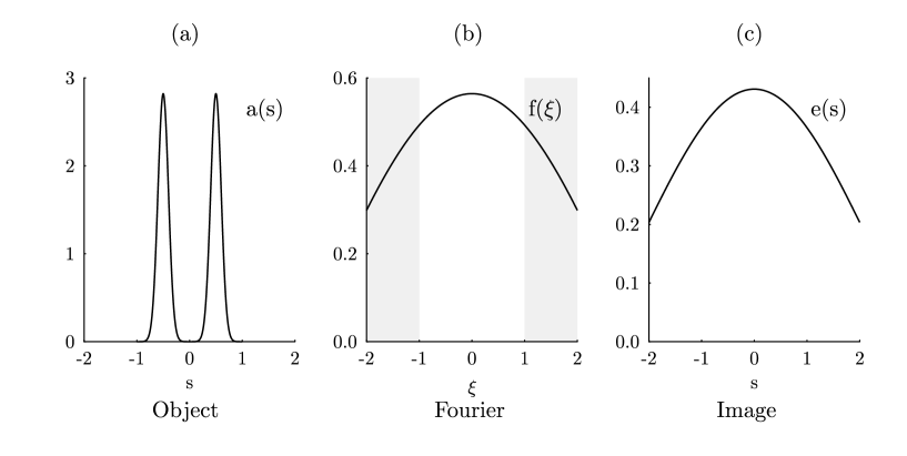
Figure 2: Double-peak object $a(s)$ used in numerical simulations (a), its spatial Fourier spectrum $f(\xi)$ in the pupil plane (b), and the image $e(s)$ created in the image plane (c). Grey area shows the part of the spatial spectrum absorbed by the opaque area of the pupil.

In Fig. 2a we have plotted the normalized input object $a(s)/\sqrt{\langle{\hat{N}}\rangle}$, in Fig. 2b - its spatial Fourier spectrum $f(\xi)$ in the pupil plane, and in Fig. 2c - the output image $e(s)$ in the image plane. Comparing the input object with its image one can clearly see that it is impossible to resolve two Gaussian peaks in the image plane according to the Rayleigh criterion. In Fig. 2b we have shown by the grey color the opaque area of the pupil. The part of the spatial Fourier spectrum of the object in this area is absorbed and therefore cannot be detected by the CCD camera placed in the pupil plane. Below we shall illustrate the reconstruction of these absorbed Fourier components by the technique of the prolate functions.

For numerical simulations we had to evaluate two sets of prolate spheroidal functions, $\varphi_{k}(s)$, defined on the interval $|s|\leq 1$, and $\psi_{k}(s)$ defined for all $s$, $-\infty<s<\infty$. The first set is necessary for decomposition of the input object $a(s)$, while the second one is needed for reconstruction of the spatial Fourier spectrum $f^{(r)}(\xi)$. For numerical calculations of $\varphi_{k}(s)$ we have used the algorithm from Ref. Xiao01 . In this algorithm the prolate functions $\varphi_{k}(s)$ are evaluated as the series with the Legendre polynomials $P_{k}(s)$,

$$\varphi_{n}(s)=\sum_{k=0}^{\infty}\gamma^{(n)}_{k}\sqrt{k+\frac{1}{2}}P_{k}(s),\quad\quad|s|\leq 1.$$ (23)

The coefficients $\gamma^{(n)}_{k}$ are found as the eigenvectors of the symmetric matrix $A$ with the following nonzero elements,

$$A_{k,k}=k(k+1)+c^{2}\frac{2k(k+1)-1}{(2k+3)(2k-1)},$$ (24)

$$A_{k,k+2}=A_{k+2,k}=c^{2}\frac{(k+2)(k+1)}{(2k+3)\sqrt{(2k+1)(2k+5)}},$$ (25)

for all $k=0,1,2\dots$

We have written a numerical program in MATHEMATICA which implements this algorithm. The advantage of this method is that it does not require the direct solution of the eigenproblem for $\varphi_{k}(s)$ and $\lambda_{k}$ which is unstable due to the rapid decrease of the eigenvalues. This algorithm allows us to calculate for $c=1$ at least $17$ first prolate functions in spite of the fact that the eigenvalues of the higher order functions become extremely small (for example, $\lambda_{17}=4.183\times 10^{-50}$). In Fig. 3 we show the first 17 prolate functions $\varphi_{k}(s)$ evaluated by our numerical program.

For numerical calculation of the second set of the prolate spheroidal functions, $\psi_{k}(s)$, we have used the following property of the Legendre polynomials ( see Eq. (10.1.14) in Ref. Abramowitz70 ),

$$\int_{-1}^{1}P_{n}(s)e^{-ics\xi}ds=2i^{n}j_{n}(\xi),$$ (26)

where $j_{n}(s)$ is the spherical Bessel function of the first order Abramowitz70 . Using this equation we can easily obtain the following representation of $\psi_{n}(\xi)$,

$$\psi_{n}(\xi)=\sqrt{\frac{2c}{\pi}}i^{n}\sum_{k=0}^{\infty}(-i)^{k}\gamma^{(n)}_{k}\sqrt{k+\frac{1}{2}}j_{k}(c\xi),\quad\quad-\infty<\xi<\infty.$$ (27)

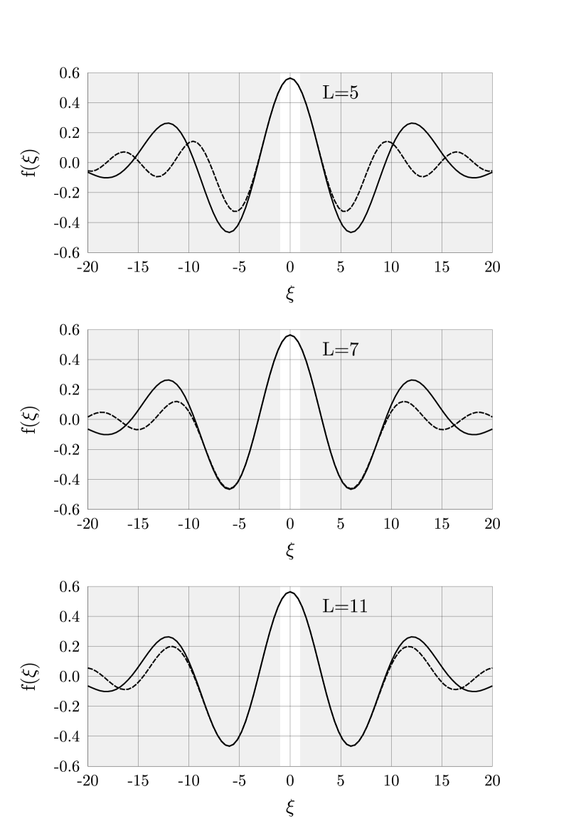
Figure 4: Exact spatial Fourier spectrum of the object from Fig. 2a (solid line), and the spectra reconstructed with $L=5,7$ and 11 prolate functions (dashed lines). Here and in Fig. 5 grey area indicates the absorbed part of the spatial spectrum.

We illustrate the result of reconstruction of the spatial Fourier spectrum of the input object in Fig. 4. In this figure we show the exact spatial Fourier spectrum of the input object, drown by a solid line, as a function of dimensionless coordinate $\xi$ in the pupil plane. Only part of this spectrum within the transmission area of the pupil, $|\xi|\leq 1$, is transmitted to the image plane. The spatial Fourier harmonics in the opaque area of the pupils, shown by grey color, are absorbed. This is a reason of very large diffraction spread in the image plane shown in Fig. 2c. The dashed lines in Fig. 4 correspond to the spatial Fourier spectrum of the reconstructed object with $L=5,7$ and 11 prolate functions. One can see that the reconstructed spectrum approaches the exact one for ever higher spatial frequencies $|\xi|$ as the number of prolate functions increases.

With 7 prolate functions two spectra are very close to each other for spatial frequencies $|\xi|\leq 8$. This corresponds to a super-resolution factor of 8 over the Rayleigh limit.

III.2 Reconstruction of objects with quantum fluctuations

For numerical simulations of quantum fluctuations we have chosen a $c$-number representation of the quantum mechanical operators $\hat{a}_{k}$ and $\hat{b}_{k}$ in Eq. (14) corresponding to the antinormal ordering of the creation and annihilation operators. In this representation the operators $\hat{a}_{k}$ and $\hat{b}_{k}$ become the $c$-number Gaussian stochastic variables $\alpha_{k}$ and $\beta_{k}$ respectively, which we shall write as

$$\alpha_{k}=a_{k}+\delta\alpha_{k},\quad\quad\beta_{k}=\delta\beta_{k}.$$ (28)

Here $a_{k}=\langle\hat{a}_{k}\rangle$ is the mean value of the field coefficients in the object area, and $\delta\alpha_{k}$ and $\delta\beta_{k}$ are the stochastic Gaussian fluctuations. Note that the mean values $\langle\hat{b}_{k}\rangle$ are zero because the classical field component outside the object vanish. We have chosen the antinormally-ordered representation because it remains valid even in the case of the multimode squeezed state of light field at the input of the scheme.

We introduce the quadrature components of the fluctuations $\delta\alpha_{k}$ and $\delta\beta_{k}$ as follows,

$$\delta\alpha_{k}=\delta X^{\alpha}_{k}+i\delta Y^{\alpha}_{k},\quad\quad\delta\beta_{k}=\delta X^{\beta}_{k}+i\delta Y^{\beta}_{k}.$$ (29)

When the input light is in the coherent state in the object area and in the vacuum state outside, the correlation functions of the quadrature fluctuations are equal to

$$\langle\delta X^{\mu}_{k}\delta X^{\mu}_{k^{\prime}}\rangle=\langle\delta Y^{\mu}_{k}\delta Y^{\mu}_{k^{\prime}}\rangle=\frac{1}{4}\delta_{kk^{\prime}},$$ (30)

with $\mu=\alpha,\beta$.

If instead of coherent light we use the multimode squeezed light for illumination of the object and multimode squeezed vacuum in the area outside with subsequent homodyne detection at the pupil plane, these correlation functions become

$$\langle\delta X^{\mu}_{k}\delta X^{\mu}_{k^{\prime}}\rangle=\frac{1}{4}e^{-2r}\delta_{kk^{\prime}}\quad\quad\langle\delta Y^{\mu}_{k}\delta Y^{\mu}_{k^{\prime}}\rangle=\frac{1}{4}e^{2r}\delta_{kk^{\prime}},$$ (31)

where $r$ is the squeezing parameter. In these formulas we have assumed that the input light is amplitude-squeezed and for simplicity have chosen the same squeezing parameter for all the essential modes that are used in the decomposition of the reconstructed object.

The relative value of quantum fluctuations depends on the signal-to-noise ratio in the input object which for the light in a coherent state is determined by the total mean number of photons passed through the object area during the observation time. For example, for a laser beam with $\lambda=1064$ nm and optical power of 1 mW, and observation time of 1 ms we obtain the mean photon number of $\langle{\hat{N}}\rangle=5.3\cdot 10^{12}$.

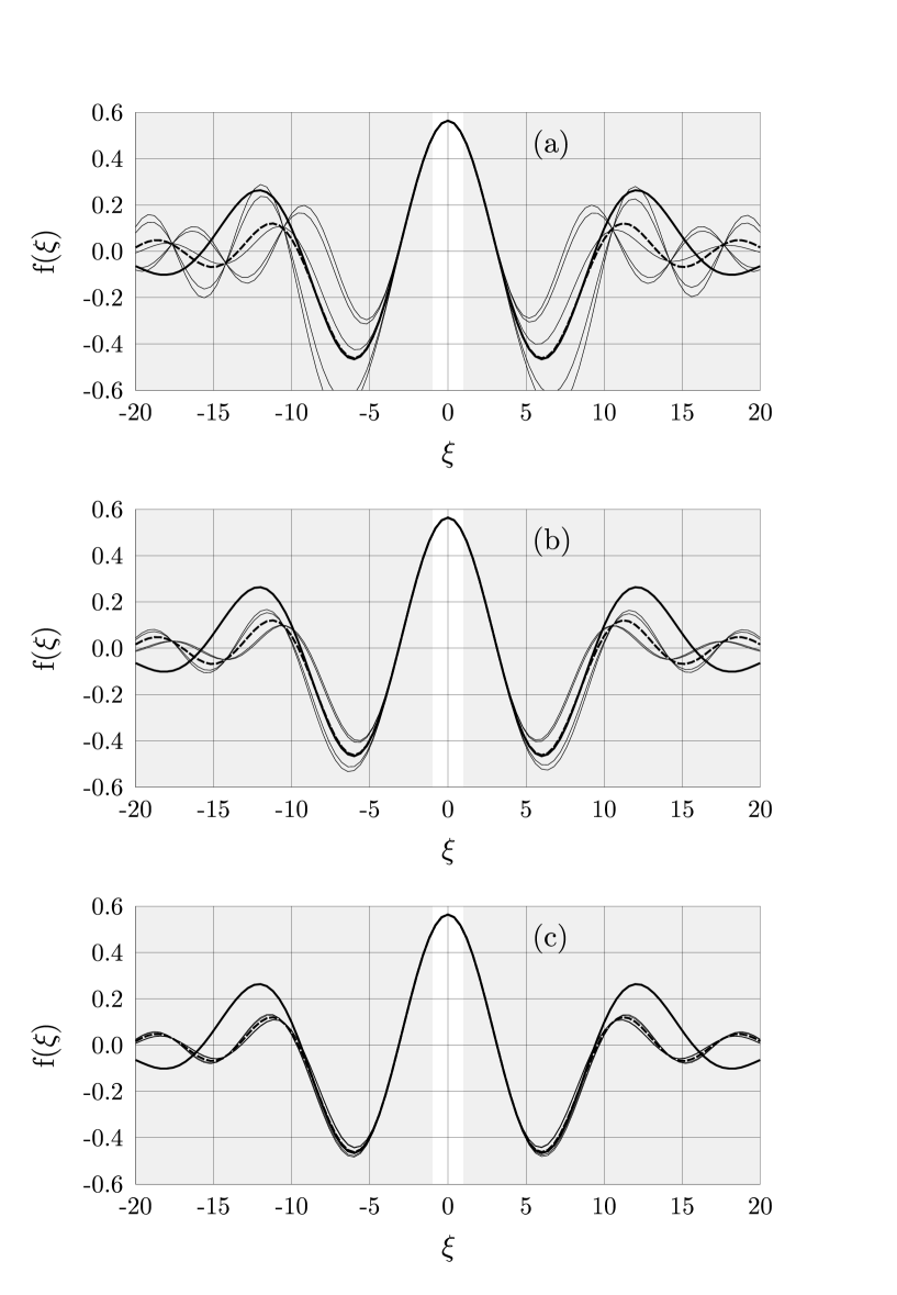
Figure 5: Exact spatial Fourier spectrum of the object from Fig. 2a (solid line), the reconstructed spectrum with $L=7$ prolate functions (dashed lines), and five random Gaussian realizations of the reconstructed spectrum with $L=7$ prolate functions (thin lines); (a) coherent light with mean total photon number $\langle{\hat{N}}\rangle=10^{12}$, (b) coherent light with $\langle{\hat{N}}\rangle=10^{13}$, and (c) squeezed light with $\langle{\hat{N}}\rangle=10^{12}$ and $\exp(r)=10$.

In Fig. 5a we have shown the results of reconstruction of the spatial Fourier spectrum of the object from Fig. 2a when quantum fluctuations of a coherent state are taken into account. The solid line gives the exact spatial Fourier spectrum of the object. As in Fig. 4 the grey area shows the absorbing part of the pupil. We use 7 prolate functions and the mean photon number in the input object is taken $\langle{\hat{N}}\rangle=10^{12}$. The five thin lines correspond to the five random Gaussian realizations of the quantum fluctuations in the coherent state of $\hat{a}_{k}$ and the vacuum fluctuations of $\hat{b}_{k}$. The dashed line corresponds to the reconstructed spectrum with 7 prolate functions without noise. One can observe that the role of quantum fluctuations becomes more and more important as one goes to the higher and higher spatial frequencies where the random realizations of the Fourier spectra deviate more and more from the mean value given by the dashed line.

In Fig. 5b we have increased the total mean value of photons to $\langle{\hat{N}}\rangle=10^{13}$. This corresponds to an increased signal-to-noise ratio in the input object and should allow for better super-resolution. This is illustrated in Fig. 5b by reduced deviation of the random realizations from the mean value of the spectrum a compared to Fig. 5a.

The same result can be achieved by using multimode squeezed light instead of increasing the power of the source illuminating the object. This is illustrated in Fig. 5c where we have used $\langle{\hat{N}}\rangle=10^{12}$ as in the Fig. 5a, but have considered the light in a multimode squeezed state with the squeezing parameter $e^{r}=10$ instead of the coherent state. As the result the fluctuations in the higher spatial frequencies are reduced that gives better super-resolution.

In next section we shall give a quantitative characteristic of super-resolution as a function of the signal-to-noise ratio.

IV Point-spread function for super-resolving reconstruction of objects

In modern classical optics the resolution of an optical system is characterized not by the two-point Rayleigh resolution criterion, but in terms of its spatial transmission bandwidth. A typical optical system has a finite band of spatial frequencies that are transmitted through the system up to some cut-off frequency determined by the size of the system pupil. The optical system is then said to be bandlimited or diffraction-limited since diffraction effects on its pupil are responsible for finite resolution.

A coherent diffraction-limited imaging system in classical optics can be described by a linear equation relating the complex amplitude $a(s)$ of an input object with the complex amplitude $e(s)$ of the image Bertero96 ,

$$e(s)=\int_{-\infty}^{\infty}h(s,s^{\prime})a(s^{\prime})ds^{\prime},$$ (32)

The impulse response function $h(s,s^{\prime})$ that appears in this integral equation represents the image at point $s$ in the image plane from a point-source at point $s^{\prime}$ in the object plane. For translationally invariant or isoplanatic systems the impulse response depends only on the difference $s-s^{\prime}$ and the integral in (32) becomes convolution,

$$e(s)=\int_{-\infty}^{\infty}h(s-s^{\prime})a(s^{\prime})ds^{\prime}.$$ (33)

In optics, the impulse response $h(s-s^{\prime})$ is usually called the point-spread function (PSF) of the system, and its Fourier transform the transfer function (TF). For bandlimited optical systems the transfer function is identically zero outside the transmission band of the system. Super-resolution is defined as technique of restoring the spatial frequencies of the object outside the transmission band Bertero96 . It is important to underline that in case when the object and the image fields are related by the convolution (33), super-resolution is impossible. To achieve super-resolution one needs some a priori information about the input object. In our case the a priori information is the assumption that the object has finite size. With this assumption Eq. (33) in dimensionless coordinates becomes Kolobov00 ,

$$e(s)=\int_{-1}^{1}h(s-s^{\prime})a(s^{\prime})ds^{\prime},$$ (34)

with the imaging PSF $h(s-s^{\prime})$ given by

$$h(s-s^{\prime})=\frac{\sin[c(s-s^{\prime})]}{\pi(s-s^{\prime})}.$$ (35)

For the reconstruction process we can write similar relation between the reconstructed field operator ${\hat{a}}^{(r)}(s)$ and the object field operator ${\hat{a}}(s)$. Using an operator-valued equivalent of Eq. (19) together with Eq. (14) we arrive at the following result,

$$\hat{a}^{(r)}(s)=\int_{-1}^{1}h^{(r)}(s,s^{\prime})\hat{a}(s^{\prime})ds^{\prime}+\sum_{k=0}^{L-1}\sqrt{\frac{1-\lambda_{k}}{\lambda_{k}}}\hat{b}_{k}\varphi_{k}(s).$$ (36)

Here the reconstruction point-spread function $h^{(r)}(s,s^{\prime})$ is given by

$$h^{(r)}(s,s^{\prime})=\sum_{k=0}^{L-1}\varphi_{k}(s)\varphi_{k}(s^{\prime}).$$ (37)

As seen from this equation, the form of the reconstruction PSF and, in particularly, its width depends on the number of terms $L$ in the sum. When this number grows infinitely, $L\to\infty$, the reconstruction PSF tends to $\delta$-function,

$$\lim_{L\to\infty}h^{(r)}(s,s^{\prime})=\sum_{k=0}^{\infty}\varphi_{k}(s)\varphi_{k}(s^{\prime})=\delta(s-s^{\prime}),$$ (38)

and we have unlimited super-resolution. However, this ideal situation is never realized practically due to the second term in Eq. (36) which grows infinitely when $L\to\infty$. Thus, Eq. (36) is a good illustration of the statement that the ultimate limit of super-resolution in the reconstructed object is given not by diffraction but by the quantum fluctuations of light represented by the second term.

The number $L$ of terms in the sum (37) which determines the width of the reconstruction PSF, depends on the signal-to-noise ratio in the input object. To obtain the maximum $L$ we shall compare the signal-to-noise ratio in the input object to that in the reconstructed object. As follows from Eq. (36) with increasing $L$ the signal-to-noise ratio in the reconstructed object deteriorates. We shall assume that reconstruction of the object is possible until the limit when the signal-to-noise ratio in the reconstructed object becomes unity.

Let us define the singal-to-noise ratio in the input object as Kolobov95

$$R=\frac{\langle{\hat{N}}\rangle^{2}}{\langle(\Delta{\hat{N}})^{2}\rangle},$$ (39)

where

$$\langle{\hat{N}}\rangle=\int_{-1}^{1}\langle{\hat{a}}^{{\dagger}}(s){\hat{a}}(s)\rangle ds,$$ (40)

is the total mean number of photons in the input object, and $\langle(\Delta{\hat{N}})^{2}\rangle$ - its variance. Similarly we define the signal-to-noise ratio $R^{(r)}$ in the reconstructed object as

$$R^{(r)}=\frac{\langle{\hat{N}^{(r)}}\rangle^{2}}{\langle(\Delta{\hat{N}^{(r)}})^{2}\rangle},$$ (41)

where the mean number of photons in the reconstructed object is given by

$$\langle{\hat{N}^{(r)}}\rangle=\int_{-1}^{1}\langle{\hat{a}}^{(r){\dagger}}(s){\hat{a}^{(r)}}(s)\rangle ds.$$ (42)

The deterioration of the signal-to-noise ratio in the reconstructed object can be described by the noise figure $F$,

$$F=\frac{R}{R^{(r)}},$$ (43)

that is commonly used in the literature about amplifiers. Because the signal-to-noise ratio $R^{(r)}$ in the reconstructed object is always smaller than that in the input object, the noise figure is always larger than unity. If we assume that the minimum value of $R^{(r)}$ that allows for reconstruction of the object is unity, this gives us the maximum noise figure $F_{\rm max}=R$ corresponding to the maximum super-resolution.

Let us consider an input object in a coherent state, so that $\langle{\hat{a}}(s)\rangle=a(s)$, $\langle{\hat{a}}^{{\dagger}}(s){\hat{a}}(s)\rangle=|a(s)|^{2}$, $\langle{\hat{a}}^{{\dagger}}(s){\hat{a}}^{{\dagger}}(s^{\prime}){\hat{a}}(s^{\prime}){\hat{a}}(s)\rangle=|a(s)|^{2}|a(s^{\prime})|^{2}$. It is easy to show that in this case the input signal-to-noise ratio $R$ is equal to the mean total photon number in the input object,

$$R=\langle{\hat{N}}\rangle=\int_{-1}^{1}|a(s)|^{2}ds.$$ (44)

On the other hand, for the signal-to-noise ratio $R^{(r)}$ in the reconstructed object in this case we obtain the following result

$$R^{(r)}=\Bigl{(}\sum_{k=0}^{L-1}|a_{k}|^{2}\Bigr{)}^{2}/\Bigl{(}\sum_{k=0}^{L-1}\frac{|a_{k}|^{2}}{\lambda_{k}}\Bigr{)},$$ (45)

where $a_{k}$ are the coefficients of decomposition of $a^{(r)}(s)$ over the prolate functions $\varphi_{k}(s)$ in Eq. (19).

As follows from Eq. (45), the signal-to-noise ratio $R^{(r)}$ and, therefore, the noise figure $F$ depend on the shape of the input object. For numerical evaluation of the super-resolution factor as a function of the total mean number of photons in the input object we have taken a narrow rectangular object placed at the origin $s=0$,

$$a_{\epsilon}(s)=\left\{\begin{array}[]{cl}\displaystyle{\sqrt{\frac{\langle{\hat{N}}\rangle}{\epsilon}}}&\quad|s|\leq\epsilon/2,\\ 0&\quad|s|>\epsilon/2,\\ \end{array}\right.$$ (46)

Taking the width $\epsilon$ of this object ever smaller we arrive at a point-like source, while keeping the total number of photons constant and equal to $\langle{\hat{N}}\rangle$. Such a point-like object gives us the reconstruction PSF $h^{(r)}(0,s)$ at the output.

The degree of super-resolution in the reconstructed object can be characterized by the ratio of the width of the diffraction-limited imaging PSF to the width of the reconstruction PSF. In Fig. 6 we have shown the imaging PSF $h(s)$ and the reconstruction PSF $h^{(r)}(0,s)$ for $L=7$ normalized to unity at their maxima. To define the super-resolution factor we shall introduce the half-widths $W$ and $W_{L}$ of these two PSF measured at their half-maxima. Then we define the super-resolution factor $S$ as the ratio of $W$ to $W_{L}$,

$$S=\frac{W}{W_{L}}.$$ (47)

For the example given in Fig. 6 these half-widths are equal to $W=1.895$, $W_{L}=0.252$, and $S=7.5$.

In Fig. 7 we have plotted the super-resolution factor $S$ as a function of the total mean number of photons $\langle{\hat{N}}\rangle$ in the input object for the case of coherent light and multimode squeezed light. As seen from this figure, for the same mean number of photons multimode squeezed light provides higher super-resolution that the coherent light.

V Discussion and prospectives

In this paper we have investigated analytically and numerically the quantum limits of super-resolution in reconstruction of optical objects from the diffraction-limited images. We assume that such a reconstruction is performed electronically from the data collected in a homodyne detection of images by means of a CCD camera placed either in the image plane or in the Fourier plane. We call the first situation super-resolving microscopy and the second - super-resolving Fourier-microscopy. In Section II we have presented the quantum theory of the latter.

From our numerical simulations in Sections III and IV we conclude that a priori information about the finite size of the input object allows one to obtain significant super-resolution in the reconstructed object over the classical Rayleigh limit. For classical noise-free objects we have demonstrated a possibility to achieve super-resolution of factor 8 over the Rayleigh limit. When quantum fluctuations in the object are taken into account, the degree of super-resolution depends on the signal-to-noise ratio in the input object. When the object is illuminated by the light in a coherent state, this signal-to-noise ratio is given by the mean total number of photons during the observation time. We have quantitatively defined the super-resolution factor as a ratio of widths of the imaging and reconstruction point-spread functions. We have numerically evaluated this super-resolution factor as a function of the mean total number of photons for the coherent light and multimode squeezed light. For the same mean number of photons multimode squeezed light allows to achieve higher super-resolution than the coherent light.

As future prospectives for further development of the theory presented in this paper we would like to mention the problem of read-out of binary information from optical discs, like CD and DVD, or optical memory. The storage density for the optical discs currently is limited by the spot size of the diffraction-limited focussed light beam. One possibility of increasing the storage density would be an attempt to put several bits of information inside the diffraction-limited light spot with subsequent super-resolution in the read-out of this information. In this case the amount of a priori information is clearly superior to the case considered in present article since for finite number of bits inside the laser spot one has a finite possible combination of light patterns. Therefore, one would expect higher potential of super-resolution in read-out of binary information as compared to the situation that we have investigated here. In the context of the problem of read-out of optical discs one would have to generalize our theory to optical systems with high numerical apertures which is usually the case for the systems of the optical data storage.

This work was supported by the Project QUANTIM (IST-200-26019) of the European Union.

Figure 1: Optical scheme of one-dimensional coherent diffraction-limited imaging.

Figure 3: Examples of the prolate spheroidal functions $\varphi_{k}(s)$ and the corresponding eigenvalues $\lambda_{k}$ calculated using our numerical program.

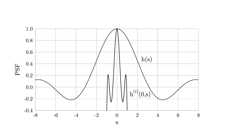
Figure 6: Diffraction-limited imaging point-spread function $h(s)$ and the reconstruction point-spread function $h^{(r)}(0,s)$ using 7 prolate functions.

Figure 7: Super-resolution factor $S$ as a function of the total mean number of photons $\langle{\hat{N}}\rangle$ for coherent light (solid line, and multimode squeezed line with $\exp(r)=10$ (dashed line).

References

- (1) M. I. Kolobov, Rev. Mod. Phys. 71, 1539 (1999).
- (2) L. A. Lugiato, A. Gatti, and E. Brambilla, J. Opt. B: Quantum Semiclass. Opt. 4, 176 (2002).
- (3) S. Kamimura, Appl. Opt. 26, 3425 (1987).
- (4) N. Treps, N. Grosse, W. P. Bowen, C. Fabre, H.-A. Bachor, and P. K. Lam, Science 301, 940 (2003).
- (5) M. I. Kolobov and C. Fabre, Phys. Rev. Lett. 85, 3789 (2000).
- (6) I. V. Sokolov and M. I. Kolobov, Optics Letters 29, 703 (2004).
- (7) P. Scotto, P. Colet, M. San Miguel, and M. I. Kolobov, in Proceedings of the European Quantum Electronics Conference EQEC 2003, Munich, (2003).
- (8) M. I. Kolobov, C. Fabre, P. Scotto, P. Colet, and M. San Miguel, in Coherence and Quantum Optics VIII, N. Bigelow, J. H. Eberly, C. R. Stroud, and I. A. Walmsley, eds. (Plenum, New York, 2003).
- (9) D. Slepian and H. O. Pollak, Bell System Techn. J. 40, 43 (1961).
- (10) B. R. Frieden, in Progress in Optics, Vol. IX, E. Wolf, ed. (North-Holland, Amsterdam, 1971), pp. 311-407.
- (11) H. Xiao, V. Rokhlin and N. Yarvin, Inverse Problems, 17, 805 (2001).
- (12) M. Abramowitz and I. A. Stegun, Handbook of Mathematical Functions, 9th ed. (Dover, New York, 1970).
- (13) M. Bertero, and C. De Mol, in Progress in Optics Vol. XXXVI, edited by E. Wolf (North-Holland, Amsterdam, 1996), p. 129.
- (14) M. I. Kolobov and L. A. Lugiato, Phys. Rev. A 52, 4930 (1995).