Thermal effects on quantum communication through spin chains
A.Bayat,       V. Karimipour

Department of Physics, Sharif University of Technology,

P.O. Box 11365-9161,

Tehran, Iran

We study the effect of thermal fluctuations in a recently proposed protocol for transmission of unknown quantum states through quantum spin chains. We develop a low temperature expansion for general spin chains. We then apply this formalism to study exactly thermal effects on short spin chains of four spins. We show that optimal times for extraction of output states are almost independent of the temperature which lowers only the fidelity of the channel. Moreover we show that thermal effects are smaller in the anti-ferromagnetic chains than the ferromagnetic ones.

1 Introduction

One of the basic ingredients of quantum communication is the transport of a known or unknown quantum state from one point to another [1]. Recently it has been shown that quantum spin chains can act as channels for the efficient [2, 3, 4] or perfect [5, 6] transfer of quantum states. Of particular interest to us here is the works reported in [2, 3]. It has been shown that this scheme may be used for linking several small quantum processers in large scale quantum computing. In this scheme, an $N$-site ferromagnetic Heisenberg spin chain placed in a magnetic field, plays the role of the quantum channel. The spins of the channel are numbered from $1$ to $N$. It is assumed that this chain is in its ground state, $|-,-,\cdots-\rangle$, where $|-\rangle$ denotes the state of a spin in the negative $z$ direction and the magnetic field points to the positive $z$ direction. One then adds a spin or qubit to the left hand side of this channel labeled by zero, which is in an unknown state $|\phi\rangle$ (figure 1-a). The state of this qubit is to be transmitted with a high fidelity to the right hand side, by the natural time evolution of the chain.
In this way one may circumvent a problem which exists in quantum computer implementation namely the difficulty of switching on and off between spins[7, 8].

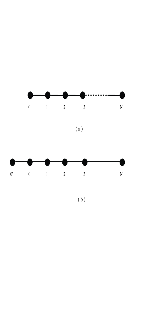
Figure 1: a-An unknown quantum state $|\phi\rangle$ is placed at site $0$ of the chain and is transported to site $N$ by the dynamics of the spin chain. b- The entanglement of a Bell state $|\phi^{+}\rangle=\frac{1}{\sqrt{2}}(|0,0\rangle+|1,1\rangle)$ placed at sites $0^{\prime}$ and $0$ develops into the entanglement of sites $0^{\prime}$ and $N$.

The Hamiltonians governing the interaction of the spins in the channel and the full chain are respectively

$$H_{c}=-J\sum_{i=1}^{N-1}{\bf\sigma}_{i}\cdot{\bf\sigma}_{i+1}+B\sum_{i=1}^{N}\sigma_{z,i},$$ (1)

and

$$H=-J\sum_{i=0}^{N-1}{\bf\sigma}_{i}\cdot{\bf\sigma}_{i+1}+B\sum_{i=0}^{N}\sigma_{z,i},$$ (2)

where the subscript ”c” on $H$ stands for the channel. If at time $t=0$ the qubit $0$ is placed to the left of the chain then the evolution of the Heisenberg chain carries the state of this qubit to the rightmost spin $N$ where one extracts the state with a rather high fidelity, provided that one extracts the state at an optimal time.
It has been shown in [2] that one can transmit quantum states with a high fidelity ranging from $F=1$ for $N=4$ to a value exceeding $0.9$ for $N=7,10,11,13$ and $14$. The fidelity generally decreases with increasing the length of the channel exceeds the classical value of $F=2/3$ for $N\approx 80$ which holds for classical transmission of quantum states[9].
One can also use this channel for transmission of entanglement in the following way [2]. One places two maximally entangled spins labeled $0^{\prime}$ and $0$ to the left of the chain (figure 1-b) and evolution of the chain after a suitable lapse of time entangles the spin $0^{\prime}$ to the rightmost spin $N$ here it is assumed that only the spin $0$ is coupled to the channel. In this way two distant spins can be entangled which can later be used for implementation of other quantum protocols like teleportation [10].

The formalism of [2] requires that the spins of the channel be ideally aligned in the direction opposite to that of the magnetic field. This ideal situation is however achievable only at zero temperature or in very strong magnetic fields where thermal fluctuations are not large enough to populate excited states, i.e. (when $B/kT>>1$). On the other hand increasing the magnetic field may lower the quality of the channel since a high magnetic field tends to align the spins and will generally dominate the interaction between the spins which is essential for the working of the channel.
Moreover when one uses this channel once and extracts the state at the right hand site, the initial state of the channel turns into a mixed state. Before using the channel for another round of transmission the initial state of the channel should be restored, for example by cooling to low enough temperatures. It is plausible to assume that multiple uses of the channel may heat it up to temperatures in which not only the ground state but also some of the excited states are also populated.

In view of these considerations it is desirable to study the effect of thermal fluctuations on such a quantum channel. This is the problem that we want to address in this paper. Thus we want to generalize the protocol of [2] to the case where the initial state of the channel is not the ground state but a thermal state given by a thermal density matrix.
This enables us to to see the effect of the ambient temperature on the feasibility of the protocol, and the quantitative effect that temperature has on the fidelity of transmission of states and distribution of entanglement.
We will derive a low temperature expansion through which we can study the effect of temperature to any desired degree of accuracy by keeping appropriate number of terms in the expansion.
In a sequel to this paper we will study long chains of arbitrary number of spins at low temperatures. This study can be done only numerically. In this paper however we will study exactly thermal effects on a short chain of four spins. The advantage of studying this short chain is that we can obtain the spectrum completely and hence can compare the two cases of ferromagnetic and antiferromagnetic chains.

The structure of this paper is as follows: In section 2 we set up the general formalism and will develop low temperature expansions for the expressions of fidelity and entanglement. In section 3 we derive general expressions for entanglement of endpoints of the chain at arbitrary temperatures. In section 4 we study exactly the specific example of a short chain of only $4$ spins where we present our basic results in figures (2 to 5).

2 Low temperature expansion of the fidelity

We consider the interaction between the spins to be nearest neighbor and of Heisenberg type. The spins also interact with an external magnetic field. We should emphasize that much of what we derive in this section do not depend on a specific form of the Hamiltonian. We assume that the initial state of the channel is

$$\rho_{th}=\frac{e^{-\beta H_{c}}}{Z}=\sum_{\alpha}\frac{e^{-\beta E_{\alpha}}}{Z}|\alpha\rangle\langle\alpha|,$$ (3)

where $|\alpha\rangle$’s and $E_{\alpha}$’s are respectively the eigenstates and eigenenergies of the channel Hamiltonian (1). Here $Z$ is the partition function of the channel $Z:=tr(e^{-\beta H_{c}})$.
At time $t=0$ we place the $0$-th spin which is in an unknown pure state $\rho_{0}=|\phi\rangle\langle\phi|$ to the left of this channel. The initial state of the whole chain will be given by $\rho_{0}\otimes\rho_{th}$ which evolves to

$$\rho(t)=e^{-iHt}(\rho_{0}\otimes\rho_{th})e^{iHt},$$ (4)

where $H$ is now the Hamiltonian of the full chain (2).
The state of the $N$-th spin after time $t$ will be given by

$$\rho_{N}(t)=tr_{\hat{N}}(e^{-iHt}(\rho_{0}\otimes\rho_{th})e^{iHt}),$$ (5)

where $\hat{N}$ means that we take the trace over all sites except the $N$-th site. We can now derive an operator sum representation for the transformation of the state of the leftmost qubit $\rho(0):=|\phi\rangle\langle\phi|$ to the state of the rightmost qubit $\rho_{N}(t)$. To do this we use (5) to compute an element of $\rho_{N}(t)$ as follows, where we use the index $I$ to run over a complete set of states $\{|I\rangle\}$ for the Hilbert space of part of the total chain from site $0$ to site $N-1$, and the index $\alpha$ is to run over the eigenstates of the channel Hamiltonian:

$$\langle k|\rho_{N}(t)|l\rangle = \sum_{I}\langle I,k|e^{-iHt}(\rho_{0}\otimes\rho_{th})e^{iHt}|I,l\rangle$$ (6)

$$= \sum_{I,j,m,\alpha,\beta}\langle I,k|e^{-iHt}|j,\alpha\rangle\langle j,\alpha|(\rho_{0}\otimes\rho_{th})|m,\beta\rangle\langle m,\beta|e^{iHt}|I,l\rangle$$ (7)

$$= \sum_{I,j,m,\alpha}\langle I,k|e^{-iHt}|j,\alpha\rangle{\rho_{0}}_{j,m}\langle m,\alpha|e^{iHt}|I,l\rangle\frac{e^{-\beta E_{\alpha}}}{Z}.$$ (8)

Defining a collection of two by two matrices $M_{I,\alpha}$ with elements

$$\langle k|M_{I,\alpha}|j\rangle:=\frac{e^{\frac{-\beta E_{\alpha}}{2}}}{\sqrt{Z}}\langle I,k|e^{-iHt}|j,\alpha\rangle$$ (9)

we find the following Kraus decomposition [11, 12] for $\rho_{N}(t)$,

$$\rho_{N}(t)=\sum_{I,\alpha}M_{I\alpha}\rho_{0}M^{\dagger}_{I\alpha}.$$ (10)

Note that in general the number of elements in this decomposition, i.e. the number of matrices $M_{I,\alpha}$ is huge. In fact this number is equal to the number of different choices for the pair of indices $(I,\alpha)$, which equals $2^{2N}$. In principle there are many operator sum representations for a superoperator and the number of kraus operators for a qubit can be reduced to $4$ [11, 12], however the present form has the advantage that it is suitable for a low temperature expansion of the fidelity of the channel. Note also that even in the present form symmetry arguments highly restricts the number of nonzero matrices as we will see in the sequel.

The fidelity of this out-state $\rho_{N}(t)$ with the in-state $\rho_{0}$ is given by

$$F=\sum_{I,\alpha}tr(\rho_{0}M_{I\alpha}\rho_{0}M^{\dagger}_{I\alpha}).$$ (11)

We are interested in the fidelity averaged over all the initial input states, that is

$$\overline{F}=\frac{1}{4\pi}\int Fd\Omega,$$ (12)

where the integral is taken over the surface of the Bloch sphere. This integral can further be simplified by using the following easily verified identity

$$tr(\rho_{0}A\rho_{0}B)=tr((A\otimes B)S(\rho_{0}\otimes\rho_{0}))$$ (13)

where $S$ is the swap operator with elements $S_{ij,kl}=\delta_{il}\delta_{jk}$. We now write $\rho_{0}$ as $\rho_{0}=\frac{1}{2}({\bf 1}+{\bf n}\cdot{\sigma})$ and use the identity $\frac{1}{4\pi}\int n_{i}n_{j}d\Omega=\frac{1}{3}\delta_{ij}$ to arrive at the following identity

$$\frac{1}{4\pi}\int\rho_{0}\otimes\rho_{0}d\Omega=\frac{1}{6}(\bf{1}+S),$$ (14)

which we use to rewrite $\overline{F}$ as

$$\overline{F}=\frac{1}{6}\sum_{I,\alpha}tr(M_{I\alpha}\otimes M^{\dagger}_{I\alpha}(\bf{1}+S)).$$ (15)

Using the facts that $tr((A\otimes B)S)=tr(AB)$ and $\sum_{I,\alpha}M_{I\alpha}^{\dagger}M_{I\alpha}=\bf{1}$ we find the final form of $\overline{F}$ as

$$\overline{F}=\frac{1}{3}+\frac{1}{6}\sum_{I,\alpha}|trM_{I\alpha}|^{2}.$$ (16)

Equation (16) is already in the form of a low temperature expansion for the average fidelity. The leading contribution comes from the ground state which we label as $\alpha_{0}$, the next to leading contribution comes from the first excited states and so on. Thus despite the huge number of matrices $M_{I,\alpha}$, at low temperatures one can obtain a reasonably good value of the fidelity by using only the first few terms in the expansion.

2.1 The zero temperature limit of the ferromagnetic chain

In this limit only the ground state contributes to the expansion (16). For the ferromagnetic chain the ground state is

$$|\alpha_{0}\rangle=|-,-,-,\cdots,-\rangle$$ (17)

where all the spins are down. Thus we have

$$\overline{F}=\frac{1}{3}+\frac{1}{6}\sum_{I}|trM_{I\alpha_{0}}|^{2}.$$ (18)

In (18) it appears that a set of $2^{N}$ matrices $M_{I,\alpha_{0}}$ contribute to the sum. However we show that by symmetry considerations one can reduce this number to only two. To this end we note that a general element of $M_{I,\alpha_{0}}$ can be written as follows:

$$M_{I,\alpha_{0}}(i,j)=\langle I,i|e^{-iHt}|j,-,-,-,\cdots,-\rangle.$$ (19)

In view of the symmetry $[H,J_{z}]=0$ where $J_{z}$ is the total spin in the $z$ direction, the only nonzero matrices are those in which the index $I$ is either $(-,-,-,\cdots,-)$ for which we denote the corresponding matrix by $M_{0}$, or those in which only one spin is up (e.g. in the $i$-th position $(-,-,\cdots-,+,-,\cdots,-))$ for which we denote the corresponding matrix by $M_{i}$.
Moreover the above mentioned symmetry requires that matrices be of the following form:

$$M_{0} = \left(\begin{array}[]{cc}m_{+}&0\\ 0&m_{-}\end{array}\right),$$ (22)

$$M_{i} = \left(\begin{array}[]{cc}0&0\\ m_{i}&0\end{array}\right)\hskip 28.45274pti=1\cdots N,$$ (25)

where

$$m_{+}: = \langle-,-,\cdots-,+|e^{-iHt}|+,-,-,\cdots,-\rangle,$$ (26)

$$m_{-}: = \langle-,-,\cdots-,-|e^{-iHt}|-,-,-,\cdots,-\rangle,$$ (27)

and

$$m_{i}:=\langle-,\cdots-,+,-\cdots-|e^{-iHt}|+,-,-,\cdots,-\rangle.$$ (28)

A simple calculation now shows that the following identity holds for the above types of matrices, regardless of their explicit form of matrix elements,

$$\sum_{i=1}^{N}M_{i}\rho M_{i}^{\dagger}=\textbf{M}\rho\textbf{M}^{\dagger},$$ (29)

where

$$\textbf{M}=\left(\begin{array}[]{cc}0&0\\ \sqrt{\sum_{i=1}^{N}|m_{i}|^{2}}&0\end{array}\right)\\ .$$ (30)

Thus the operator sum representation reduces to a sum with only two elements, i.e.

$$\rho_{N}(t)=M_{0}\rho_{0}M_{0}^{\dagger}+\textbf{M}\rho_{0}\textbf{M}^{\dagger}.$$ (31)

Using (18) and noting that the matrix M is traceless, we find the average fidelity at zero temperature:

$$\overline{F}=\frac{1}{3}+\frac{1}{6}|m_{+}+m_{-}|^{2}$$ (32)

For the ferromagnetic chain, the state $|-,-,\cdots,-\rangle$ is also the ground state of the full Hamiltonian and thus by shifting the zero energy of the Hamiltonian to $0$ we can set $m_{-}=1$. Thus we find

$$\overline{F}=\frac{1}{3}+\frac{1}{6}|1+m_{+}|^{2}$$ (33)

in accordance with the result of [2]. Note that our $m_{+}$ is denoted by $f_{0,N}(t)$ in [2].

3 Transfer of entanglement

We now consider how temperature affects the distribution of a maximally entangled pair through the channel. Following [2] we consider a maximally entangled pair of qubits in the state $|\Phi_{+}\rangle:=\frac{1}{\sqrt{2}}(|0,1\rangle+|1,0\rangle)$. In figure (1-b) this pair of qubits are labeled by $0^{\prime}$ and $0$.

The evolution of the chain may transform the entanglement between the pair $(0^{\prime},0)$ to the pair $(0^{\prime},N)$, thus enabling us to transport entanglement between ions or any other realization of qubits over long distances. Note that the Hamiltonian only acts on the part of the chain form $0$ to $N$. It is assumed that the qubit $0^{\prime}$ does not interact with the rest of the chain. After a time $t$, the density matrix of the pair $(0^{\prime},N)$ is easily obtained thanks to the operator sum representation (10). We find

$$\rho_{0^{\prime},N}(t)=\sum_{I,\alpha}(\mathbf{1}\otimes M_{I\alpha})(|\Phi_{+}\rangle\langle\Phi_{+})(\mathbf{1}\otimes M^{\dagger}_{I\alpha}).$$ (34)

Using the fact that

$$|\phi_{+}\rangle\langle\phi_{+}|=\frac{1}{2}\left(\begin{array}[]{cccc}0&&&\\ &1&1&\\ &1&1&\\ &&&0\\ \end{array}\right)$$ (35)

and the explicit form of the matrix elements of $M_{I,\alpha}$ as given in (9) we find after some manipulations the following low temperature expansion:

$$\rho_{0^{\prime},N}(t):=\sum_{\alpha}\frac{e^{-\beta E_{\alpha}}}{Z}\rho_{(\alpha)}(t),$$ (36)

where each $\rho_{\alpha}$ pertains to a level $\alpha$ of the spectrum of the channel and is given by

$$\rho_{(\alpha)}(t)=\left(\begin{array}[]{cccc}u^{+}_{\alpha}(t)&&&\\ &w^{+}_{\alpha}(t)&z_{\alpha}(t)&\\ &z^{*}_{\alpha}(t)&w^{-}_{\alpha}(t)&\\ &&&u^{-}_{\alpha}(t)\\ \end{array}\right)$$ (37)

where

$$u^{+}_{\alpha}(t) = \frac{1}{4}\langle 1,\alpha|(1+\sigma^{z}_{N}(t))|1,\alpha\rangle$$ (38)

$$u^{-}_{\alpha}(t) = \frac{1}{4}\langle 0,\alpha|(1-\sigma^{z}_{N}(t))|0,\alpha\rangle$$ (39)

$$w^{+}_{\alpha}(t) = \frac{1}{4}\langle 1,\alpha|(1-\sigma^{z}_{N}(t))|1,\alpha\rangle$$ (40)

$$w^{-}_{\alpha}(t) = \frac{1}{4}\langle 0,\alpha|(1+\sigma^{z}_{N}(t))|0,\alpha\rangle$$ (41)

$$z_{\alpha}(t) = \frac{1}{2}\langle 0,\alpha|\sigma^{+}_{N}(t)|1,\alpha\rangle.$$ (42)

Here the operators $\sigma^{a}_{N}(t)$ are operators in the Heisenberg picture, i.e. ($\sigma^{a}_{N}(t)=e^{iHt}\sigma^{a}_{N}e^{-iHt}$).
Thus the concurrence will have the same dependence on the correlation function as in the thermal equilibrium state [14, 15], only now the correlation functions are time dependent.

4 Exact solution for a short chain

An exact study of the thermal effects on a long chain with arbitrary number of spins is highly involved, since it requires a knowledge of all the energy eigenstates. On can study these chains only at low temperatures in which case only the ground state and the first excited states of the chain are populated. We will do this in a sequel to this paper. Here we study exactly a short spin chain of $N=3$. An exact study of a short chain has the advantage that one can compare the characteristically different behaviors of ferromagnetic and anti-ferromagnetic chains. We remind the reader that at zero temperature the channel relaxes to its ground state which for the ferromagnetic chain is a disentangled state of spins aligned with the magnetic field. This is the only case which has been studied in [2].
So we consider a three site channel with hamiltonian given by

$$H_{c}=-J({\bf s}_{1}\cdot{\bf s}_{2}+{\bf s}_{2}\cdot{\bf s}_{3})+B(s_{1z}+s_{2z}+s_{3z}).$$ (43)

The spectrum of this hamiltonian is easily obtained and it exist in the appendix.
The Hamiltonian of the full chain is now

$$H=-J({\bf s}_{0}\cdot{\bf s}_{1}+{\bf s}_{1}\cdot{\bf s}_{2}+{\bf s}_{2}\cdot{\bf s}_{3})+B(s_{0z}+s_{1z}+s_{2z}+s_{3z}).$$ (44)

Determination of the spectrum of this hamiltonian is facilitated by using the following symmetries, namely

$$[H,J_{z}]=[H,\Lambda]=[J_{z},\Lambda]=0\ \ \ {\rm and}\ \ \ \sigma_{x}^{\otimes 4}H(J,B)=H(J,-B)\sigma_{x}^{\otimes 4},$$ (45)

where $\Lambda$ is the inversion operator

$$\Lambda|s_{0},s_{1},s_{2},s_{3}\rangle=|s_{3},s_{2},s_{1},s_{0}\rangle.$$ (46)

The spectrums of the total and the channel hamiltonian are derived in the appendix. By plugging these eigenstates and eigenvalues in equations (9) and (16) one can determine the average fidelity of the output state with the input state. The fidelity is a complicated function of time, in fact it is a superposition of periodic functions with periods $\omega_{ij}:=\frac{1}{|E_{j}-E_{i}|}$ . In [2] one extracts the output state only at certain times where the fidelity reaches a maximum. Since we want to focus on the effect of temperature, we fix the magnetic field and determine the average fidelity as a function of time and temperature. The results are shown in figure (2) and (3) for ferromagnetic and anti-ferromagnetic chains respectively.

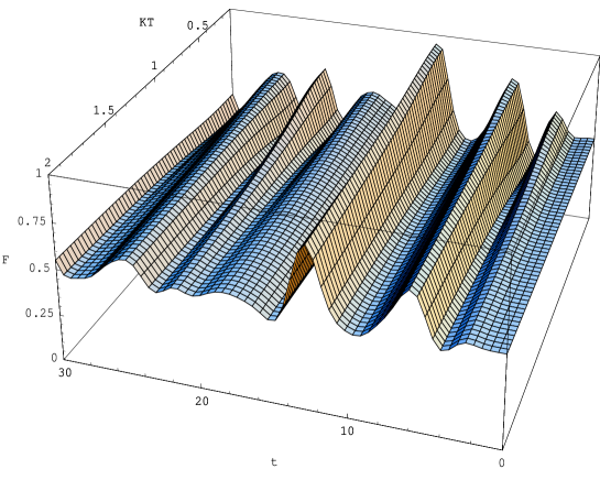
Figure 2: (Color Online) The fidelity (F) between the output and the input states averaged over all input states, as a function of $kT$ and time $t$, in a fixed magnetic field. In all the figures the fidelity $F$ and the concurrence $C$ are dimensionless and we are working in units where $KT$ and $t$ have no dimensions. In these units we have taken $B=1$ and $J=+1$ for ferromagnetic and $J=-1$ for anti-ferromagnetic chains.

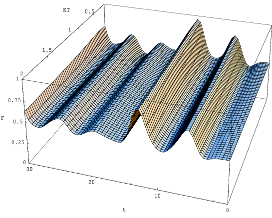
Figure 3: (Color Online) The fidelity (F) between the the output and the input states averaged over all input states, as a function of $kT$ and time (t), in a fixed magnetic field $(B=1)$, for an anti-ferromagnetic channel $(J=-1)$.

These curves show several interesting features. The first one is that the optimal time of extraction is almost independent of temperature, thus at any temperature one can tune the optimal time of extraction to be the same as that of the zero temperature. The only effect of temperature is that it decreases the fidelity. It is also seen that the optimal times when the fidelity reaches local maxima are the same for both types of chains. Moreover thermal fluctuations have much less destructive effect on the fidelity in the anti-ferromagnetic chain as compared with the ferromagnetic chain.
The difference between these two types of chains is more pronounced when we use them to transfer entanglement. We have used these two channels to transfer the maximal entanglement between the two spins $0^{\prime}$ and $0$ at the left hand side of the chain (1) to entanglement of the end points of the chains at time $t$, measured by the concurrence of the density matrix $\rho_{0^{\prime},3}$. In a fixed magnetic field, the concurrence of this density matrix [13] is a function of temperature. Figures (4) and (5) show this concurrence as a function of temperature and time for the ferromagnetic and anti-ferromagnetic chains respectively. All the previous comments apply also to this type of behavior. The striking difference is that in the anti-ferromagnetic chain, there are long intervals of time when no entanglement can be distributed in the chain regardless of the temperature, entanglement transfer is possible only in short periods of time. In fact comparison of the figures for the fidelity and concurrence shows that when the fidelity of the channel drops below the approximate value of $0.6$, it no longer can transfer any entanglement.

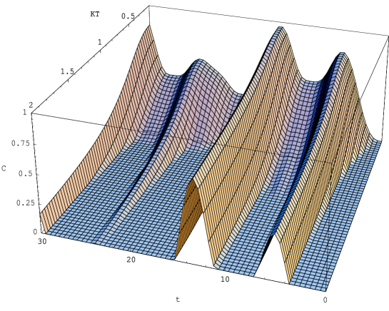
Figure 4: (Color Online) The concurrence $C$ of the state of the endpoints of the chain as a function of time $t$ and $kT$ in a fixed magnetic field for a ferromagnetic chain. Here $B=1$ and $J=1$.

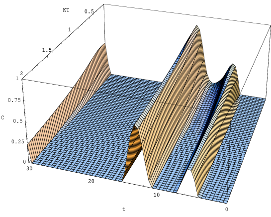
Figure 5: (Color Online)The concurrence $C$ of the state of the endpoints of the chain as a function of time $t$ and $kT$, in a fixed magnetic field $(B=1)$, for a anti-ferromagnetic chain $(J=-1)$.

5 Summary

We have studied the effect of thermal fluctuations on a recently proposed method for transportation of unknown states through quantum spin chains. We have developed a low temperature expansion which can be used to calculate this effect to a desired degree of accuracy at any given temperature. As an example we have calculated exactly the effect of thermal fluctuations on transportation of states on a short spin chain and have shown that the optimal time of extraction of transported states at the end of the chain is almost independent of temperature, the only effect of which is to lower slightly the fidelity of the output state with the input state. We have made a detailed comparison between the ferromagnetic and anti-ferromagnetic channels.

6 Acknowledgement

A. Bayat would like to thank A. T. Rezakhani for his help in drawing the figures. We also thank I. Marvian for his very constructive comments and M. Asoudeh and L. Memarzadeh for their critical reading of the manuscript.

7 Appendix :Spectrum of three and four Site Spin chain

In this appendix we collect the eigenstates and eigenvalues of the hamiltonians $H_{c}$ and $H$ shown in equations (43) and (44).
The eigenstates and eigenenergies of the channel are as follows:

$$|\alpha_{1}\rangle = |-,-,-\rangle,$$ (47)

$$|\alpha_{2}\rangle = \frac{1}{2}(|+,-,-\rangle-\sqrt{2}|-,+,-\rangle+|-,-,+\rangle,$$ (48)

$$|\alpha_{3}\rangle = \frac{1}{2}(|+,-,-\rangle+\sqrt{2}|-,+,-\rangle+|-,-,+\rangle,$$ (49)

$$|\alpha_{4}\rangle = \frac{1}{\sqrt{2}}(|+,-,-\rangle-|-,-,+\rangle),$$ (50)

and

$$|\alpha_{i+4}\rangle=\sigma_{x}^{\otimes 3}|\alpha_{i}\rangle\hskip 28.45274pti=1,\cdots,4,$$ (51)

with energies

$$E_{1} = -\frac{J}{2}-\frac{3B}{2},$$ (52)

$$E_{2} = -\frac{J}{2}-\frac{B}{2},$$ (53)

$$E_{3} = J-\frac{B}{2},$$ (54)

$$E_{4} = -\frac{B}{2},$$ (55)

and

$$E_{i+4}(J,B)=E_{i}(J,-B)\hskip 28.45274pti=1,\cdots,4.$$ (56)

The eigenstates of the total hamiltonian H (equation (44)) are obtained by using the symmetries (45). We use the notation $|i\rangle$ or $|i,j\rangle$ to indicate that the spins in the $i-$ th position or the $(i,j)$ positions are up and the rest are down:

$$|\chi_{1}\rangle = |-,-,-,-\rangle$$ (57)

$$|\chi_{2}\rangle = \frac{1}{2}(|1\rangle+|2\rangle+|3\rangle+|4\rangle)$$ (58)

$$|\chi_{3}\rangle = \frac{1}{2}(|1\rangle-|2\rangle-|3\rangle+|4\rangle)$$ (59)

$$|\chi_{4}\rangle = \frac{1}{2\sqrt{2+\sqrt{2}}}(|1\rangle-(\sqrt{2}+1)(|2\rangle-|3\rangle)-|4\rangle)$$ (60)

$$|\chi_{5}\rangle = \frac{1}{2\sqrt{2-\sqrt{2}}}(|1\rangle+(\sqrt{2}-1)(|2\rangle-|3\rangle)-|4\rangle)$$ (61)

$$|\chi_{6}\rangle = \frac{1}{\sqrt{2}}(|1,4\rangle-|2,3\rangle)$$ (62)

$$|\chi_{7}\rangle = \frac{1}{\sqrt{6}}(|1,2\rangle+|1,3\rangle+|1,4\rangle+|2,3\rangle+|2,4\rangle+|3,4\rangle)$$ (63)

$$|\chi_{8}\rangle = \frac{1}{2\sqrt{(2+\sqrt{2})}}(|1,2\rangle-(1+\sqrt{2})(|1,3\rangle-|2,4\rangle)-|3,4\rangle)$$ (64)

$$|\chi_{9}\rangle = \frac{1}{2\sqrt{(2-\sqrt{2})}}(-|1,2\rangle+(1-\sqrt{2})(|1,3\rangle-|2,4\rangle)+|3,4\rangle)$$ (65)

$$|\chi_{10}\rangle = \frac{1}{2\sqrt{3\eta_{+}}}(|1,2\rangle-\eta_{+}|1,3\rangle+\xi_{+}|1,4\rangle+\xi_{+}|2,3\rangle-\eta_{+}|2,4\rangle+|3,4\rangle)$$ (66)

$$|\chi_{11}\rangle = \frac{1}{2\sqrt{3\eta_{-}}}(|1,2\rangle-\eta_{-}|1,3\rangle+\xi_{+}|1,4\rangle+\xi_{-}|2,3\rangle+-\eta_{-}|2,4\rangle+|3,4\rangle)$$ (67)

where $\xi_{\pm}:=1\pm\sqrt{3}$ and $\eta_{\pm}=2\pm\sqrt{3}$. The other five states are obtained by the action of the flip operator ${\sigma_{x}}^{\otimes 4}$ on the first five states above, that is:

$$|\chi_{i+11}\rangle=\sigma_{x}^{\otimes 4}|\chi_{i}\rangle\hskip 28.45274pti=1,\cdots,5.$$ (68)

The energies of the above states are:

$$E_{1} = -\frac{3}{4}J-2B\hskip 28.45274pt\ \ \ \ \ \ \ \ E_{2}=-\frac{3}{4}J-B\hskip 28.45274pt\ \ \ \ \ \ \ E_{3}=\frac{1}{4}J-B$$ (69)

$$E_{4} = \frac{1}{4}(1+2\sqrt{2})J-B\ \ \ \ \ \ \ E_{5}=\frac{1}{4}(1-2\sqrt{2})J-B\ \ \ \ E_{6}=\frac{1}{4}J$$ (70)

$$E_{7} = -\frac{3}{4}J\hskip 28.45274pt\hskip 28.45274pt\hskip 28.45274ptE_{8}=\frac{1}{4}(1+2\sqrt{2})J\ \ \ \hskip 28.45274ptE_{9}=\frac{1}{4}(1-2\sqrt{2})J$$ (71)

$$\ \ \ E_{10} = \frac{\sqrt{3}}{4}\eta_{+}J\ \ \ \hskip 28.45274pt\hskip 28.45274ptE_{11}=-\frac{\sqrt{3}}{4}\eta_{-}J.$$ (72)

and

$$E_{i+11}(J,B)=E_{i}(J,-B)\hskip 28.45274pti=1,\cdots,5.$$ (73)

References

- [1] C.H.Bennet and D.P Divincenzo, Nature(London) ,247(2000).
- [2] S.Bose, Phys. Rev. Lett. ,207901(2003).
- [3] S.Bose, B.Q.Jin, V.E.Korepin, quant-ph/0409134.
- [4] Z.Song, C.P.Sun, quant-ph/0412183.
- [5] D. Burgarth, V. Giovannetti, and S. Bose, quant-ph/0410175.
- [6] T.Shi, ying Li, Z.Song, C.P.Sun quant-ph/0408152.
- [7] X.Zhou et al.,Phys. Rev. Lett.,197903 (2002).
- [8] S.C.Benjamin and S.Bose,Phys. Rev.
- [9] M.Horodecki, P.Horodecki, and R.Horodecki, Phys Rev.A , 1888(1999).
- [10] C.H. Bennet and D.P Divincenzo, Nature(London) ,247(2000).
- [11] J.Preskill, http://www.theory.caltech.edu/people/preskill/ph229.
- [12] M.A.Nielsen and I.L.Chuang Quantum Computation and Quantum Information(Cambridge University, Cambridge, england, 2000).
- [13] W.K.Wootters, Phys. Rev. Lett.,2245 (1998).
- [14] M.K.O’Conner and W.K.Wootters, Phys. Rev. A , 052302 (2001).
- [15] X. Wang, and P. Zanardi, Phys. Lett. A 301 (1-2),1 (2002). Lett.,247901 (2003).