Pathwise Solution of a Class of Stochastic Master Equations

Abstract

In this paper we consider an alternative formulation of a class of stochastic wave and master equations with scalar noise that are used in quantum optics for modelling open systems and continuously monitored systems. The reformulation is obtained by applying J.M.C. Clark’s pathwise reformulation technique from the theory of classical nonlinear filtering. The pathwise versions of the stochastic wave and master equations are defined for all driving paths and depend continuously on them. In the case of white noise equations, we derive analogs of Clark’s robust approximations. The results in this paper may be useful for implementing filters for the continuous monitoring and measurement feedback control of quantum systems, and for developing new types of numerical methods for unravelling master equations. The main ideas are illustrated by an example.

I Introduction

In quantum optics stochastic wave and master equations arise in the study of open systems and continuous measurement, see, e.g. Gardiner and Zoller (2000), Carmichael (1993), Wiseman and Milburn (1993a), Barchielli and Belavkin (1991), Belavkin (1992), and the many references cited in these works. These equations are driven by stochastic inputs, typically white noise (Wiener process), representing photocurrent, or Poisson jumps, representing photon counts, and involve stochastic integrals—they are stochastic differential equations (SDEs), Gardiner (2004), Karatzas and Shreve (1988). These SDEs can be solved or approximated numerically either for use in simulating open system dynamics, or for updating conditional states (the topic of numerical approximation of SDEs is well documented Kloeden and Platen (1992), (Gardiner, 2004, Chapter 10)). However, it is important to keep in mind that these are idealized models (e.g. the Wiener process is highly irregular, in fact nowhere differentiable with probability one), and the models may be used in conjunction with real data. Hence it is of interest to consider the robustness of stochastic wave and master equations from a practical point of view.

Statistical robustness was considered in 1978 by J.M.C. Clark Clark (1978) in the context of classical nonlinear filtering. The theory of nonlinear filtering is an important and well documented part of the systems and control, communications, signal processing and probability and statistics literature. It is well known (see, e.g. Elliott (1982); Wong and Hajek (1985)) that the solution to the nonlinear filtering problem, say for a diffusion state process observed in white noise, is given in terms of the conditional distribution which solves a measure-valued stochastic differential equation (analogous to the stochastic mater equation). The corresponding equations for the conditional density is a stochastic partial differential equation. Clark drew attention to the disadvantages of stochastic integral representations of nonlinear filters from a practical point of view. These disadvantages concerned lack of statistical robustness and the inability to cope with the range of measurement data (driving process) that can arise in practice. Clark addressed these issues by providing a reformulation of the nonlinear filtering equations that does not involve stochastic integrals. Clark’s so-called pathwise solution defines a version of the conditional distribution (or density) that is defined for all possible measurement data and is a continuous function of the measurement data, thereby providing important robustness qualities. Clark also provided numerical approximations to the reformulated nonlinear filters which inherit the robustness characteristics. For further details, see Clark (1978); Davis (1979), and related matters Sussmann (1978).

In this paper we give reformulations of the stochastic wave and master equations with scalar noise that do not involve stochastic integrals, analogous to the classical pathwise versions of nonlinear filters proposed by Clark. The reformulated equations are ordinary differential equations where the driving process enters as a parameter—not via a stochastic integral. This reformulation may be useful for implementing filters for the continuous monitoring and measurement feedback control of quantum systems, and for developing new types of numerical methods for “unravelling” master equations.

The paper is organized as follows. In Section II we describe the stochastic wave and master equations to be considered, and provide some motivation and background information. Then in Section III, the pathwise solution and robust approximation for quantum diffusion case are presented, and we give an example to illustrate the solution in the context of an imperfectly observed two-level atom continuously monitored by homodyne photodetection. Section IV contains the formulation for quantum jump case with some brief comments. Some calculations and the proof of a continuity result are provided in the Appendices. Some of the results in this paper were announced in the conference paper Kurniawan and James .

II Stochastic Wave and Master Equations

II.1 Background

We recall (see, e.g. (Nielsen and Chuang, 2000, Chapter 2), Merzbacher (1998)) that an isolated quantum system is described by a (pure) state $|\psi\rangle\in\mathbf{H}$ (Dirac bra-ket notation), where $\mathbf{H}$ is a complex Hilbert space, with time evolution governed by the Schrodinger equation

$$i\hbar\frac{\partial}{\partial t}|\psi_{t}\rangle=H|\psi_{t}\rangle$$ (1)

where $\hbar=h/2\pi$ and $h$ is Planck’s constant, and $H$ is a Hamiltonian operator. In what follows we use units such that $\hbar=1$.

However, when a quantum system is interacting with an external environment, the interactions must be taken into account. In the open systems literature (see, e.g. (Gardiner and Zoller, 2000, Chapter 5.4), (Wiseman and Milburn, 1994, Chapter 6)), the Schrodinger equation (1) is replaced by a master equation, which takes the form

$$\dot{\rho}=-i[H,\rho]+{\cal D}[L]\rho;$$ (2)

here $\rho$ is the density operator and the superoperator ${\cal D}$ is defined for any operator $c$ by

$${\cal D}[c]\rho=c\rho c^{\dagger}-\frac{1}{2}c^{\dagger}c\rho-\frac{1}{2}\rho c^{\dagger}c.$$

The system operator $L$ is used in the modelling of the interaction. Note that when $L=0$ and $\rho=|\psi\rangle\langle\psi|$, the master equation (2) reduces to the Schrodinger equation (1).

A common method for solving the master equation (2) (via “unravelling”) is to first solve a stochastic wave equation and then to average. For instance, one could solve the linear equation

$$d|\tilde{\psi}\rangle+K|\tilde{\psi}\rangle dt=L|\tilde{\psi}\rangle dy$$ (3)

for an unnormalized state $|\tilde{\psi}\rangle$, where

$$K=iH+\frac{1}{2}L^{\dagger}L,$$ (4)

and $y(t)$ is a Wiener process, and then average

$$\rho(t)={\bf E}[|\psi(t)\rangle\langle\psi(t)|],$$

where

$$|\psi(t)\rangle=\frac{|\tilde{\psi}(t)\rangle}{\sqrt{\langle\tilde{\psi}(t)|\tilde{\psi}(t)\rangle}}\ .$$

Such a procedure is computationally advantageous since the wave function contains fewer components than the density operator.

Stochastic wave equations of the form (3) and related stochastic master equations also arise when quantum systems are continuously monitored (Gardiner and Zoller, 2000, Chapter 11), Belavkin (1992). To motivate this, we recall that an ideal measurement of the system is characterized by a self-adjoint operator $A$ on $\mathbf{H}$. In the simple case that $A$ has a discrete non-degenerate spectrum $\{a_{i}\}\subset\mathbf{R}$, the possible outcomes of a measurement are the eigenvalues $a_{i}$. The outcome is random, where $a_{i}$ occurs with probability

$$p_{i}=|\langle a_{i}|\psi\rangle|^{2}$$

when in state $|\psi\rangle$ (assumed normalized: $|\psi|^{2}={\rm tr}[|\psi\rangle\langle\psi|]=1$ ). Here, $|a_{i}\rangle$ denotes the orthonormal eigenvector of $A$ corresponding to the eigenvalue $a_{i}$. After the measurement, there is a collapse of the state to a new state

$$|\psi_{i}^{\prime}\rangle=|a_{i}\rangle\langle a_{i}|\psi\rangle/\sqrt{p_{i}}.$$ (5)

The state $|\psi_{i}^{\prime}\rangle$ is the conditional state given the measurement outcome $a_{i}$. Consequently, when a quantum system is measured, the deterministic evolution given by the Schrodinger equation (1) must be augmented by a stochastic transition, e.g. (5). The continuous measurement of quantum systems can be regarded in terms of a sequence of measurements of infinitesimal strength (in contrast to the possibly large jump in (5)) which accumulate in the limit to provide the conditional information and the evolution of conditional states as in (3) and related stochastic master equations (see below), Caves and Milburn (1987), (Gardiner and Zoller, 2000, Chapter 11).

In this paper we consider two kinds of stochastic master equation corresponding to the two standard types of stochastic integrator with independent increments: the standard Brownian motion (diffusion case) and the standard Poisson type (jump case).

II.2 Quantum Diffusion

We consider a stochastic master equation (SME)

$$d\rho_{t} = [L\rho_{t}L^{\dagger}-K\rho_{t}-\rho_{t}K^{\dagger}]dt$$ (6)

$${+}\frac{1}{\kappa}\left[L\rho_{t}+\rho_{t}L^{\dagger}-\rho_{t}M_{\rho_{t}}\right]d\nu_{t}.$$

In (6), the operator $K$ is defined by (4). In the case of continuous measurements, the parameter $\kappa\geq 1$ is related to a measurement efficiency parameter $0<\eta\leq 1$ via $\kappa=1/\sqrt{\eta}$ corresponding to imperfect or noisy measurement; here perfect measurement corresponds to $\eta=1$.

The SME (6) is driven by real valued white noise $\dot{\nu}_{t}$, represented in (6) by an Ito-sense stochastic integral with respect to a standard Brownian motion (Wiener process) $\nu_{t}$, sometimes called an innovations process. This process is related to a real valued process $y_{t}$, which we call the measurement process, by

$$dy_{t}=M_{\rho_{t}}dt+\kappa d\nu_{t},$$ (7)

where $M_{\rho}{=}\langle L+L^{\dagger}\rangle_{\rho}=\text{tr}\{(L+L^{\dagger})\rho\}.$

If $\bar{\rho}_{t}$ denotes the expected value of $\rho_{t}$, then $\bar{\rho}_{t}$ solves the master equation (2). Note that in the case $L=0$ (no measurement or interaction) and initial pure state $\rho_{0}=|\psi_{0}\rangle\langle\psi_{0}|$, the state is pure for all $t$, $\rho_{t}=|\psi_{t}\rangle\langle\psi_{t}|$, and (6) reduces to the Schrodinger equation for $|\psi_{t}\rangle$ (1).

The SME (6) is nonlinear in $\rho_{t}$ (due to the term $\rho_{t}M_{\rho_{t}}$), and the solution $\rho_{t}$ of (6) is normalized for all $t$: ${\rm tr}{\rho_{t}}=1$. We find it convenient to work with an unnormalized version $\widetilde{\rho}_{t}$, defined by

$$\widetilde{\rho}_{t}=\Lambda_{t}\rho_{t}$$

where

$$\Lambda_{t}=\exp\left\{\displaystyle\frac{1}{\kappa^{2}}\left[\int_{0}^{t}M_{\rho_{s}}dy_{s}-\frac{1}{2}\int_{0}^{t}\bigl{(}M_{\rho_{s}}\bigr{)}^{2}ds\right]\right\}.$$ (8)

It can be checked using Ito’s rule (see, e.g. (Elliott, 1982, Chapters 12 and 18), (Wong and Hajek, 1985, Chapters 6 and 7)) that $\widetilde{\rho}_{t}$ solves the following linear stochastic equation:

$$d\widetilde{\rho}_{t}=[L\widetilde{\rho}_{t}L^{\dagger}-K\widetilde{\rho}_{t}-\widetilde{\rho}_{t}K^{\dagger}]dt+\frac{1}{\kappa^{2}}\left[L\widetilde{\rho}_{t}+\widetilde{\rho}_{t}L^{\dagger}\right]dy_{t}.$$ (9)

Note that this unnormalized SME is simpler and in bilinear stochastic form driven by the measurement process $dy_{t}$. The unnormalized density operator $\widetilde{\rho}_{t}$ can be normalized by simply dividing by its trace ($\Lambda_{t}={\rm tr}(\widetilde{\rho}_{t})$). Equation (9) is analogous to the Duncan-Mortensen-Zakai equation of nonlinear filtering ((Elliott, 1982, Chapter 18), (Wong and Hajek, 1985, Chapter 7)), and is also known in the quantum physics literature ((Milburn, 1996, Section 4), (Belavkin, 2001, Section 4.2.2)).

Note that in the case $\kappa=1$ and initial pure states, the unnormalized SME (9) reduces to the unnormalized stochastic Schrodinger equation (3); see (Belavkin, 2001, Section 4.2.1), (Gardiner and Zoller, 2000, Chapter 11).

II.3 Quantum Jumps

Another type of continuous measurement is described by the counting observation which give rise to a jump stochastic master equation

$$d\rho_{t} = \bigl{[}-G\rho_{t}-\rho_{t}G^{\dagger}+(1-\eta)\lambda\mathcal{J}\!\!\rho_{t}+\eta\lambda\rho_{t}{\rm tr}(\mathcal{J}\!\rho_{t})\bigr{]}dt$$ (10)

$$+\left[\frac{\mathcal{J}\!\rho_{t}}{{\rm tr}(\mathcal{J}\!\rho_{t})}-\rho_{t}\right]dN_{t}.$$

The operator $G$ is defined by

$$G=\frac{\lambda}{2}C^{\dagger}C+iE$$ (11)

where $C$ is some Schrodinger picture system operator, $E$ is energy operator related to system Hamiltonian by $H=E+\frac{i\lambda}{2}(C-C^{\dagger})$, $\lambda>0$ is related to the intensity of the standard Poisson process and $\mathcal{J}\!\rho_{t}=C\rho_{t}C^{\dagger}$ is defined as the jump superoperator. The SME (10) is driven by the counting observation process $dN_{t}$ which is a real random variable satisfying

$$\begin{array}[]{rl}E[dN_{t}]&=\eta\lambda\,{\rm tr}(\mathcal{J}\!\rho_{t})\,dt\\ dN_{t}^{2}&=dN_{t}\end{array}$$ (12)

The observation process $dN_{t}$ only gives the value of either zero or one (corresponding to the counting increment), and is the representation of the standard Poisson process with intensity $\eta\lambda{\rm tr}(\mathcal{J}\!\rho_{t})\,dt$. Here we assume that the observation process has efficiency $0<\eta\leq 1$ as the representation of imperfect or erroneous counting process.

The SME (10) together with (12) simply tell us the behavior of quantum jump that in the increment of time $dt$ the system jumps via superoperator $\mathcal{J}$ with probability $P_{j}=E[dN_{t}]$ or smoothly evolves via the first bracket term of RHS of (10) with probability $P_{s}=1-P_{j}$. Note that the average or expectation value of $\rho_{t}$ in (10) obeys master equation (2) by considering the operator $L=\lambda^{1/2}(C-I)$.

One can check for perfect counting process $(\eta=1)$ and initial pure states that the jump SME (10) reduces to the normalized jump stochastic Schrodinger equation (see e.g. Belavkin (2001); Barchielli and Belavkin (1991); Wiseman and Milburn (1993b))

$$\begin{array}[]{rl}d|\psi_{t}\rangle=&\displaystyle\left[\frac{\lambda}{2}(|C\psi_{t}|^{2}-C^{\dagger}C)-iE\right]|\psi_{t}\rangle\,dt\\ &+\left[\displaystyle\frac{C}{|C\psi_{t}|}-I\right]|\psi_{t}\rangle\,dN_{t}\end{array}$$ (13)

The jump SME (10) and (13) are normalized but nonlinear so again we work with unnormalized version $\widetilde{\rho}_{t}$, defined by

$$\widetilde{\rho}_{t}=\Lambda_{t}\rho_{t}$$

where

$$\Lambda_{t}=1+\displaystyle\int_{0}^{t}\Delta_{s}{\rm tr}(\mathcal{J}\!\rho_{s}-\rho_{s})\left[dN_{s}-\eta\lambda\,ds\right].$$ (14)

And by Ito’s rule for jump process, the unnormalized $\widetilde{\rho}_{t}$ solves the following linear stochastic jump equation

$$\begin{array}[]{rl}d\widetilde{\rho}_{t}=&[-G\widetilde{\rho}_{t}-\widetilde{\rho}_{t}G^{\dagger}+(1-\eta)\lambda\mathcal{J}\!\widetilde{\rho}_{t}+\eta\lambda\widetilde{\rho}_{t}]dt\\ &+\left[\mathcal{J}\!\widetilde{\rho}_{t}-\widetilde{\rho}_{t}\right]dN_{t}.\end{array}$$ (15)

We see that the unnormalized jump SME (15) reduces to an unnormalized and linear jump stochastic Schrodinger equation

$$\begin{array}[]{rl}d|\widetilde{\psi}_{t}\rangle=\left[\frac{\lambda}{2}(I-C^{\dagger}C)-iE\right]|\widetilde{\psi}_{t}\rangle\,dt+\left[C-I\right]|\widetilde{\psi}_{t}\rangle\,dN_{t}\end{array}$$ (16)

for the case of perfect measurement and pure initial states.

III Diffusion Case

III.1 Pathwise Solution

We follow Clark’s approach Clark (1978) to obtain a pathwise solution to the SME (6). Let

$$A_{t}=\exp\left\{\!-\frac{L}{\kappa^{2}}y_{t}+\frac{L^{2}}{2\kappa^{2}}t\right\}.$$ (17)

Let $\widetilde{\rho}_{t}$ be a solution of the unnormalized stochastic master equation (9), and define an unnormalized state $r_{t}$ by

$$r_{t}=A_{t}\widetilde{\rho}_{t}A^{\dagger}_{t}.$$ (18)

Then, as shown in Appendix A, $r_{t}$ solves the pathwise master equation

$$\dot{r_{t}}=Lr_{t}L^{\dagger}\!\left[1-1/\kappa^{2}\right]-A_{t}KA^{-1}_{t}r_{t}-r_{t}(A^{\dagger}_{t})^{-1}K^{\dagger}A^{\dagger}_{t}.$$ (19)

Conversely, solutions $\rho_{t}$, $\widetilde{\rho}_{t}$ to the stochastic master equations (6), (9) can be obtained from a solution $r_{t}$ to (19) via the formulas

$$\widetilde{\rho}_{t}=A^{-1}_{t}r_{t}(A^{\dagger}_{t})^{-1},\ \ \rho_{t}=\frac{A^{-1}_{t}r_{t}(A^{\dagger}_{t})^{-1}}{{\rm tr}[A^{-1}_{t}r_{t}(A^{\dagger}_{t})^{-1}]}.$$ (20)

This result is analogous to the classical result for nonlinear filtering (Clark, 1978, Theorems 4 and 6). It is important to note that the pathwise equation (19) does not involve stochastic integrals; the measurement path enters as a parameter in an ordinary equation. In particular, the versions of the solutions to the stochastic master equations (6), (9) defined by (19), (20) are defined for all continuous observations paths, not just for a set of paths of full Wiener measure as is the case for solutions obtained directly due to the stochastic integrals in (6), (9).

We next make explicit the continuous dependence on the measurement paths. We make use of the supremum norm

$$\parallel f\parallel_{T}=\sup_{0\leq t\leq T}|f_{t}|$$

for a continuous vector or matrix valued function, and $|\cdot|$ denotes the appropriate Euclidean norm.

Let ${\bf H}$ be finite dimensional. Then, as shown in Appendix B, solutions $\widetilde{\rho}_{t}$, $\rho_{t}$ to the stochastic master equations (9), (6) defined by (20) are locally Lipschitz continuous functions of the observation trajectories. This means that if $y^{1}_{t}$ and $y^{2}_{t}$ are two continuous observation trajectories on $[0,T]$, with corresponding solutions $\widetilde{\rho}^{1}_{t}$, $\rho^{1}_{t}$and $\widetilde{\rho}^{2}_{t}$, $\rho^{2}_{t}$, respectively, then there exists a positive constant $C=C(\parallel y^{1}\parallel_{T},\parallel y^{2}\parallel_{T},T)$ such that

$$\parallel\widetilde{\rho}^{1}-\widetilde{\rho}^{2}\parallel_{T} \leq C\parallel y^{1}-y^{2}\parallel_{T},\ \text{and}\$$

$$\parallel\rho^{1}-\rho^{2}\parallel_{T} \leq C\parallel y^{1}-y^{2}\parallel_{T}.$$ (21)

We note that in the case of perfect measurement and initial pure states, the pathwise SME (19) reduces to a pathwise Schrodinger equation:

$$\dot{|\phi_{t}\rangle}=-A_{t}KA_{t}^{-1}|\phi_{t}\rangle.$$ (22)

This equation is also defined for all continuous observation paths, and depends continuously on them.

III.2 Robust Approximation

In this section we use the pathwise master equation (19) to derive an approximation to the stochastic master equation (6). We will restrict our attention to the case of a finite dimensional underlying Hilbert space, and we employ a simple implicit Euler scheme to illustrate the ideas. In Clark (1978), the corresponding approximations for nonlinear filters were called robust approximations.

Fix the interval between sampling times $\Delta{=}t_{n}-t_{n-1}$. A reasonable implicit Euler approximation for (19) is

$$r_{t}\,\!^{\Delta}{}_{n} = r_{t}\,\!^{\Delta}{}_{n-1}+Lr_{t}\,\!^{\Delta}{}_{n}L^{\dagger}\left[1-1/\kappa^{2}\right]\Delta$$

$$-\>[A_{t_{n}}KA_{t_{n}}^{-1}r_{t}\,\!^{\Delta}{}_{n}+r_{t}\,\!^{\Delta}{}_{n}(A_{t_{n}}^{\dagger})^{-1}K^{\dagger}A^{\dagger}_{t_{n}}]\Delta.$$

Multiplying both sides by $A_{t_{n}}^{-1}\{\ldots\}(A_{t_{n}}^{\dagger})^{-1}$ gives

$$\widetilde{\rho}_{t}\,\!^{\Delta}{}_{n} = A_{t_{n}}^{-1}A_{t_{n-1}}\widetilde{\rho}_{t}\,\!^{\Delta}{}_{n-1}A_{t_{n-1}}^{\dagger}(A_{t_{n}}^{\dagger})^{-1}$$

$$+\>L\widetilde{\rho}_{t}\,\!^{\Delta}{}_{n}L^{\dagger}\left[1-1/\kappa^{2}\right]\Delta-[K\widetilde{\rho}_{t}\,\!^{\Delta}{}_{n}+\widetilde{\rho}_{t}\,\!^{\Delta}{}_{n}K^{\dagger}]\Delta.$$

Defining $\Delta y_{n}=y_{t_{n}}-y_{t_{n-1}}$, we write

$$A_{t_{n}}^{-1}A_{t_{n-1}} = \exp{\left\{\frac{L}{\kappa^{2}}\Delta y_{n}-\frac{L^{2}}{2\kappa^{2}}\Delta\right\}}=\mathcal{E}(\Delta y_{n})$$

$$A^{\dagger}_{t_{n-1}}(A^{\dagger}_{t_{n}})^{-1} = \exp{\left\{\frac{L^{\dagger}}{\kappa^{2}}\Delta y_{n}-\frac{(L^{\dagger})^{2}}{2\kappa^{2}}\Delta\right\}}=\mathcal{E}(\Delta y_{n})^{\dagger}.$$

We obtain the implicit robust approximation for the unnormalized SME expressed as a matrix equation

$$\mathcal{A}\widetilde{\rho}_{t}\,\!^{\Delta}{}_{n}+\widetilde{\rho}_{t}\,\!^{\Delta}{}_{n}\mathcal{B}-\mathcal{C}\widetilde{\rho}_{t}\,\!^{\Delta}{}_{n}\mathcal{D}=\mathcal{E}(\Delta y_{n})\widetilde{\rho}_{t}\,\!^{\Delta}{}_{n-1}\mathcal{E}(\Delta y_{n})^{\dagger},$$ (23)

where

$$\mathcal{A} {}={} [I+K\Delta]$$

$$\mathcal{B} {}={} K^{\dagger}\Delta$$

$$\mathcal{C} {}={} L$$

$$\mathcal{D} {}={} L^{\dagger}\left[1-1/\kappa^{2}\right]\Delta.$$

The matrix equation (23) can be solved explicitly by rearranging elements of the matrix. Suppose $\mathcal{A}=[A_{1}|A_{2}|\ldots|A_{n}]$ is an $n{\times}n$ matrix, $A_{1}\ldots A_{n}$ are column vectors of $\mathcal{A}$. We define operator $\mathrm{Vec}(\mathcal{A})=[A_{1}|A_{2}|\ldots|A_{n}]^{T}$. Thus, Vec operator transforms $n{\times}n$ matrix to $(nn){\times}1$ matrix.

Suppose $\mathcal{B}$ and $\mathcal{X}$ are also $n{\times}n$ matrices, then

$$\mathrm{Vec}[\mathcal{AXB}]=[\mathcal{B}^{T}\otimes\mathcal{A}]\mathrm{Vec}\mathcal{X},$$ (24)

where $\otimes$ denotes Kronecker product. If $\mathcal{B}$ is a complex matrix, then $\mathcal{B}^{T}$ is simply transposing $\mathcal{B}$ without conjugating it.

Transform (23) by Vec operator

$$\mathrm{Vec}(\mathcal{A}\widetilde{\rho}_{t}\,\!^{\Delta}{}_{n})+\mathrm{Vec}(\widetilde{\rho}_{t}\,\!^{\Delta}{}_{n}\mathcal{B})-\mathrm{Vec}(\mathcal{C}\widetilde{\rho}_{t}\,\!^{\Delta}{}_{n}\mathcal{D})=$$ (25)

$$\mathrm{Vec}(\mathcal{E}(\Delta y_{n})\widetilde{\rho}_{t}\,\!^{\Delta}{}_{n-1}\mathcal{E}(\Delta y_{n})^{\dagger})$$

$$\bigl{[}(I\otimes\mathcal{A})+(\mathcal{B}^{T}\otimes I)-(\mathcal{D}^{T}\otimes\mathcal{C})\bigr{]}\mathrm{Vec}(\widetilde{\rho}_{t}\,\!^{\Delta}{}_{n})=$$ (26)

$$\mathrm{Vec}(\mathcal{E}(\Delta y_{n})\widetilde{\rho}_{t}\,\!^{\Delta}{}_{n-1}\mathcal{E}(\Delta y_{n})^{\dagger}),$$

yields

$$\begin{array}[]{rl}\mathrm{Vec}(\widetilde{\rho}_{t}\,\!^{\Delta}{}_{n})=&\bigl{[}(I\otimes\mathcal{A})+(\mathcal{B}^{T}\otimes I)-(\mathcal{D}^{T}\otimes\mathcal{C})\bigr{]}^{-1}\\ &\times\mathrm{Vec}(\mathcal{E}(\Delta y_{n})\widetilde{\rho}_{t}\,\!^{\Delta}{}_{n-1}\mathcal{E}(\Delta y_{n})^{\dagger}).\end{array}$$ (27)

Writing (27) in the symbolic form

$$\widetilde{\rho}_{t}\,\!^{\Delta}{}_{n}=\Gamma(\Delta y_{n})\widetilde{\rho}_{t}\,\!^{\Delta}{}_{n-1},$$ (28)

we obtain an approximation to the solution of the unnormalized stochastic master equation (9). By normalization we have

$$\rho_{t}\,\!^{\Delta}{}_{n}=\frac{\Gamma(\Delta y_{n})\rho_{t}\,\!^{\Delta}{}_{n-1}}{{\rm tr}[\Gamma(\Delta y_{n})\rho_{t}\,\!^{\Delta}{}_{n-1}]},$$ (29)

an approximation to the stochastic master equation (6).

Note that $\Gamma$ in (28) can be seen as common recursive filtering solution incorporating two steps, prediction and update or correction. The prediction step utilizes knowledge in $y_{t}$ histories $(y_{t_{0:n-1}})$ via $\widetilde{\rho}_{t}\,\!^{\Delta}{}_{n-1}$ and then the result is updated by the current measurement information available in $\Delta y_{n}$.

A significant result concerning robust approximations (Clark, 1978, Theorem 7) is that the convergence of the approximation $\widetilde{\rho}_{t}\,\!^{\Delta}{}_{n}$ to the exact solution $\widetilde{\rho}_{t_{n}}$ is pathwise for all observation trajectories. Indeed, the following inequality can be proven as in (Clark, 1978, Theorem 7): there exists a continuous function $k(\cdot)$ such that for all $\Delta>0$ and $n$ with $0\leq t_{n}\leq T$,

$$|\widetilde{\rho}_{t}\,\!^{\Delta}{}_{n}(y)-\widetilde{\rho}_{t_{n}}(y)|\leq k(\parallel y\parallel_{T})(\Delta+w_{y}(\Delta))$$ (30)

where

$$w_{y}(\Delta)=\max\{|y(s_{1})-y(s_{2})|\ :\ 0\leq s_{1},s_{2}\leq\Delta\}.$$

This should be compared with other discrete approximations to solutions for SDEs, Kloeden and Platen (1992), (Gardiner, 2004, Chapter 10); for example, as discussed in (Clark, 1978, Section 4), a direct Euler approximation of (9) converges “almost surely”, but for differentiable observation trajectories $y$, the Euler approximation converges to a limit which is not the same as $\widetilde{\rho}_{t}(y)$ given by (20).

III.3 Example

In this section, we apply the discrete approximation derived in Subsection III.2 to a two level atom continuously monitored by homodyne photodetection (Wiseman and Milburn, 1993c, Section III.C). In this example, the underlying Hilbert space is $\mathbf{C}^{2}$, the two-dimensional complex vector space, whose elements are called qbits in quantum computing. Let $|0\rangle$ and $|1\rangle$ denote basis vectors corresponding to ground and excited states, respectively. We use the following Pauli matrices to represent operators for this system:

$$\sigma_{x} {}={} |0\rangle\langle 1|+|1\rangle\langle 0|=\left[\begin{array}[]{lr}0&1\\ 1&0\\ \end{array}\right]$$ (33)

$$\sigma_{y} {}={} i|0\rangle\langle 1|-i|1\rangle\langle 0|=\left[\begin{array}[]{lr}0&-i\\ i&0\\ \end{array}\right]$$ (36)

$$\sigma_{z} {}={} |1\rangle\langle 1|-|0\rangle\langle 0|=\left[\begin{array}[]{lr}1&0\\ 0&-1\\ \end{array}\right]$$ (39)

$$\sigma {}={} |0\rangle\langle 1|=\frac{1}{2}(\sigma_{x}-i\sigma_{y})=\left[\begin{array}[]{lr}0&0\\ 1&0\\ \end{array}\right].$$ (42)

Here $\sigma$ is a system (lowering) operator. Any state $\rho$ on $\mathbf{C}^{2}$ can be represented in terms of the Bloch vector $(x,y,z)$ ((Nielsen and Chuang, 2000, Chapter 2)):

$$\rho {}={} \frac{1}{2}\left[I+x\sigma_{x}+y\sigma_{y}+z\sigma_{y}\right]$$ (45)

$${}={} \frac{1}{2}\left[\begin{array}[]{cc}1{+}z&\ x{-}iy\\ x{+}iy&\ 1{-}z\\ \end{array}\right],$$

where $x^{2}+y^{2}+z^{2}\leq 1$. The Hamiltonian of the system is given by

$$H=\frac{\alpha}{2}\sigma_{x}+\frac{\Delta}{2}\sigma_{z}=\frac{1}{2}\left[\begin{array}[]{cc}\Delta&\alpha\\ \alpha&-\Delta\\ \end{array}\right]$$ (46)

where $\alpha$ is the Rabi frequency, $\Delta$ is the atomic frequency minus the classical field frequency.

The two level atom is coupled to an optical field which is continuously monitored by homodyne detection (see, e.g. (Bachor, 1998, Section 8.7), (Wiseman and Milburn, 1993b, Section II.C)). The output of the detector is a current $I_{c}(t)$ whose mean value is proportional to the expected field quadrature ${\rm tr}[X_{\varphi}\rho]$ determined by the phase angle $\varphi$ of the local oscillator. Here,

$$X_{\varphi}=\frac{1}{2}(e^{-i\varphi}\sigma+e^{i\varphi}\sigma^{\dagger}).$$

For $\varphi=0$ we are interested in measuring the $x$-quadrature $2X_{0}=\sigma_{x}$, while for $\varphi=\pi/2$ we are interested in measuring the $y$-quadrature $2X_{\pi/2}=-\sigma_{y}$. Variations about the mean are called quantum noise, a key feature of quantum optical systems.

The stochastic master equation for this setup is equation (6) with $H$ given by (46) and

$$L=\sqrt{\gamma}e^{-i\varphi}\sigma,$$ (47)

where $\gamma$ is the spontaneous emission rate. In this case $K=\frac{\gamma}{2}\sigma^{\dagger}\sigma+iH$. The corresponding measurement equation is (7), where $I_{c}(t)=\dot{y}_{t}$ is the homodyne photocurrent. The quantum noise $(1/\sqrt{\eta})\dot{\nu}_{t}$ is white with variance $1/\eta$.

The approximation (29) was implemented for this example with an assumed detection efficiency of $\eta=85\%$ (a low value), to compare with the results of (Wiseman and Milburn, 1993b, section III.C) which used different methods and considered the case of perfect measurement efficiency $\eta=1$. The simulation was carried out as follows:

• Set $\gamma{=}1$. All other parameters are based on $\gamma$ unit, $\Delta{=}0$, $\alpha{=}\frac{7}{\sqrt{2}}\gamma$. Simulations are conducted with two values of $\varphi{=}0$ and $\varphi{=}\pi/2$.

• Time step $\Delta{=}0.01/\gamma$, time length $T{=}25/\gamma$ correspond to simulation length $n{=}2500$.

• Simulations are done for single ensemble and $N{=}1000$ ensembles.

• Set pure state initial condition of $|\psi_{0}\rangle{=}\frac{|0\rangle+|1\rangle}{\sqrt{2}}$ such that $\rho_{0}{=}|\psi_{0}\rangle\langle\psi_{0}|{=}\frac{1}{2}\left[\begin{array}[]{cc}1&1\\ 1&1\\ \end{array}\right]$. This corresponds to initial Bloch vector $(x,y,z)_{0}=(1,0,0)$.

• We compute recursively $\rho_{t}$ via (29). The new measurement data generated by

  $$\Delta y_{n}=\text{tr}\{(L+L^{\dagger})\rho_{t}\,\!^{\Delta}{}_{n-1}\}\Delta+\kappa\Delta\nu_{n},$$

  where $\Delta\nu_{n}$ is an independent identically distributed Gaussian sequence with mean zero and variance $\Delta$.

• We obtain the corresponding Bloch vector $(x_{tn},y_{tn},z_{tn})$ by using (45).

In spite of the poor measurement efficiency, one can still infer important physical information about the system as described in (Wiseman and Milburn, 1993c, section III.C). Indeed, in terms of the Bloch vector $(x_{t},y_{t},z_{t})$, the homodyne photocurrent is

$$I_{c}(t)=\sqrt{\gamma}[x_{t}\cos\varphi-y_{t}\sin\varphi]+\kappa\dot{\nu}_{t}.$$

When the local oscillator is in phase with the driving field $(\varphi{=}0)$, the deterministic part of measurement is proportional to $\langle\sigma_{x}\rangle$. This measurement seems to drive the system into an eigenstate of $\sigma_{x}$. This is shown in Fig.1. Alternatively, one can see from the steady state ensembles simulation Fig.3 that the atom states are concentrated near $x=+1$ and $x=-1$.

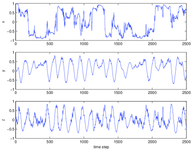
Figure 1: The evolution of one ensemble Bloch vector with $\varphi{=}0$

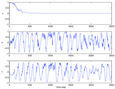
Figure 2: The evolution of one ensemble Bloch vector with $\varphi{=}\pi/2$

In contrast, measuring the quadrature with $\varphi=\pi/2$ will eventually force the atom states into the eigenstates of $\sigma_{y}$. The states are spinning around the sphere toward $z=+1$ and $z=-1$ due to the driving Hamiltonian, Fig.2, Fig.4.

The effect of imperfect measurement can be seen clearly from these results. The Bloch vectors are not confined to the surface of the unit sphere, thus the system is in mixed states. This shows that the imperfect measurements can cause loss of information about the quantum system, but nevertheless the information is consistent with the perfect case (Wiseman and Milburn, 1993c, section III.C).

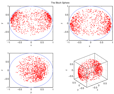
Figure 3: The steady state point of 1000 ensembles Bloch vector on the Bloch sphere with $\varphi{=}0$

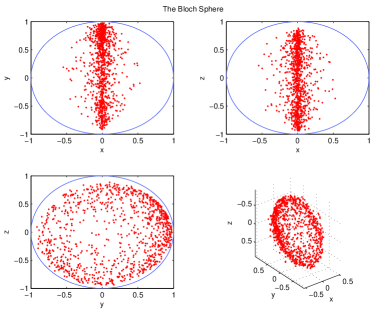
Figure 4: The steady state point of 1000 ensembles Bloch vector on the Bloch sphere with $\varphi{=}\pi/2$

IV Jump Case

To derive a pathwise solution for the jump SME (10), we choose (see for example Malcolm et al. (1999))

$$A_{t}=C^{-N_{t}},$$ (48)

and again define an unnormalized state $r_{t}$ by

$$r_{t}=A_{t}\widetilde{\rho}_{t}A^{\dagger}_{t},$$ (49)

where $\widetilde{\rho}_{t}$ is a solution of the unnormalized jump stochastic master equation (15). Then $r_{t}$ solves the pathwise master equation

$$\dot{r_{t}}=-A_{t}GA^{-1}_{t}r_{t}-r_{t}(A^{\dagger}_{t})^{-1}G^{\dagger}A^{\dagger}_{t}+(1-\eta)\lambda\mathcal{J}\!r_{t}+\eta\lambda r_{t}.$$ (50)

Moreover, solutions $\rho_{t}$, $\widetilde{\rho}_{t}$ to the stochastic master equations (10), (15) can be obtained from a solution $r_{t}$ to (50) via the formulas

$$\widetilde{\rho}_{t}=A^{-1}_{t}r_{t}(A^{\dagger}_{t})^{-1},\ \ \rho_{t}=\frac{A^{-1}_{t}r_{t}(A^{\dagger}_{t})^{-1}}{{\rm tr}[A^{-1}_{t}r_{t}(A^{\dagger}_{t})^{-1}]}.$$ (51)

In the case of perfect measurement and initial pure states, the jump SME (50) admits the jump pathwise Schrodinger equation

$$\dot{|\phi_{t}\rangle}=\left(-A_{t}GA_{t}^{-1}+\frac{\lambda}{2}I\right)|\phi_{t}\rangle.$$ (52)

The pathwise solutions (50) and (52) appear as ordinary equation without stochastic integrals in terms of $dN_{t}$; the counting observation result $N_{t}$ enters as a parameter in $A_{t}$. These solutions are also defined for all continuous counting observation paths.

However, we note that for the case of the jump SME, the pathwise solution might not be so useful for computation, and existing techniques (see, e.g. (Gardiner and Zoller, 2000, Chapters 11)) may be preferable.

V Conclusion

In this paper we have proposed the pathwise reformulation of the stochastic master equations for two cases; quantum diffusion and jump. These reformulations provide solution that is defined for all measurement paths and enjoy continuity properties. These robustness characteristic would be useful when applied to quantum filtering problem such as in quantum feedback control.

The results we have established are valid for scalar measurements, but can easily be generalized to the case of multiple measurements provided the interaction operators commute. It is not known if the results generalize in case the interaction operators do not commute.

Appendix A Proof of Pathwise Equations

In this appendix we prove the assertions of sections III.1 and IV concerning the pathwise equations.

We first consider the diffusion case and verify (19) and (20). The calculations are simple but needs frequent and careful use of Ito’s rule. Differentiate (18),

$$dr_{t} = dA_{t}.\widetilde{\rho}_{t}A_{t}^{\dagger}+A_{t}d\widetilde{\rho}_{t}.A_{t}^{\dagger}+A_{t}\widetilde{\rho}_{t}.dA_{t}^{\dagger}+A_{t}d\widetilde{\rho}_{t}.dA_{t}^{\dagger}$$ (53)

$$+\>dA_{t}.\widetilde{\rho}_{t}.dA_{t}^{\dagger}+dA_{t}.d\widetilde{\rho}_{t}.A_{t}^{\dagger}+dA_{t}.d\widetilde{\rho}_{t}.dA_{t}^{\dagger},$$

and (17),

$$dA_{t} = \displaystyle\frac{\partial A_{t}}{\partial y_{t}}dy_{t}+\frac{\partial A_{t}}{\partial t}dt+\frac{1}{2}\frac{\partial^{2}A_{t}}{\partial y_{t}^{2}}\,dy_{t}^{2}$$ (54)

$$= -A_{t}\frac{L}{\kappa^{2}}dy_{t}+A_{t}\frac{L^{2}}{2\kappa^{2}}dt+\frac{1}{2}(\frac{-L}{\kappa^{2}})(-A_{t}\frac{L}{\kappa^{2}})\kappa^{2}dt$$

$$= -A_{t}\frac{L}{\kappa^{2}}dy_{t}+A_{t}\frac{L^{2}}{\kappa^{2}}dt.$$

Similarly,

$$dA_{t}^{\dagger}=-A_{t}^{\dagger}\frac{L^{\dagger}}{\kappa^{2}}dy_{t}+A_{t}^{\dagger}\frac{(L^{\dagger})^{2}}{\kappa^{2}}dt.$$ (55)

Put (9), (54), (55) together into (53), and carefully using Ito’s rule, we obtain (19).

In the jump case we prove (50) and (51) analogously to the diffusion case. We need to use Ito’s rule for $dN_{t}$, i.e. $dN_{t}^{2}=dN_{t}$ and $dN_{t}dt=0$. Any higher order of differential involving $dt$ is zero. Differentiate (49),

$$dr_{t} = dA_{t}.\widetilde{\rho}_{t}A_{t}^{\dagger}+A_{t}d\widetilde{\rho}_{t}.A_{t}^{\dagger}+A_{t}\widetilde{\rho}_{t}.dA_{t}^{\dagger}+A_{t}d\widetilde{\rho}_{t}.dA_{t}^{\dagger}$$ (56)

$$+dA_{t}.\widetilde{\rho}_{t}.dA_{t}^{\dagger}+dA_{t}.d\widetilde{\rho}_{t}.A_{t}^{\dagger}+dA_{t}.d\widetilde{\rho}_{t}.dA_{t}^{\dagger},$$

and (17),

$$dA_{t} = A_{t}\left(\displaystyle\sum_{n=1}^{\infty}(-1)^{n}\frac{(\ln C)^{n}}{n!}\right)\,dN_{t}$$ (57)

$$= A_{t}(C^{-1}-I)\,dN_{t}.$$

The infinite series arise due to the Ito’s rule that higher orders of $dN_{t}$ do not vanish. Similarly,

$$dA_{t}^{\dagger}=A_{t}^{\dagger}((C^{\dagger})^{-1}-I)\,dN_{t}$$ (58)

Put (15), (57), (58) together into (56), and carefully using Ito’s rule, we obtain (50).

Appendix B Continuity Proof

We provide the proof of the continuity result (21) of section III.1.

In view of (20), it is enough to verify that

$$\parallel r^{1}-r^{2}\parallel_{T}\leq C\parallel y^{1}-y^{2}\parallel_{T}.$$ (59)

Let Equation (19) defined for all $t\in[0,T]$, and we rewrite it in term of matrices $\mathcal{R}_{t}=\mathcal{R}(y_{t})$ and $\mathcal{M}$ such that

$$\dot{r_{t}}=\mathcal{R}_{t}r_{t}+r_{t}\mathcal{R}^{\dagger}_{t}+\mathcal{M}(r_{t}).$$ (60)

Given observation records $y_{t}^{1}$, $y_{t}^{2}$ we have the corresponding pathwise solutions $r_{t}^{1}=r_{t}(y_{t}^{1})$, $r_{t}^{2}=r_{t}(y_{t}^{2})$ and matrices $\mathcal{R}_{t}^{1}=\mathcal{R}(y_{t}^{1})$, $\mathcal{R}_{t}^{2}=\mathcal{R}(y_{t}^{2})$.

It follows

$$|r_{t}^{1}-r_{t}^{2}| \leq \displaystyle\int_{0}^{t}\left|\mathcal{R}_{s}^{1}r_{s}^{1}-\mathcal{R}_{s}^{2}r_{s}^{2}+r_{s}^{1}\mathcal{R}_{s}^{1{\dagger}}-r_{s}^{2}\mathcal{R}_{s}^{2{\dagger}}\right.$$

$$+\left.\mathcal{M}(r_{s}^{1})-\mathcal{M}(r_{s}^{2})\right|ds$$

$$\leq \displaystyle\int_{0}^{t}\left|\mathcal{R}_{s}^{1}r_{s}^{1}-\mathcal{R}_{s}^{2}r_{s}^{1}+\mathcal{R}_{s}^{2}r_{s}^{1}-\mathcal{R}_{s}^{2}r_{s}^{2}\right.$$

$$+r_{s}^{1}\mathcal{R}_{s}^{1{\dagger}}-r_{s}^{1}\mathcal{R}_{s}^{2{\dagger}}+r_{s}^{1}\mathcal{R}_{s}^{2{\dagger}}-r_{s}^{2}\mathcal{R}_{s}^{2{\dagger}}$$

$$\left.\!+\mathcal{M}(r_{s}^{1})-\mathcal{M}(r_{s}^{2})\right|ds$$

$$\leq \displaystyle\int_{0}^{t}\left\{\left|\mathcal{R}_{s}^{1}-\mathcal{R}_{s}^{2}\right||r_{s}^{1}|+|r_{s}^{1}|\left|\mathcal{R}_{s}^{1{\dagger}}-\mathcal{R}_{s}^{2{\dagger}}\right|\right\}ds$$

$$+\displaystyle\int_{0}^{t}\left\{\left|\mathcal{R}_{s}^{2}\right||r_{s}^{1}-r_{s}^{2}|+|r_{s}^{1}-r_{s}^{2}|\left|\mathcal{R}_{s}^{2{\dagger}}\right|\right\}ds$$

$$+\displaystyle\int_{0}^{t}\left\{\left|\mathcal{M}(r_{s}^{1})-\mathcal{M}(r_{s}^{2})\right|\right\}ds$$

$$\leq C_{1}\parallel y^{1}-y^{2}\parallel_{T}+\displaystyle\int_{0}^{t}C_{2}|r_{s}^{1}-r_{s}^{2}|ds$$

Here $C_{1}$ and $C_{2}$ depend on $\parallel y^{1}\parallel_{T}$, $\parallel y^{2}\parallel_{T}$ and $T$. By Gronwall’s lemma, we have

$$|r_{t}^{1}-r_{t}^{2}| \leq C_{1}\parallel y^{1}-y^{2}\parallel_{T}\exp\left\{\displaystyle\int_{0}^{t}C_{2}ds\right\}$$

$$\leq C\,\parallel y^{1}-y^{2}\parallel_{T}$$

for all $0\leq t\leq T$, which implies (59) as required.

References

- Gardiner and Zoller (2000) C. Gardiner and P. Zoller, Quantum Noise (Springer, Berlin, 2000).
- Carmichael (1993) H. Carmichael, An Open Systems Approach to Quantum Optics (Springer, Berlin, 1993).
- Wiseman and Milburn (1993a) H. Wiseman and G. Milburn, Phys. Rev. A 47, 642 (1993a).
- Barchielli and Belavkin (1991) A. Barchielli and V. Belavkin, J. Phys. A: Math. Gen. 24, 1495 (1991).
- Belavkin (1992) V. Belavkin, Commun. Math. Phys. 146, 611 (1992).
- Gardiner (2004) C. Gardiner, Handbook of Stochastic Methods for Physics, Chemistry and the Natural Sciences (Springer, Berlin, 2004), 3rd ed.
- Karatzas and Shreve (1988) I. Karatzas and S. Shreve, Brownian Motion and Stochastic Calculus (Springer, New York, 1988).
- Kloeden and Platen (1992) P. Kloeden and E. Platen, Numerical Solution of Stochastic Differential Equations (Springer, New York, 1992).
- Clark (1978) J. M. C. Clark, in Communication System and Random Processes Theory, edited by J. Skwirzynski, NATO Advanced Studies Institute Series (Sijthoff and Noordhoff, Alphen aan den Rijn, 1978), pp. 721–734.
- Elliott (1982) R. Elliott, Stochastic Calculus and Applications (Springer Verlag, New York, 1982).
- Wong and Hajek (1985) E. Wong and B. Hajek, Stochastic Processes in Engineering Systems (Springer Verlag, New York, 1985).
- Davis (1979) M. H. A. Davis, in Proceeding of the 18th IEEE Conference on Decision and Control pp. 176–180 (1979).
- Sussmann (1978) H. Sussmann, The Annals of Probability 6, 19 (1978).
- (14) I. Kurniawan and M. R. James, eprint To appear, 43rd IEEE Conference on Decision and Control, December, 2004.
- Nielsen and Chuang (2000) M. Nielsen and I. Chuang, Quantum Computation and Quantum Information (Cambridge University Press, Cambridge, 2000).
- Merzbacher (1998) E. Merzbacher, Quantum Mechanics (Wiley, New York, 1998), 3rd ed.
- Wiseman and Milburn (1994) H. Wiseman and G. Milburn, Phys. Rev. A 49, 1350 (1994).
- Caves and Milburn (1987) C. Caves and G. Milburn, Phys. Rev. A 36, 5543 (1987).
- Milburn (1996) G. Milburn, Quantum Technology, Frontiers of Science (Allen & Unwin, St. Leonards, Australia, 1996).
- Belavkin (2001) V. Belavkin, Progress in Quantum Electronics 25, 3 (2001).
- Wiseman and Milburn (1993b) H. Wiseman and G. Milburn, Phys. Rev. Lett. 70, 548 (1993b).
- Wiseman and Milburn (1993c) H. Wiseman and G. Milburn, Phys. Rev. A 47, 1652 (1993c).
- Bachor (1998) H. Bachor, A Guide to Experiments in Quantum Optics (Wiley-VCH, Weinheim, Germany, 1998).
- Malcolm et al. (1999) W. P. Malcolm, R. J. Elliott, and M. R. James, in Proceeding of the 38th IEEE Conference on Decision and Control pp. 143–150 (1999).