Spontaneous emission of a photon: wave packet structures and atom-photon entanglement

Abstract

Spontaneous emission of a photon by an atom is described theoretically in three dimensions with the initial wave function of a finite-mass atom taken in the form of a finite-size wave packet. Recoil and wave-packet spreading are taken into account. The total atom-photon wave function is found in the momentum and coordinate representations as the solution of an initial-value problem. The atom-photon entanglement arising in such a process is shown to be closely related to the structure of atom and photon wave packets which can be measured in the coincidence and single-particle schemes of measurements. Two predicted effects, arising under the conditions of high entanglement, are anomalous narrowing of the coincidence wave packets and, under different conditions, anomalous broadening of the single-particle wave packets. Fundamental symmetry relations between the photon and atom single-particle and coincidence wave packet widths are established. The relationship with the famous scenario of Einstein-Podolsky-Rosen is discussed.

I Introduction

Beginning with the famous original derivation of natural linewidth by Weisskopf and Wigner WW , spontaneous emission of atoms has been considered traditionally, explicitly or not, in the approximations of an infinitely heavy atom and an infinitely narrow center-of-mass wave function. Rigorously, neither of these approximations is ever correct. In a more realistic formulation, for a finite-mass atom and a finite-size center-of-mass atomic wave function, the problem of spontaneous emission was considered by Rza̧żewski and Żakowicz RzaZak . Chan et al. JHE showed that such a formulation gives rise to questions about photon-atom entanglement after emission. They investigated this in one space dimension in the frame of Schmidt mode analysis JHE ; JHE1 ; Kazik . Atomic and photon position-dependent Schmidt eigenfunctions were found numerically and the conditions under which entanglement is large were determined.

In this work we continue investigation of this problem. Its solution is a bridge between two quite different regimes of two-particle entanglement. These two regimes are both concerned with entanglement arising from the breakup of a composite object into two “fragments” that are free to move away from the breakup point, and in the ideal case are constrained only by momentum and energy conservation. One regime deals with zero-mass particles (two photons), and here the most common context is spontaneous parametric down-conversion Huang-Eberly93 ; Rubin ; Monken-etal ; BostonGrp ; Barbosa ; Law-etal00 ; Law-Eberly04 ; Kulik . The second regime treats two finite-mass fragments: electron and ion in photoionization PRA , two atoms in molecular dissociation Opatrny-etal03 ; PRA ; Opatrny-etal04 ; LANL , or even electron and positron in pair production Krekora-etal . Two-particle scattering provides another view of breakup entanglement Grobe-etal94 ; Law04 ; Mishima-etal04 . The regime where one fragment is a photon and the other is massive raises issues that deserve separate attention.

In contrast to the approach taken in Refs. JHE ; JHE1 ; Kazik , we consider this bridging regime in a more realistic 3D picture. We obtain the entangled position-dependent atom-photon wave function as the solution of an initial-value problem. Atomic recoil is taken into account and the initial atomic wave function is taken in the form of a finite-size wave packet. We investigate the structure of the photon and atomic wave packets that arise after emission of a photon. In analogy with our treatment of entanglement in photoionization and photodissociation PRA , we focus on experimentally accessible quantities. We introduce the parameter $R$ given by the ratio of the positional wave packet widths to be measured singly or in coincidence, thus incorporating both conditioned and unconditioned schemes of registration. Spreading of the atomic wave packet is shown to play a crucial role for the time evolution of the ratio $R$. Two specific predicted effects are entanglement-induced narrowing of the coincidence-scheme photon wave packet and, under different conditions, a large broadening of the photon wave packet to be found from the single-particle measurements. We note that coincidence or conditional detection in regard to entanglement was first carefully examined by Reid Reid in the context of photonic squeezed states. In that case one can define artificial position and momentum variables using the photonic $\hat{a}$ and $\hat{a}^{\dagger}$ operators, but there is not a simple analog of wave packet spreading, which is our focus here.

In the next Section the general problem of the position-dependent photon wave function is briefly discussed. In Section III we outline the solution of the problem of spontaneous emission from a finite-mass atom, characterized by a finite-size center-of-mass wave packet. In Section IV we formulate a series of approximations that are used to find an explicit expression for the photon-atom wave function in the coordinate representation, and in section V its entanglement features are analyzed. In Section VI we investigate the wave packet structure in the coordinate representation. In Section VII we introduce the main parameter $R$ and show that $R\gg 1$ characterizes the regions where an anomalously narrow or wide wave packet can be found. Wave packets in the momentum representation are analyzed in Section VIII, and a series of symmetry relations between the wave packet widths is derived. In Section IX we establish uncertainty relations following from the high entanglement condition. One of them is the coincidence uncertainty relation which is shown to restrict the products of the particle’s coordinate and momentum uncertainties to be less than one (or $\hbar$). The relationship with the famous Einstein-Podolsky-Rosen scenario EPR is described. Experimental aspects are discussed briefly in Section X.

II Position-dependent photon wave function

Although one can find examples AB ; LL of a very strongly formulated opinion that the position-dependent photon wave function does not exist, in quantum optics the photon wave function is accepted rather widely MW ; SZ ; ON . To outline the way in which this concept can be introduced, let us consider the state vector for the electromagnetic field, given by an arbitrary superposition of one-photon states $\mid 1_{\vec{k}\lambda}\rangle$ with definite values of the wave vector $\vec{k}$ and polarization $\lambda$

$$|\Psi^{EM}(t)\rangle=\sum_{\vec{k}\lambda}C_{\vec{k}\lambda}\,e^{-i\omega_{k}t}\mid 1_{\vec{k}\lambda}\rangle\,,$$ (1)

where $\omega_{k}=c|\vec{k}|$, $k_{\alpha}=n_{\alpha}2\pi/L$ with $\alpha=x,y,z$; $L$ is the normalization length, and $\lambda=1,2$ is the polarization state of the photon. The state vector (1) is conveniently normalized:

$$\langle\Psi^{EM}(t)\mid\Psi^{EM}(t)\rangle=\sum_{\vec{k}\lambda}\mid C_{\vec{k}\lambda}\mid^{\,2}\,\equiv\sum_{\lambda}\int d\vec{k}\,\mid\widetilde{C}_{\vec{k}\lambda}\mid^{\,2}\,=1,$$ (2)

where $\widetilde{C}_{\vec{k}\lambda}=(L/2\pi)^{3/2}\,C_{\vec{k}\lambda}$. Here and below we use in parallel both discrete and continuous sets of wave vectors (in the normalization box $L^{3}$ and in free space, respectively) with the sums and integrals over wave vectors transformed from one to the other with the help of the relation $\sum_{\vec{k}}=\frac{L^{3}}{(2\pi)^{3}}\int d\vec{k}$.

The expansion coefficients $C_{\vec{k}\lambda}$ in the superposition (1) are interpreted naturally as the photon wave function in the momentum representation. The probability density to find (register) a photon with a momentum around $\hbar\vec{k}$ is given by

$$\frac{dw}{d(\hbar\vec{k})}=\frac{1}{\hbar^{3}}\sum_{\lambda}\left|\,\widetilde{C}_{\vec{k}\lambda}\right|^{\,2}.$$ (3)

In quantum electrodynamics the operators of the field vector potential and electric field-strength are given by

$$\hat{\vec{\mathcal{A}}}(\vec{r})=\sum_{\vec{k}\lambda}\sqrt{\frac{2\pi\hbar c^{2}}{\omega_{k}\,L^{3}}}\,\left\{\vec{e}_{\vec{k}\,\lambda}\,e^{i\vec{k}\cdot\vec{r}}\,\hat{a}_{\vec{k}\lambda}+\vec{e}_{\vec{k}\,\lambda}^{\;*}\,e^{-i\vec{k}\cdot\vec{r}}\,\hat{a}_{\vec{k}\lambda}^{{\dagger}}\right\}$$ (4)

and

$$\hat{\vec{\mathcal{E}}}^{\,}(\vec{r}^{\,})=i\sum_{\vec{k}\lambda}\sqrt{\frac{2\pi\hbar\omega_{k}}{L^{3}}}\,\left\{\vec{e}_{\vec{k}\,\lambda}\,e^{i\vec{k}\cdot\vec{r}}\,\hat{a}_{\vec{k}\lambda}-\vec{e}_{\vec{k}\,\lambda}^{\;*}\,e^{-i\vec{k}\cdot\vec{r}}\,\hat{a}_{\vec{k}\lambda}^{{\dagger}}\right\}\,,$$ (5)

where $\hat{a}_{\vec{k}\lambda}$ and $\hat{a}_{\vec{k}\lambda}^{{\dagger}}$ are the photon annihilation and creation operators and ${\vec{e}}_{\vec{k}\,\lambda}$ are the polarization vectors, ${\vec{e}}_{\vec{k}\,\lambda}\perp\vec{k}$. The position-dependent density of the field energy is defined as

$$\frac{dE_{f}(\vec{r},t)}{d\vec{r}} = \frac{1}{4\pi}\;\langle\Psi(t)|\hat{\vec{\mathcal{E}}}^{\,{\dagger}}(\vec{r})\cdot\hat{\vec{\mathcal{E}}}(\vec{r})|\Psi(t)\rangle$$ (6)

$$= \frac{1}{L^{3}}\left|\sum_{\vec{k}\lambda}\sqrt{\hbar\omega_{k}}\;\vec{e}_{\vec{k}\,\lambda}\,C_{\vec{k}\lambda}\,e^{i(\vec{k}\cdot\vec{r}-\omega_{k}t)}\right|^{2}.$$

The total field energy of the state (1) is given by the integrated density of energy of Eq. (6)

$$E_{f}=\sum_{\vec{k}\lambda}\hbar\omega_{k}\,\left|\,C_{\vec{k}\lambda}\right|^{\,2}=\sum_{\lambda}\int d\vec{k}\;\hbar\omega_{k}\,\left|\,\widetilde{C}_{\vec{k}\lambda}\right|^{\,2}\equiv\hbar\overline{\omega},$$ (7)

where, by definition, $\overline{\omega}$ is the mean photon frequency of the superposition (1).

In general the position-dependent density of the field energy $dE_{f}/d{\vec{r}}$ can also be presented in the form

$$\frac{dE_{f}(\vec{r},t)}{d\vec{r}}=\hbar\overline{\omega}\left|{\vec{\Psi}}_{ph}({\vec{r}},t)\right|^{2},$$ (8)

where, following the Mandel-Wolf definition MW , ${\vec{\Psi}}_{ph}({\vec{r}},t)$ is the vectorial position-dependent one-photon photon wave function

$${\vec{\Psi}}_{ph}({\vec{r}},t) = \frac{1}{L^{3/2}\sqrt{\overline{\omega}}}\sum_{\vec{k}\lambda}\sqrt{\omega_{k}}\;\vec{e}_{\vec{k}\,\lambda}\;C_{\vec{k}\lambda}\,e^{i(\vec{k}\cdot\vec{r}-\omega_{k}t)}$$ (9)

$$= \frac{1}{(2\pi)^{3/2}\sqrt{\overline{\omega}}}\sum_{\lambda}\int d{\vec{k}}\,\sqrt{\omega_{k}}\;\vec{e}_{\vec{k}\lambda}\;\widetilde{C}_{\vec{k}\lambda}e^{i(\vec{k}\cdot\vec{r}-\omega_{k}t)}.$$

Owing to Eq. (7), the vectorial photon wave function (9) is also normalized:

$$\int d\vec{r}\;\left|\vec{\Psi}_{ph}(\vec{r},t)\right|^{2}=1.$$ (10)

It should be noted that the interpretation of $\vec{\Psi}_{ph}({\vec{r}},t)$ of Eq. (9) as the position-dependent photon wave function is only partially satisfactory. By definition, this interpretation is good for the calculation of the average photon energy or frequency $\overline{\omega}$. But if we try to calculate with the help of $\vec{\Psi}_{ph}({\vec{r}},t)$ the average values of other quantities, e.g., the average photon momentum $\hbar\overline{{\vec{k}}}$, in general the result will be wrong because of the factor $\sqrt{\omega_{k}}$ in Eq. (9). However, there is a class of states for which this problem does not arise and the definition of the photon wave function is non-controversial. This is the case of narrow-band superpositions, for which the coefficients $C_{\vec{k}\lambda}$ in (1) are substantially non-zero only inside a narrow spectral range $\Delta\omega$

$$|\,\omega_{k}-\overline{\omega}\,|\sim\Delta\omega\ll\overline{\omega}.$$ (11)

In this case the factor $\sqrt{\omega_{k}}$ on the right-hand side of Eq. (9) can be approximated by $\sqrt{\overline{\omega}}$ to give simpler expressions for the photon wave function

$$\vec{\Psi}_{ph}(\vec{r},t) = \frac{1}{L^{3/2}}\sum_{\vec{k}\lambda}\,C_{\vec{k}\lambda}\,\vec{e}_{\vec{k}\,\lambda}\,e^{i(\vec{k}\cdot\vec{r}-\omega_{k}t)}$$ (12)

$$= \frac{1}{(2\pi)^{3/2}}\int d\vec{k}\sum_{\lambda}\,\widetilde{C}_{\vec{k}\lambda}\,\vec{e}_{\vec{k}\,\lambda}\,e^{i(\vec{k}\cdot\vec{r}-\omega_{k}t)}.$$

In the case of spontaneous decay of atomic levels the spectral width of the emitted light $\Delta\omega$ is the same as the decay rate $\gamma$, which is always much less than the mean emitted frequency $\overline{\omega}$. So, for spontaneously emitted photon states the inequality (11) is always satisfied and the photon wave packet spectral width is relatively small. The Fourier transform (12) of the photon momentum wave function establishes then an effective photon wave packet width $c/\gamma$ in coordinate space.

Note that in speaking about the position-dependent photon wave function $\vec{\Psi}_{ph}(\vec{r},t)$ we assume that its squared absolute value determines the probability density of the photon registration by a detector located at the point $\vec{r}$. Although below we will use the concept of the photon position vector $\vec{r}_{ph}$, we will keep in mind that in fact this is the position of the photon detector.

III Spontaneous emission

To specify the problem to be considered, let us assume that initially an atom is prepared in a pure excited $P$-state with zero projection of its angular momentum upon the $z$-axis. The preparation can be done, for example, with the help of excitation from the ground $S$-state by a resonant laser $\pi$-pulse with the linear polarization vector $\vec{e}_{0}$ along the $z$ axis. If the pulse duration of the exciting pulse is short compared to the life-time of the excited level, for spontaneous emission the process of excitation is practically instantaneous, and this reduces the problem of spontaneous emission to a solution of an initial-value problem with a suddenly turned-on interaction.

Let the spontaneous emission of a photon arise from the atomic transition back to the same ground state $|g\rangle$ from which the atom was initially excited. Then, in the long-time limit $t\gg 1/\gamma$, where $\gamma$ is the decay rate, all the atomic population returns to the ground state, and the two-particle atom-photon state vector takes the form

$$|\,\Psi\rangle=\sum_{\vec{q},\,\vec{k}}C_{\vec{q},\,\vec{k}\,}(t)\exp\left\{-i\left(\frac{q^{2}}{2M}+E_{g}+\omega_{k}\right)t\right\}\,|\,g\rangle|\;\vec{q}\;\rangle|\,1_{\vec{k}\,}\rangle\,,$$ (13)

where $M$ is the total mass of the atom, $\vec{q}\,$ is its momentum, and $\vec{k}$ is the photon wave vector in a one-photon state $|\,1_{\vec{k}\,}\rangle$. Now and henceforth in this paper we use a system of units with $\hbar=1$ and do not make any difference between momenta and wave vectors of particles or fields.

Multiplied by $(L/2\pi)^{3}$, the expansion coefficient $C_{\vec{q},\,\vec{k}\,}(t)$ can be considered as the atom-photon momentum-space wave function. It describes an entangled atom-photon state when it is not factorable in the variables $\vec{q}$ and $\vec{k}$. Summation over photon polarizations in Eq. (13) is unnecessary because for any given $\vec{k}$ the atom can only emit a photon with the polarization vector $\vec{e}_{k}$ in the plane $\{\vec{k},\vec{e}_{0}\}$

$$\vec{e}_{k}=\frac{k^{2}\vec{e}_{0}-\vec{k}(\vec{k}\cdot\vec{e}_{0})}{k\sqrt{k^{2}-(\vec{k}\cdot\vec{e}_{0})^{2}}}\;.$$ (14)

The coefficients $C_{\vec{q},\,\vec{k}\,}(t)$ can be found in Weisskopf-Wigner approximation to be given by RzaZak

$$C^{(W-W)}_{\vec{q},\,\vec{k}\,}(t)\Big{|}_{\gamma t\gg 1}=-\frac{ie\,z_{eg}\,\omega_{0}\sqrt{2\pi}}{L^{3/2}\sqrt{\omega_{k}}}\,\frac{B(\vec{q}+\vec{k})\,\sin\vartheta_{k}}{\displaystyle\frac{q^{2}-(\vec{q}+\vec{k}\,)^{2}}{2M}+\omega_{k}-\omega_{0}+i\frac{\gamma}{2}}\,,$$ (15)

where $z$ is the intra-atomic electron $z$-coordinate, $z_{eg}$ is the matrix element of excited-ground state transition, and $\vartheta_{k}$ is the angle between $\vec{k}$ and the intra-atomic electron $z$-axis. The function $B(\vec{q})$ in Eq. (15) is the initial atomic wave function in the momentum (wave vector) representation taken below in the Gaussian form

$$B(\vec{q})=\left(\frac{2\pi}{L}\frac{a_{0}}{\sqrt{\pi}}\right)^{3/2}\exp\left(-\frac{a_{0}^{2}\,q^{2}}{2}\right),$$ (16)

so the corresponding initial atomic center-of-mass wave function in the coordinate representation has a Gaussian form too

$$\Psi_{at}(\vec{r}_{at},\,t=0)=\frac{1}{L^{3/2}}\sum_{\vec{q}}B(\vec{q})e^{i\vec{q}\cdot\vec{r}_{at}}=\left(\frac{1}{\sqrt{\pi}a_{0}}\right)^{3/2}\exp\left(-\frac{r_{at}^{2}}{2a_{0}^{2}}\right).$$ (17)

where $a_{0}$ is here not the Bohr radius but the initial size of the atomic wave packet. Such a state of the center-of-mass motion can be created, for example with the help of a trap. We assume that at the same time $t=0$ when the trapped atom is excited and spontaneous emission begins, the field of the trap is switched off, and free spreading of the atomic center-of-mass wave packet begins.

IV The atom-photon wave function

In analogy with the definition of the photon wave function in Eq. (9), the position-dependent two-particle atom-photon vectorial wave function can be defined as

$$\vec{\Psi}(\vec{r}_{at},\vec{r}_{ph},t)=\frac{1}{L^{3}}\sum_{\vec{q},\,\vec{k}}C_{\vec{q},\,\vec{k}\,}(t)\,\vec{e}_{k}\,\exp\left\{i\left(\vec{q}\cdot\vec{r}_{at}+\vec{k}\cdot\vec{r}_{ph}\right)\right\}\,\exp\left\{-i\left(\frac{q^{2}}{2M}+E_{g}+\omega_{k}\right)t\right\},$$ (18)

where $\vec{r}_{at}$ and $\vec{r}_{ph}$ are, correspondingly, the atomic center-of-mass and photon position vectors, and $\vec{e}_{k}$ is given by Eq. (14). In accordance with the concluding remark of Section II, the terms of the $``\text{position vectors}"$ are used conventionally. Rigorously, the interpretation of the two-particle atom-photon wave function is based on the assumption that its squared absolute value determines the probability density of registering atoms and photons by the corresponding detectors located at the points $\vec{r}_{at}$ and $\vec{r}_{ph}$.

With $C_{\vec{q},\,\vec{k}\,}(t)$ and $B(\vec{q})$ taken from Eqs. (15) and (16) and with the integration variable $\vec{q}$ replaced by $\vec{q}-\vec{k}$ we can reduce Eq. (18) to the form

$$\vec{\Psi}(\vec{r}_{at},\vec{r}_{ph},t) = -\displaystyle\frac{i\,e\,z_{eg}\,\omega_{0}a_{0}^{3/2}\,e^{-iE_{g}t}}{(2\pi)^{4}\pi^{3/4}\sqrt{c}}\int d\vec{q}\,\exp\left[-\frac{q^{2}}{2}\left(a_{0}^{2}+\frac{it}{M}\right)+i\,\vec{q}\cdot\vec{r}_{at}\right]$$ (19)

$$\times\displaystyle\int_{0}^{\infty}k^{3/2}\,dk\,\exp\left(-\,\frac{it}{2M}\,k^{2}\,\right)\int d\Omega_{k}\,\vec{e}_{k}\;\sin\vartheta_{k}\;\displaystyle\frac{\exp\left(i\,(\vec{k}\cdot\vec{\rho}-ckt)+\,\displaystyle\frac{it}{M}\,\vec{q}\cdot\vec{k}\,\right)}{-\displaystyle\frac{\vec{q}\cdot\vec{k}}{M}+\frac{k^{2}}{2M}+\omega_{k}-\omega_{0}+i\frac{\gamma}{2}},\ \$$

where $\vec{\rho}=\vec{r}_{ph}-\vec{r}_{at}$ and $d\Omega_{k}$ is a solid angle element in the direction of $\vec{k}$.

Analytical calculation of these integrals can be performed only approximately. As the first approximation let us put $\left|\vec{k}\right|\approx\omega_{0}/c$ in all the terms of the integrand of Eq. (19) proportional to $k^{2}$ and $\vec{k}\cdot\vec{q}$. The precision of this approximation is determined by small parameters proportional to $\omega_{0}/Mc^{2}\ll 1$. The second key approximation can be referred to as the far zone approximation, which means that the distance $\rho$ is assumed to be large enough, i.e., $k\rho\gg 1$. The validity of this condition follows already from our original assumptions $t\gg 1/\gamma\gg 1/\omega$, which indicate immediately that at $\rho\sim ct$ we have $k\rho\sim\omega t\gg 1$. In the far-zone approximation the main contribution to the integral over $d\Omega_{k}$ is given by those $\vec{k}$ close to the direction of $\vec{\rho}$. Owing to this assumption we put $\vec{k}\|\vec{\rho}$ everywhere in the integrand of Eq. (19) except in the factor $\exp(i\vec{\rho}\cdot\vec{k})\equiv\exp(i\rho kx)$, where $x$ is the cosine of the angle between $\vec{k}$ and $\vec{\rho}$. This is the only remaining function of $x$ and it is easily integrated to give two terms, proportional to $e^{ik\rho}$ and $e^{-ik\rho}$. These two terms correspond to outgoing and incoming spherical waves and, owing to the far-zone assumption, the incoming wave gives an exponentially small contribution which can be dropped. Thus, the result after the integration over $d\Omega_{k}$ is given by

$$\vec{\Psi}(\vec{r}_{at},\vec{r}_{ph},t) = -\left[\displaystyle\frac{e\,z_{eg}\,\omega_{0}a_{0}^{3/2}\,e^{-iE_{g}t-i\omega_{0}^{2}t/2Mc^{2}}}{(2\pi)^{3}\pi^{3/4}\sqrt{c}}\right]\displaystyle\frac{\vec{e}_{\rho}^{\,\perp}\,\sin\vartheta_{\rho}}{\rho}$$ (20)

$$\times\displaystyle\int d\vec{q}\;\exp\left[-\frac{q^{2}}{2}\left(a_{0}^{2}+\frac{it}{M}\right)+i\,\vec{q}\cdot\vec{r}_{at}+\displaystyle\frac{it}{M}\,\frac{q_{\rho}\,\omega_{0}}{c}\,\right]\;$$

$$\times\displaystyle\int_{0}^{\infty}dk\;\displaystyle\frac{k^{1/2}\;\exp\left[i\,k(\rho-ct)\right]}{-\displaystyle\frac{q_{\rho}\,\omega_{0}}{Mc}+\frac{\omega_{0}^{2}}{2Mc^{2}}+\omega_{k}-\omega_{0}+i\frac{\gamma}{2}},$$

where $\vec{e}_{\rho}^{\,\perp}$ is the unit vector perpendicular to $\vec{\rho}$ and lying on the plane $\{\vec{e}_{0},\,\vec{\rho\,}\}$, $\vartheta_{\rho}$ is the angle between $\vec{e}_{0}$ and $\vec{\rho}$, and $q_{\rho}$ is the projection of the vector $\vec{q}$ on the direction of $\vec{\rho}$.

Now, in accordance with the spirit of the Weisskopf-Wigner approximation, the integral over $k$ is calculated by the residue method with the lower limit of integration extended to $-\infty$ and the integrand continued analytically into the complex plane $k$. Then we get

$$\vec{\Psi}(\vec{r}_{at},\vec{r}_{ph},t) \Rightarrow \displaystyle\frac{e\,z_{eg}\,\omega_{0}^{3/2}a_{0}^{3/2}}{(2\pi)^{2}\pi^{3/4}\ c^{2}}\left(\frac{\vec{e}_{\rho}^{\,\perp}\sin\vartheta_{\rho}}{\rho}\right)\,\theta(ct-\rho)\exp\left[\frac{\gamma}{2c}(\rho-ct)\right]$$ (21)

$$\times\displaystyle\int d\vec{q}\;\exp\left[-\frac{q^{2}}{2}\left(a_{0}^{2}+\frac{it}{M}\right)+i\,\vec{q}\cdot\vec{R}\right],$$

where the symbol $``\Rightarrow"$ means that all the phase factors independent of the integration variables are dropped and

$$\vec{R}\equiv\vec{r}_{at}+\frac{v_{rec}}{c}\,\vec{\rho}=\vec{r}_{at}\left(1-\frac{v_{rec}}{c}\right)+\frac{v_{rec}}{c}\,\vec{r}_{ph}.$$ (22)

Integration over $d\vec{q}\,$ in Eq. (21) can be easily performed to give the following expression for the atom-photon wave function:

$$\vec{\Psi}(\vec{r}_{at},\vec{r}_{ph},t) \Rightarrow \displaystyle\frac{e\,z_{eg}\,\omega_{0}^{3/2}}{\sqrt{2\pi}\;\pi^{3/4}\,c^{2}}\left(\frac{\vec{e}_{\rho}^{\,\perp}\sin\vartheta_{\rho}}{\rho}\right)\theta(ct-\rho)\exp\left[\frac{\gamma}{2c}(\rho-ct)\right]$$ (23)

$$\times\displaystyle\frac{1}{\left(a_{0}+it/Ma_{0}\right)^{3/2}}\,\exp\left\{-\frac{\vec{R}^{2}}{2\left(a_{0}^{2}+it/M\right)}\right\}\,,$$

where $v_{rec}=\omega_{0}/Mc$ is the atomic recoil velocity due to the emission of a photon with momentum $\omega_{0}/c$. The squared absolute joint wave function can then be written in the form

$$\left|\vec{\Psi}(\vec{r}_{at},\vec{r}_{ph},t)\right|^{\,2}=\left|\Psi_{rel}(\vec{\rho},\,t)\right|^{\,2}\times\left|\Psi_{cm}(\vec{R},\,t)\right|^{\,2}.$$ (24)

Here $\Psi_{rel}(\vec{\rho},\,t)$ is the relative motion wave function which depends only on the relative-motion position vector $\vec{\rho}=\vec{r}_{ph}-\vec{r}_{at}$. It takes the form of an entanglement-free photon wave function $\Psi_{ph}^{(0)}$ SZ

$$\left|\Psi_{rel}(\vec{\rho},\,t)\right|^{2}\equiv\left|\Psi_{ph}^{(0)}(\vec{\rho},\,t)\right|^{2}=\displaystyle\frac{3\gamma\sin^{2}\vartheta_{\rho}}{8\pi c\,\rho^{2}}\,\theta(ct-|\vec{\rho}|)\,\exp\left[\frac{\gamma}{c}(|\vec{\rho}|-ct)\right].$$ (25)

On the other hand, although there is no center of mass, $\Psi_{cm}(\vec{R},\,t)$ can be recognized as an analog of the center-of-mass wave function of two massive particles in situations such as photodissociation and photoionization PRA . In the case of atom-photon decay $\Psi_{cm}(\vec{R},\,t)$ has the form of an entanglement-free spreading atomic center-of-mass wave function $\Psi_{at}^{(0)}$. Together with the initial condition given by Eq. (17), it reads

$$\left|\Psi_{cm}(\vec{R},\,t)\right|^{2}=\left|\Psi_{at}^{(0)}(\vec{R},\,t)\right|^{2}=\left(\frac{1}{\sqrt{\pi}a(t)}\right)^{3}\exp\left(-\frac{|\vec{R}|^{2}}{a^{2}(t)}\right),$$ (26)

where $a(t)$ is the time-dependent width of the spreading atomic wave packet

$$a(t)\equiv\left(a_{0}^{2}+\frac{t^{2}}{M^{2}a_{0}^{2}}\right)^{1/2}.$$ (27)

We assume here that the atomic wave packet’s spreading time $t_{spr}\sim Ma_{0}^{2}$ is much longer than the atomic decay time $\gamma^{-1}$. This is true if the initial size of the atomic wave packet is not too small: $a_{0}\gg 1/\sqrt{\gamma M}\sim 10\ \text{nm}$ for $\gamma\sim 10^{8}$ sec^-1 and $M\sim 10^{4}m_{e}$. Under this assumption the instant of time when the wave packet spreading begins can be identified with the time $t=0$, at which the atom is excited and quickly freed from the trap, and at which the spontaneous emission process begins.

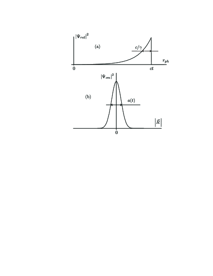
Figure 1: (a) The wave packet of a photon spontaneously emitted by an infinitely massive atom (Eq. (25)), and (b) the “center-of-mass” wave packet of a finite-mass ground-state atom (Eq. (26)).

The functions defined in Eqs. (25) and (26) are plotted in Fig. 1(a) and (b). They represent wave packets respectively for a photon spontaneously emitted by a dot-like infinitely massive atom and for a finite-mass ground-state atom with a spreading center-of-mass wave function. Note that factorization of the total wave function $\Psi$ into a product of the relative and $``\text{cm}"$ parts is a rather general feature of the decaying bipartite systems. It has been found to occur in the treatment of photoionization and photodissociation PRA as well as, in a wider sense, in spontaneous parametric down-conversion Monken-etal ; Law-etal00 ; Law-Eberly04 ; Kulik . The product of the functions shown in Fig. 1 represents the total wave function of Eq.  (23), and in Fig. 2 we show a one-dimensional analog as a density plot.

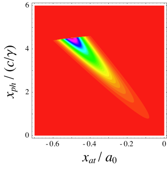
Figure 2: (Color online) The density plot of the one-dimensional analog of the total squared two-particle atom-photon wave function in Eq. (24) in the upper-left quadrant. Here $x_{at}$ and $x_{ph}$ denote the one-dimensional atom and photon coordinates. Parameters used are $\gamma t=5,v_{rel}/c=0.1$, and $ca_{0}/\gamma=0.05$.

As it should be, the total atom-photon wave packet given by Eq. (24) is appropriately normalized:

$$\int d\vec{r}_{at}\int d\vec{r}_{ph}\;\left|\vec{\Psi}(\vec{r}_{at},\vec{r}_{ph},t)\right|^{\,2}\equiv\int d\vec{R}\int d\vec{\rho}\;\left|\vec{\Psi}(\vec{R},\vec{\rho},t)\right|^{\,2}=1\,.$$ (28)

V Entanglement

As seen from Eqs. (23) and (24), the atom-photon wave packet has the form of a product of two $``\text{proto-packets}"$ given by Eqs. (25) and (26), related in this case to the wave packets of a photon and an atom considered as independent particles. However, the arguments of these proto-packets in the product in Eq. (24) are modified, or entangled, compared to those of the independent single-particle wave packets of Eqs. (25) and (26). Each of the packets $\left|\Psi_{rel}\right|^{\,2}$ and $\left|\Psi_{cm}\right|^{\,2}$ in Eq. (24) depends on both variables $\vec{r}_{at}$ and $\vec{r}_{ph}$, so that in these variables the total wave function $\vec{\Psi}(\vec{r}_{ph},\vec{r}_{at},t)$ does not factorize. This is the reason for, and clear indication of, entanglement. It should be emphasized that the conditions for obtaining atom-photon entanglement are finite mass of the atom and finite size of its center-of-mass wave function. In the limits of $M\rightarrow\infty$ and a $\delta$-localized atomic wave function, the atom-photon wave function of Eq. (24) factorizes, meaning that there is no entanglement

$$\left|\vec{\Psi}(\vec{r}_{ph},\vec{r}_{at},t)\right|^{\,2}\rightarrow\left|\Psi_{ph}^{(0)}\left(\vec{r}_{ph},\,t\right)\right|^{\,2}\delta(\vec{r}_{at}).$$ (29)

The main features of atom-photon entanglement are very similar to those already described in photoionization and photodissociation PRA . The wave functions of fragments in these processes are given by products of the fragments’ center-of-mass and relative-motion wave functions. Each of these proto-functions depends on the position vectors of both fragments, and this is the reason for entanglement. In the case of spontaneous emission, the photon does not have a mass, and the decay product’s center of mass does not exist. Nevertheless, as shown above, it is possible to present the total atom-photon wave function in the form of a product of two proto-functions with arguments depending on both atom and photon coordinates, and this explains entanglement in atomic photoionization, molecular photodissociation, and spontaneous emission from identical positions. Moreover, in Eq. (24) the argument of $\Psi_{ph}$ equals the difference of the photon and atomic position vectors $\vec{r}_{ph}-\vec{r}_{at}$, which determines the same relative-motion coordinates as in photoionization and photodissociation.

As for the argument of $\Psi_{at}$ in Eq. (24), we point out that its form is similar to the center-of-mass position vector of massive particles, with the mass ratio substituted by the ratio of velocities $v_{rec}/c$. Indeed, in the case of photoionization the center-of-mass position vector can be written as $\vec{r}_{cm}=\vec{r}_{i}(1-m_{e}/M)+\vec{r}_{e}(m_{e}/M)$ where $\vec{r}_{i}$ and $\vec{r}_{e}$ are the ion and electron position vectors, $m_{e}$ is the electron mass, and $M$ is the total mass of the system $``{\rm electron}"$. By the substitutions $\vec{r}_{i}\rightarrow\vec{r}_{at}$, $\vec{r}_{e}\rightarrow\vec{r}_{ph}$, and $m_{e}/M\rightarrow v_{rec}/c$ this expression reduces exactly to the argument of $\Psi_{at}$ in Eq. (24). This makes the analogy between the electron-ion and atom-photon entanglement almost complete.

Actually, in some sense the ratio of velocities is a more general concept than the ratio of masses. Indeed, in the case of photoionization the mass ratio can be presented in the form $m_{e}/m_{i}=v_{i}/v_{e}$, where $v_{i}$ and $v_{e}$ are the magnitudes of the classical ion and electron velocities after the break up of an atom determined by the momentum conservation rule $m_{e}\vec{v}_{e}+m_{i}\vec{v}_{i}=0$. Moreover, many results of of this work and of Ref. PRA are valid also for the process of downconversion Law-Eberly04 (see sections VII and IX below) with the velocity ratio substituted by one, because in this case the break-up fragments are two photons, and their velocities are equal.

VI Position-dependent entangled atomic and photon wave packets

One of the main ideas being presented here and in our earlier works PRA ; Kazik is the suggestion to use coincidence and single-particle measurements of wave packets of particles arising from decaying quantum systems for the analysis of particles’ entanglement and its manifestations. By single-particle measurements we mean registration of one particle independent of the other, e.g., detection of its position regardless of the position of the other particle. With repeated observations of this kind, one can reconstruct the single-particle wave packet of the chosen particle. As usual, the coincidence scheme requires two detectors and registration of both particles. If the position of one detector is kept constant and the position of another detector is scanned, and if only joint signals from both detectors are taken into account, such measurements can be used to reconstruct the coincidence-scheme (i.e., conditional) wave packet of the particle whose detector is scanned. The coincidence and single-particle parameters of wave packets are indicated below by the superscripts ^(c) and ^(s). Comparisons of the coincidence and single-particle widths of wave packets provide important information about entanglement and other correlation measures of quantum systems undergoing breakup.

Mathematically, the coincidence and single-particle wave packets are determined by appropriate conditional and unconditional probability densities. In the case of spontaneous emission, for example, for photon wave packets we have

$$\frac{dw_{ph}^{(s)}(\vec{r}_{ph},t)}{d\vec{r}_{ph}}=\int d\vec{r}_{at}\left|\Psi(\vec{r}_{ph},\vec{r}_{at},t)\right|^{2},$$ (30)

and

$$\frac{dw_{ph}^{(c)}(\vec{r}_{ph},t)}{d\vec{r}_{ph}}=\frac{\left|\Psi(\vec{r}_{ph}|\vec{r}_{at};\,t)\right|^{2}}{\int d\vec{r}_{ph}\left|\Psi(\vec{r}_{ph},\vec{r}_{at},t)\right|^{2}},$$ (31)

where the second-place argument $|\vec{r}_{at}$ means $``\text{at a given value of}\;\vec{r}_{at}"$. The same equations as (30) and (31) with the substitution $ph\rightleftharpoons at$ determine absolute (single) and conditional (coincidence) probability densities for atomic wave packets. In the following two subsections we shall calculate and discuss the properties of the coincidence and single-particle widths of the photon and atomic wave packets.

VI.1 Coincidence-scheme wave packets

As shown previously, the square of the joint atom-photon wave function in Eq. (24) is given by a product of two proto-packets of Eqs. (25) and (26) with entangled arguments. The photon proto-packet in Eq. (24) depends on the difference of variables, $\vec{r}_{ph}-\vec{r}_{at}$, and, as a function of this argument, it has width equal to $c/\gamma$ (see Eq. (25) and Fig. 1(a)). As the entangled argument of the photon proto-packet is simply a difference of variables, it is clear that the same width $c/\gamma$ characterizes the photon proto-packet in its dependence on either $\vec{r}_{ph}$ or $\vec{r}_{ph}$ at a given value of the other variable.

On the other hand, the entangled argument of the atomic proto-packet in Eq. (24) is more complicated, approximately equal to $\vec{r}_{at}+\left(v_{rec}/c\right)\vec{r}_{ph}$. As seen from Eq. (26) and Fig. 1(b), the width of the atomic proto-packet with respect to its entangled argument equals $a(t)$ as given in Eq. (27). From here and from the form of the entangled argument of the atomic proto-packet we conclude immediately that its width with respect to $\vec{r}_{at}$ at a given value of $\vec{r}_{ph}$ is $a(t)$, is the same as that of the unentangled atomic wave function of Eq. (26), whereas the width of the atomic proto-function in its dependence on $\vec{r}_{ph}$ at a given value of $\vec{r}_{at}$ is equal to $a(t)\times(c/v_{rec})$.

The widths of the two-particle wave packet of Eq. (24) in its dependence on either $\vec{r}_{ph}$ at a given $\vec{r}_{at}$ or on $\vec{r}_{at}$ at a given $\vec{r}_{ph}$ can be envisioned by reference to Fig. 2 or to the generic plot in Fig. 3. Qualitatively, the widths are the minima of the corresponding widths of the proto-packets in their product in Eq. (24), which gives the following expressions for the coincidence (conditional) widths of the photon and atomic wave packets

$$\left.\Delta r_{ph}^{(c)}(t)\equiv\Delta r_{ph}\right|_{\vec{r}_{at}=const}\sim\min\left\{\frac{c}{\gamma}\,,\;\left(\frac{c}{v_{rec}}\right)a(t)\right\},$$ (32)

and

$$\left.\Delta r_{at}^{(c)}(t)\equiv\Delta r_{at}\right|_{\vec{r}_{ph}=const}\sim\min\left\{\frac{c}{\gamma}\,,\;a(t)\right\}.$$ (33)

These minima are conveniently expressed by introducing a control parameter analogous to those used in previous works JHE ; PRA :

$$\eta(t)=\frac{\gamma a(t)}{c},$$ (34)

and in terms of $\eta(t)$ they take the forms

$$\Delta r_{ph}^{(c)}(t)\sim\frac{c}{\gamma}\,\frac{\eta(t)}{\sqrt{\eta^{2}(t)+v_{rec}^{2}/c^{2}}},\quad\text{and}\quad\Delta r_{at}^{(c)}(t)\sim\frac{a(t)}{\sqrt{1+\eta^{2}(t)}}.$$ (35)

Two notes to be made in connection with these and later definitions of the wave packet widths concerns the precision of such formulas. First, the rigorously defined variances can depend on the shape of the wave packets. Second, in principle, the coincidence widths of the wave packets can depend on the values of the fixed variables, e.g., $\Delta r_{ph}^{(c)}$ can depend on $\vec{r}_{at}$, etc. For these reasons Eqs. (32), (33), (35) and similar ones should be understood as giving estimates of widths maximised with respect to the fixed variables and with undefined coefficients of the order of one in front of expressions on the right-hand sides. In a model of two 1D Gaussian entangled wave packets, as demonstrated in Fig. 3, the relations (35) become exact, and the symbol $``\sim"$ can be replaced by $``="$.

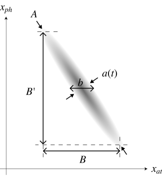
Figure 3: The density plot of the one-dimensional Gaussian model to the total squared two-particle atom-photon wave function in Eq. (24), with $x_{at}$ and $x_{ph}$ denoting the one-dimensional atom and photon coordinates. Here $A=c/\gamma$ gives the width of the relative proto-packet $|\Psi_{rel}|^{2}$ in Eq. (25) and $a(t)$ is the width of the CM proto-packet $|\Psi_{cm}|^{2}$ in Eq. (26). The coincidence width $\Delta x_{at}^{(c)}$ and the single width $\Delta x_{at}^{(s)}$ of the atom are given by $b$ and $B$ respectively, and $B^{\prime}$ is the single-particle width $\Delta x_{ph}^{(s)}$ of the photon.

As discussed above, $c/\gamma$ and $a(t)$ can be considered as the natural photonic and atomic wave packet widths found under the most often used assumptions: in the approximations of an infinitely heavy atom with the $\delta$-localized center-of-mass wave function for photonic wave packet, and in the case of a finite-mass non-excited and non-emitting atom for its spreading center-of-mass wave function. Any deviations from these natural widths can be considered as manifestations of entanglement in the two-particle system. To characterize these deviations, which are discussed below, it is convenient to introduce relative dimensionless widths

$$\delta r_{ph}^{(c)}(t)=\frac{\Delta r_{ph}^{(c)}(t)}{c/\gamma}\sim\frac{\eta(t)}{\sqrt{\eta^{2}(t)+v_{rec}^{2}/c^{2}}}$$ (36)

and

$$\delta r_{at}^{(c)}(t)=\frac{\Delta r_{at}^{(c)}(t)}{a(t)}\sim\frac{1}{\sqrt{1+\eta^{2}(t)}}.$$ (37)

The $``\text{natural}"$ values of these relative widths in a system without any entanglement are equal to one.

VI.2 Single-particle wave packet widths

In accordance with the definition of Eq. (30) the single-particle wave packets are related to the integrated squared absolute value of the two-particle wave function. There are two ways of performing the integrations over $\vec{r}_{at}$ or $\vec{r}_{ph}$ analytically. First, we can model the photon proto-packet in Eq. (25) by a Gaussian one. Then Eq. (24) takes the form of a product of two Gaussian packets with entangled variables and integration is carried out easily. We will use this method below in an analysis of the momentum-space wave packet. Here we will use another approach based on the consideration of two opposite cases, when one of two proto-packets in the product on the right-hand side of Eq. (24) is much narrower than the other one. Then the integrations can be carried out approximately, and the approximate expressions for the integrated absolute single-particle probability densities can be used for evaluation of the single-particle widths of wave packets.

In the case of a photon single-particle wave packet the squared absolute value of the two-particle wave function must be integrated over $\vec{r}_{at}$. Because of the forms of the entangled arguments of the atomic and photon proto-packets, in the case of integration over $\vec{r}_{at}$ the limits of relatively narrow and wide atomic proto-packets are separated by the conditions of small and large values of the control parameter $\eta(t)$ as defined in Eq. (34). With these conditions being used, the result of the integration takes the form

$$\frac{dw^{(s)}}{d\vec{r}_{ph}}=\int d\vec{r}_{at}\,\left|\vec{\Psi}(\vec{r}_{at},\vec{r}_{ph},t)\right|^{\,2}=\left\{\begin{array}[]{cl}\left|\Psi_{cm}(\vec{r}_{ph})\right|^{\,2}\,,&\quad\eta(t)\gg 1,\\[5.69054pt] \left|\Psi_{rel}\left(\vec{r}_{ph}\right)\right|^{\,2}\,,&\quad\eta(t)\ll 1,\end{array}\right.$$ (38)

where $\Psi_{rel}$ and $\Psi_{cm}$ are given by Eqs. (25) and (26), but the arguments of both functions in this case are identical and equal to $\vec{r}_{ph}$. The width of the single-particle photon wave packet (38) can be evaluated as

$$\Delta r_{ph}^{(s)}(t)\sim\max\left\{\frac{c}{\gamma},\;a(t)\right\}\sim\frac{c}{\gamma}\,\sqrt{1+\eta^{2}(t)}\,.$$ (39)

To describe the single-particle atomic wave packet, we must integrate Eq. (24) over ${\vec{r}}_{ph}$ (instead of ${\vec{r}}_{at}$). In this case, the regions of relatively narrow and wide atomic proto-packets are separated by the conditions that the control parameter $\eta(t)$ is either small or large compared to $v_{rec}/c$ rather than compared to one. This difference with the case of integration over $\vec{r}_{at}$ is related again to the form of the entangled argument of the atomic proto-packet in Eq. (24) discussed previously. The result of integration over $\vec{r}_{ph}$ is given by

$$\frac{dw^{(s)}}{d\vec{r}_{at}}=\int d\vec{r}_{ph}\,\left|\vec{\Psi}(\vec{r}_{at},\vec{r}_{ph},t)\right|^{\,2}\approx\left\{\begin{array}[]{ll}\left|\Psi_{cm}(\vec{r}_{at})\right|^{\,2}\,,&\quad\eta(t)\gg v_{rec}/c\\[5.69054pt] \left|\Psi_{rel}\left(-\frac{c}{v_{rec}}\,\vec{r}_{at}\right)\right|^{\,2}\,,&\quad\eta(t)\ll v_{rec}/c\ .\end{array}\right.$$ (40)

The width of this wave packet is evaluated as

$$\Delta r_{at}^{(s)}(t)\sim\max\left\{\frac{v_{rec}}{\gamma},\;a(t)\right\}\sim a(t)\,\frac{\sqrt{\eta^{2}(t)+v_{rec}^{2}/c^{2}}}{\eta(t)}.$$ (41)

In analogy with Eqs. (36) and (37) we can introduce the single-particle relative widths of the photon and atomic wave packets

$$\delta r_{ph}^{(s)}(t)=\frac{\Delta r_{ph}^{(s)}(t)}{c/\gamma}\sim\sqrt{1+\eta^{2}(t)}$$ (42)

and

$$\delta r_{at}^{(s)}(t)=\frac{\Delta r_{at}^{(s)}(t)}{a(t)}\sim\frac{\sqrt{\eta^{2}(t)+v_{rec}^{2}/c^{2}}}{\eta(t)}.$$ (43)

By comparing these results with those of Eqs. (36) and (37) we find the following group of fundamental reciprocity relations between the photon vs. atomic, and coincidence vs. single-particle, relative wave packet widths:

$$\delta r_{at}^{(c)}(t)\sim\frac{1}{\delta r_{ph}^{(s)}(t)}\quad\text{and}\quad\delta r_{ph}^{(c)}(t)\sim\frac{1}{\delta r_{at}^{(s)}(t)}.$$ (44)

Eqs. (44) show that it is possible to find the coincidence (conditional) wave packet widths without using the coincidence-scheme measurements. It is sufficient to measure both single-particle widths $\delta r_{ph}^{(s)}$ and $\delta r_{at}^{(s)}$, and then the coincidence widths can be found directly from Eqs. (44) without any further measurements. More explicitly, we can rewrite Eqs. (44) into $\Delta r_{at}^{(c)}\Delta r_{ph}^{(s)}\sim\Delta r_{ph}^{(c)}\Delta r_{at}^{(s)}\sim a(t)(c/\gamma)$. Note that $\eta(t)=a(t)/(c/\gamma)$ is essentially the aspect ratio of the wave packet’s $r_{ph}-r_{at}$ distribution. This definition is rather general: it is valid also for the momentum widths considered below in Section VIII, as well as for any other pairs of particles.

VI.3 Entanglement-induced anomalous narrowing and broadening of wave packets

The coincidence and single-particle relative widths of photon wave packets in the coordinate representation are plotted altogether in Fig. 4 in their dependence on the control parameter $\eta(t)$. The same curves describe atomic and photon wave packets in the momentum representation, as mentioned below near the end of Section VIII.

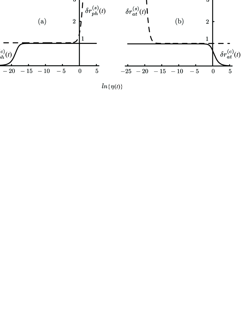
Figure 4: Coincidence (solid lines) and single-particle (dashed lines) relative widths of (a) photon and (b) atomic wave packets in the coordinate representation. We have used $v_{rec}/c=10^{-8}$.

The curves of Fig. 4 show that there are two regions of small and large values of the parameter $\eta(t)$ where either $\delta r^{(c)}\ll 1$ or $\delta r^{(s)}\gg 1$. These are the regions of entanglement-induced narrowing of the coincidence and broadening of the single-particle wave packets. As is seen from comparison of Figs. 4(a) and 4(b), for photon and atomic wave packets the regions of narrowing and broadening are oppositely located.

As an example, let us discuss the physics of these phenomena by using the photon wave packet widths as shown in Fig. 4(a). In this case the entanglement-induced narrowing for the coincidence photon wave packet occurs for $\eta<v_{rec}/c\ll 1$. Qualitatively this effect can be explained by combining the Doppler effect with the Heisenberg uncertainty relation JHE ; JHE1 . According to the latter, the size $a(t)$ of the atomic wave function corresponds to the velocity uncertainty of the atomic center of mass $\Delta v=1/Ma(t)$. Owing to the Doppler effect this gives rise to broadening of the spectrum of emitted photons up to the width $\delta\omega=k\Delta v=\omega_{0}/Mca(t)=v_{rec}/a(t)$. If $\eta(t)<v_{rec}/c$, this broadening exceeds the natural spectral width of the emitted light, i.e., $\delta\omega>\gamma$. As the photons of all frequencies are emitted coherently, integration over $\omega$ in the interval $\delta\omega$ shortens the effective emission time and spatial size of the emitted photon wave packet down to $t_{eff}=1/\delta\omega=a(t)/v_{rec}$ and $\Delta r_{ph}=ct_{eff}=(c/\gamma)(c\eta(t)/v_{rec})$. They are respectively much smaller than $\gamma^{-1}$ and $c/\gamma$ if $\eta(t)\ll v_{rec}/c$. It should be emphasized that the entanglement-induced wave-packet narrowing can be observed only in the coincidence scheme of measurements. Fig. 4(a) shows that under the same condition when $\delta r_{ph}^{(c)}<1$ (at $\eta(t)\ll v_{rec}/c$ or, more specifically, $ln\{\eta(t)\}\lesssim-18$) the relative width of the single-particle photon wave packet (the dashed line) remains equal to one, which corresponds to $\Delta r_{ph}^{(s)}=c/\gamma$.

The relation between the coincidence and single particle widths can also be illustrated by the depiction in Fig. 5(a).

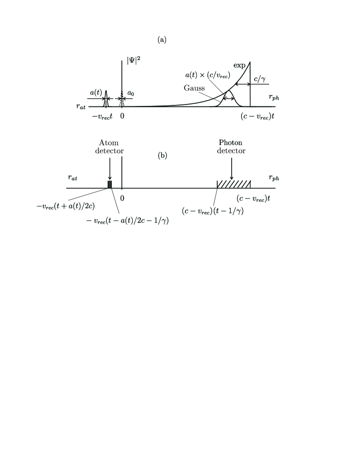
Figure 5: (a) Entanglement-induced narrowing of the photon wave packet to be measured in the coincidence scheme and (b) the regions where the atom and photon detectors have to be installed.

The exponential curve with a sharp edge corresponds to the photon proto-packet $|\Psi_{ph}^{(0)}(\vec{r}_{ph}-\vec{r}_{at})|^{2}$ given by Eq. (25) in its dependence on $\vec{r}_{ph}$. The dotted line is the initial atomic wave packet $|\Psi_{at}^{(0)}(\vec{r}_{at})|^{2}$. Two Gaussian solid-line curves describe the atomic proto-packet $|\Psi_{at}^{(0)}(\vec{R})|^{2}$ of Eq. (26) at $t\neq 0$ in its dependence on $\vec{r}_{at}$ at a given $\vec{r}_{ph}$ (the left curve) and on $\vec{r}_{ph}$ at a given $\vec{r}_{at}$ (the right curve). Relative locations of peaks of these two Gaussian curves are determined by the condition $\vec{R}=0$, where $\vec{R}$ is defined by Eq. (22) as the argument of the atomic proto-packet (26). The total two-particle wave function $\Psi(\vec{r}_{ph},\vec{r}_{at},t)$ of Eq. (24) differs from zero only if the $\vec{r}_{ph}$-dependent exponential and Gaussian curves overlap with each other. The conditions of their overlapping are illustrated in Fig. 5(b). In this picture the left shaded area indicates a zone for the atomic detector to be installed. In this case the $\vec{r}_{ph}$-dependent Gaussian function overlaps with the exponential one and under the condition $\eta<v_{rec}/c$ the first of these two curves is narrower than the second one. The total wave packet, equal to the product of the Gaussian and exponential functions, has the width of the narrower one, i.e., of the Gaussian function, and this width is smaller than than $c/\gamma$. However, if we change the atomic detector position, the position of the maximum of the Gaussian curve changes also. The summation of all contributions from various positions of the atomic detector corresponds to the transition from coincidence to single-particle measurements and returns us to the wide exponential curve with the width $c/\gamma$.

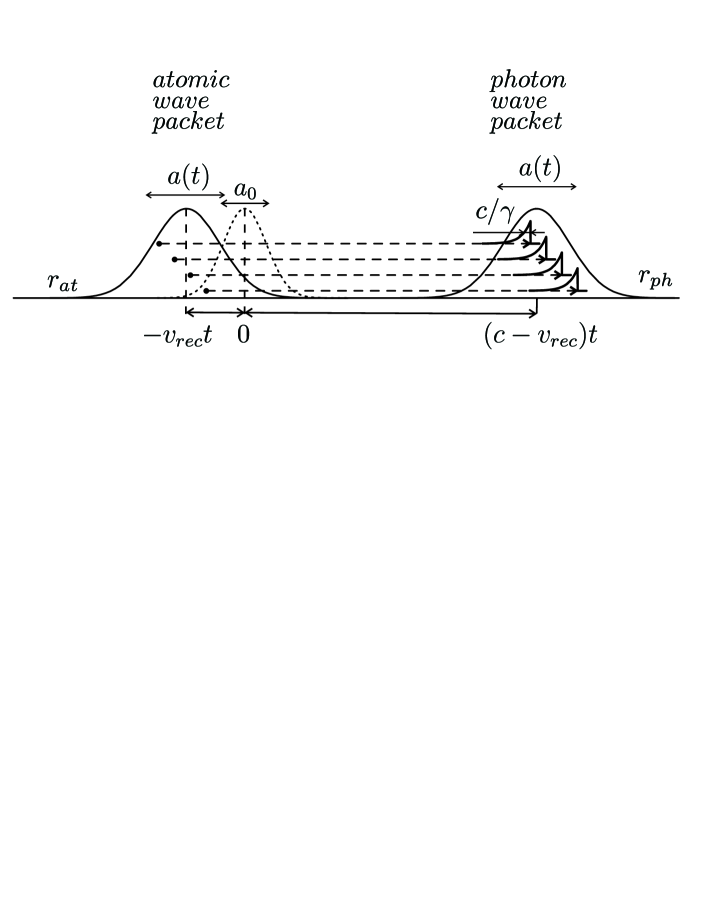
Figure 6: Entanglement-induced broadening of the photon wave packet.

The second new effect illustrated by Figs. 4 and 6 is the entanglement-induced broadening of the single-particle photon wave packet at large values of the control parameter, $\eta(t)>1$. Actually, the meaning of the st Fig. 6 is practically the same as that of Fig. 5(a). However, the main difference is that the atomic wave packet is taken very wide now. The dotted line describes the initial atomic wave packet. Big dots indicate possible positions of the atomic detector. At any given position of the atomic detector the photon wave packet to be measured has an exponential form and the width $c/\gamma$. However, when contributions from all positions of the atomic detector are summed together, this gives a wide Gaussian curve for the single-particle photon wave packet to be observed (the solid-line wide Gaussian curve at the right-hand side of the picture in Fig. 6). The width of this wide photon wave packet is $\Delta r_{ph}^{(s)}=a(t)$.

Note that the entanglement-induced broadening of the single-particle photon wave packet can occur even when the atomic mass $M$ is taken infinitely large, if only the atomic center-of-mass wave packet is wide enough, $a(t)>c/\gamma$ or $\eta(t)>1$.

VII Quantification of entanglement and the $R$-parameter

A convenient measure of the degree of pure-state two-particle entanglement, calculated in a number of previous studies JHE ; JHE1 ; PRA ; LANL ; Kazik , is the Schmidt number $K$ introduced in Grobe-etal94 ,

$$K=\frac{1}{\text{Tr}_{ph}\big{(}\hat{\rho}^{2}_{ph}\big{)}}=\frac{1}{\text{Tr}_{at}\big{(}\hat{\rho}^{2}_{at}\big{)}}\,,$$ (45)

where $\hat{\rho}_{ph}$ and $\hat{\rho}_{at}$ are the reduced density matrices

$$\hat{\rho}_{ph}=\text{Tr}_{at}\big{(}|\Psi\rangle\langle\Psi|\big{)},\quad\hat{\rho}_{at}=\text{Tr}_{ph}\big{(}|\Psi\rangle\langle\Psi|\big{)}\,,$$ (46)

Tr denotes trace with respect to either atomic or photon variables, and $|\Psi\rangle$ is given by Eq. (13). Note that $K$ essentially counts the number of effective Schmidt modes in the Schmidt decomposition of $\Psi$ Grobe-etal94 .

On the other hand, by analogy with our earlier discussion of ionization and dissociation PRA , we can also characterize the extent of the entanglement that can be seen in coincidence - single-particle measurements by the ratio $R(t)$ of the single-particle to coincidence widths of the particles’ wave packets. For spontaneous emission this parameter is given by

$$R(t)=\displaystyle\frac{\Delta r_{ph}^{(s)}}{\Delta r_{ph}^{(c)}}=\displaystyle\frac{\Delta r_{at}^{(s)}}{\Delta r_{at}^{(c)}}=\displaystyle\sqrt{\eta(t)+\frac{1}{\eta(t)}\left(\frac{v_{rec}}{c}\right)^{2}}\times\sqrt{\eta(t)+\frac{1}{\eta(t)}}.$$ (47)

The dependence of $R(t)$ on the control parameter $\eta(t)$ is shown in Fig. 7. The parameter $R$ is large at both small and large values of the control parameter $\eta(t)$, i.e., just where the above-described entanglement-induced narrowing or broadening of wave packets occur. At intermediate values of $\eta(t)$, $R\approx 1$.

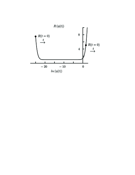
Figure 7: The parameter $R(t)$ vs. the control parameter $\eta(t)$.

Because the atomic center-of-mass wave packet spreads as time evolves, both $\eta(t)$ and $R(t)$ change with time. When the atomic wave packet spreads, $a(t)$ grows with time $t$ whereas the width of the photon proto-function remains constant and equals $c/\gamma$. For this reason, in the case of spontaneous emission the control parameter $\eta(t)$ is always a growing function of $t$. This contrasts with the case of photoionization PRA in which, depending on the initial conditions, $\eta(t)$ can be either an increasing or a decreasing function. This difference finds its reflection in the time evolution of the parameter $R(t)$. The direction of the time evolution of $R(t)$ is shown by arrows in Fig. 7 (always to the right!), whereas the dots indicate two possible initial values of this parameter, $R_{0}\equiv R(t=0)$, occurring immediately after the photon emission. In contrast to this, in the case of photoionization PRA , the time evolves either to the right (for $R_{0}$ located at the left wing of the curve of Fig. 7) or to the left (for $R_{0}$ located at the right wing). The second difference between spontaneous emission and photoionization concerns the limiting value of $R$ as $t\rightarrow\infty$. In the case of photoionization $\eta(\infty)$ is finite and $R(t\rightarrow\infty)=R_{0}$ PRA . In the case of spontaneous emission, as the function $\eta(t)$ monotonously grows, the parameter $R$ grows without limit: $R\left(\eta(t)\right)\rightarrow\infty$. These differences show that there is no complete identity between the cases of two massive particles and a massive plus a massless one.

The relation between the parameter $R$ and entanglement is dynamical and not direct. In the case of unentangled states $R\equiv 1$, which means that deviations of $R$ from unity are related to the entanglement. On the other hand, the parameter $R$ depends on time, whereas in entangled states of non-interacting particles the degree of entanglement remains constant. This can be seen clearly in calculations of the Schmidt number $K=const$ JHE ; JHE1 ; PRA ; LANL ; Kazik . On the other hand, by modelling the atomic proto-packet of Eq. (25) by the Gaussian expressions, in a way similar to that of Ref. LANL , we can show that $R_{0}=K$. This means that initially the parameter $R$ coincides with the Schmidt number and shows explicitly the degree of entanglement of the two-particle state formed immediately after the decay. Later the parameter $R$ evolves as described above owing to spreading of the atomic proto-function wave packet. If initially $R_{0}>1$ and if at some time the parameter $R(t)$ approaches one, the time region where $R(t)\approx 1$ can be referred to as the hidden-entanglement region LANL . In this case the Schmidt number $K$ and the entanglement itself remain as high as that at $t=0$, but the entanglement cannot be seen or measured via the comparison of single-particle and coincidence photon or atomic coordinate wave packet widths.

Here we recall the remarks at the end of Sec. III. We see that by substituting $v_{rec}/c$ with $m_{e}/m_{i}$, Eq. (47) gives the $R(t)$ of photoionization PRA . Now we also see that, by taking the limit $v_{rec}/c\rightarrow 1$, Eq. (47) is reduced to that describing the Schmidt number $K$ for the process of 1D down-conversion Law-Eberly04 (in the two-dimensional case the down-conversion $K$ equals the square of the one-dimensional $K$).

VIII Wave packets in the momentum representation

The widths of photon and atomic wave packets in the momentum representation is determined by the two-particle atom-photon momentum wave function determined by Eqs. (16) and (15).

$$\Psi^{(mom)}({\vec{q},\,\vec{k}\,}) = \left(\displaystyle\frac{L}{2\pi}\right)^{3}\,C^{(W-W)}_{\vec{q},\,\vec{k}}$$ (48)

$$\approx -i\displaystyle\frac{e\,z_{eg}\,\omega_{0}\,a_{0}^{3/2}\sin\vartheta_{k}}{2\pi\sqrt{\omega_{k}}\;\pi^{3/4}}\left(-\frac{\vec{q}\cdot\vec{k}}{M}+\omega_{k}-\omega_{0}+\frac{i\gamma}{2}\right)^{-1}\exp\left(-\displaystyle\frac{a_{0}^{2}({\vec{q}}+{\vec{k}})^{2}}{2}\right).\quad$$

For analytical calculations it’s convenient to substitute the Lorentzian factor by a Gaussian one

$$\Psi^{(mom)}({\vec{q},\,\vec{k}\,})\Rightarrow-i\displaystyle\frac{e\,z_{eg}\,\omega_{0}\,a_{0}^{3/2}\sin\vartheta_{k}}{\pi\sqrt{\omega_{k}}\pi^{3/4}\gamma}\,\exp\left\{-\frac{1}{2\gamma^{2}}\left(-\frac{\vec{q}\cdot\vec{k}}{M}+\omega_{k}-\omega_{0}\right)^{2}-\displaystyle\frac{a_{0}^{2}({\vec{q}}+{\vec{k}})^{2}}{2}\right\}.$$ (49)

By assuming that the vectors ${\vec{q}}$ and ${\vec{k}}$ are parallel to each other and to the observation direction, we can find easily from Eq. (49) both coincidence and single-particle atomic and photon wave packet widths in the momentum representation:

$$\Delta q^{(c)} \sim \min\left\{\frac{1}{a_{0}},\;\frac{\gamma Mc}{\omega_{0}}\right\}\sim\frac{\eta_{0}}{a_{0}}\left(\frac{v_{rec}^{2}}{c^{2}}+\eta_{0}^{2}\right)^{-1/2}\,,$$

$$\Delta q^{(s)} \sim \max\left\{\frac{1}{a_{0}},\;\frac{\gamma}{c}\right\}\sim\frac{1}{a_{0}}\sqrt{1+\eta_{0}^{2}}\,,$$ (50)

where $\eta_{0}$ is the value of the parameter $\eta(t)$ defined in Eq. (34) at $t=0$,

$$\eta_{0}\equiv\eta(t=0)=\displaystyle\frac{\gamma a_{0}}{c}\,,$$ (51)

and

$$\Delta k^{(c)} \sim \min\left\{\frac{1}{a_{0}},\;\frac{\gamma}{c}\right\}\sim\displaystyle\frac{\gamma/c}{\sqrt{1+\eta_{0}^{2}}}\,,$$

$$\Delta k^{(s)} \sim \max\left\{\frac{\gamma}{c},\;\frac{\omega_{0}}{Mc^{2}a_{0}}\right\}\sim\frac{\gamma/c}{\eta_{0}}\sqrt{\frac{v_{rec}^{2}}{c^{2}}+\eta_{0}^{2}}\,$$ (52)

In contrast to the coordinate wave packet widths the momentum wave packet widths are independent of time. By introducing the relative momentum wave packet widths (both coincidence and single-particle)

$$\delta q=\frac{\Delta q}{a_{0}^{-1}},\qquad\delta k=\frac{\Delta k}{\gamma/c}\,,$$ (53)

we find a second group of reciprocity relations

$$\delta k^{(c)}\sim\frac{1}{\delta q^{(s)}}\quad\text{and}\quad\delta q^{(c)}\sim\frac{1}{\delta k^{(s)}}.$$ (54)

By comparing directly the expressions (VIII) and (VIII) for the momentum wave packet widths with Eqs. (36), (37), (42), and (43) for the coordinate widths, we find the following series of identities:

$$\delta q^{(c)}\sim\delta r_{ph}^{(c)}(t=0), \delta q^{(s)}\sim\delta r_{ph}^{(s)}(t=0),$$

$$\delta k^{(c)}\sim\delta r_{at}^{(c)}(t=0), \delta k^{(s)}\sim\delta r_{at}^{(s)}(t=0).$$ and (55)

Because of these identity relations the dependencies of the momentum widths on $\eta_{0}$ coincide with the dependencies on $\eta(t)$ of the corresponding coordinate widths. With this understanding, the reader will be able to see that Fig. 4 remains just the same in the momentum representation, after appropriate replacement of the coordinate variances with momentum variances, and $\eta$ replaced with $\eta_{0}$ as horizontal axis label.

Again, as in the case of position-dependent wave packets, Eqs. (54) can be used for finding the coincidence (conditional) momentum-space wave packet widths $\Delta k^{(c)}$ and $\Delta q^{(c)}$ from the single-particle widths $\Delta k^{(s)}$ and $\Delta q^{(s)}$, without any coincidence-scheme measurements.

IX Entanglement and uncertainty relations

From the identities (VIII) and reciprocity relations (44) and (54), combined with the explicit definitions of the parameter $R(t)$ in Eq. (47) and the wave packet widths in Eqs. (32), (33), (39), (41), (VIII) and (VIII), we can find easily the following relation between the entanglement parameter $K=R(t=0)$ and the widths products

$$K=R(t=0) = \displaystyle\sqrt{\eta_{0}+\frac{1}{\eta_{0}}\left(\frac{v_{rec}}{c}\right)^{2}}\times\sqrt{\eta_{0}+\frac{1}{\eta_{0}}}$$ (56)

$$\sim \Delta r_{ph}^{(s)}(0)\times\Delta k^{(s)}\sim\Delta r_{at}^{(s)}(0)\times\Delta q^{(s)}$$

$$\sim \frac{1}{\Delta r_{ph}^{(c)}(0)\times\Delta k^{(c)}}\sim\frac{1}{\Delta r_{at}^{(c)}(0)\times\Delta q^{(c)}}\gtrsim 1\,.$$

The uncertainty relations following from these equations are

$$\Delta r_{ph}^{(s)}(0)\times\Delta k^{(s)}\sim K\gtrsim 1,\qquad\Delta r_{at}^{(s)}(0)\times\Delta q^{(s)}\sim K\gtrsim 1$$ (57)

and

$$\frac{1}{K}\sim\Delta r_{ph}^{(c)}(0)\times\Delta k^{(c)}\lesssim 1,\qquad\frac{1}{K}\sim\Delta r_{at}^{(c)}(0)\times\Delta q^{(c)}\lesssim 1.$$ (58)

Inequalities (57) represent the well-known Heisenberg uncertainty relations for single-particle measurements of any particle’s coordinate and momentum, while inequalities (58) establish quite different relations between the particle’s conditional coordinate and momentum uncertainties. These uncertainty relations restrict the products of such uncertainties from above: the uncertainty products are equal to (on the order of) the inverse degree of entanglement $1/K$, and they cannot be larger than one. With a growing degree of entanglement the products of the conditional uncertainties fall. On the other hand, Eqs. (57) show that the values of the usual single-particle uncertainty products are equal to the degree of entanglement $K$. These products grow with a growing $K$, and they turn to unity only in the non-entangled states where $K=1$.

Of course, these conclusions do not contradict the usual Heisenberg inequalities because the coincidence coordinate and momentum wave packet widths are assumed to be found under different conditions. With these conditions specified explicitly, the uncertainty relations (58) can be written as

$$\Delta r_{ph}^{(c)}(0)|_{{\vec{r}}_{at}=const}\times\Delta k^{(c)}|_{\,{\vec{q}}=const}\lesssim 1,\qquad\Delta r_{at}^{(c)}(0)|_{{\vec{r}}_{ph}=const}\times\Delta q^{(c)}|_{\,{\vec{k}}=const}\lesssim 1.$$ (59)

Nevertheless, inequalities (59) determine a kind of law of nature which, as far as we know, has never been explicitly formulated. Examples of very small values of the coincidence uncertainty coordinate and momentum products have been presented in Refs. Kazik ; LANL and experimental observations have begun to be reported Howell . What is new in the present derivation is a rather general form of the relationship between the value of the uncertainty products and the degree of entanglement.

In some sense the conditional uncertainty relations (58) are in concord with the well-known (often termed paradoxical) prediction by Einstein, Podolsky, and Rosen EPR . Indeed, as it was shown in EPR , in entangled decaying bipartite systems momentum or coordinates of one particle can be measured more precisely than permitted by the Heisenberg uncertainty relation if prior to this appropriate measurements are done exclusively with the other particle. But, of course, in such a formulation there is a rather well pronounced difference with our approach. The conditional uncertainty relations (58) are based on the idea of coincidence measurements, i.e., simultaneous and joint measurements to be made with both particles.

Eqs. (58) and (59) are derived at $t=0$, and they are valid as long as the atomic wave packet does not significantly spread. It is interesting to check how do the derived relations change at longer $t$ or, in other words, whether the wave packet spreading modifies or violates the uncertainty relations (58) and (59). The general answer is no, there is no violation of the time-dependent coincidence uncertainty relations arising from the wave packet spreading. To show this we have to use explicit expressions for the time-dependent widths of the coordinate wave packets $\Delta r_{ph}^{(c)}(t)$ and $\Delta r_{at}^{(c)}(t)$ given in Eqs. (32) and (33) together with Eqs. (VIII) and (VIII) for $\Delta k^{(c),(s)}$ and $\Delta k^{(c),(s)}$. The results have the form

$$\Delta r_{ph}^{(c)}(t)\times\Delta k^{(c)}\sim\frac{\eta(t)}{\sqrt{\eta^{2}(t)+v_{rec}^{2}/c^{2}}}\times\frac{1}{\sqrt{\eta_{0}^{2}+1}}=\frac{1}{R(t)}\sqrt{\frac{\eta^{2}(t)+1}{\eta_{0}^{2}+1}}$$ (60)

and

$$\Delta r_{at}^{(c)}(t)\times\Delta q^{(c)}\sim\frac{1}{\sqrt{1+\eta^{2}(t)}}\times\frac{\eta_{0}}{\sqrt{\eta_{0}^{2}+v_{rec}^{2}/c^{2}}}.$$ (61)

As $\eta(t)\geq\eta_{0}$, Eqs. (60) and (61) show clearly that, indeed, the conditional uncertainty relations (59) remain valid at any $t$,

$$\Delta r_{ph}^{(c)}(t)\times\Delta k^{(c)}\lesssim 1,\qquad\Delta r_{at}^{(c)}(t)\times\Delta q^{(c)}\lesssim 1.$$ (62)

But Eqs. (60) and (61) indicate also some difference between the coincidence uncertainty products for atoms and photons in their dependence on time $t$. If the photon uncertainty coincidence product (60) monotonously grows with a growing $t$, though remaining smaller than one, the atomic coincidence uncertainty product (61) monotonously falls approaching zero at very large values of $\eta(t)$. This asymmetry is related to the zero photon mass and non-zero mass of an atom, which results in spreading atomic and non-spreading photon proto-functions (given,correspondingly by Eqs. (26) and (25)).

What is destroyed by spreading is a direct connection between conditional uncertainty products and the Schmidt number $K$, at $t=0$ given by Eq. (58). As $K=const$ and the photon conditional uncertainty product (60) is a growing function of $t$, owing to spreading this product becomes larger than $1/K$. On the other hand, the last form of Eq. (60) shows that this product is also larger than $1/R(t)$. Hence, at $t\neq 0$ the photon conditional uncertainty product appears to be restricted from both above and below

$$\max\left\{\frac{1}{K},\,\frac{1}{R(t)}\right\}<\Delta r_{ph}^{(c)}(t)\times\Delta k^{(c)}<1.$$ (63)

As for the atomic conditional uncertainty product, as it falls with a growing $t$, owing to spreading it becomes even smaller than $1/K$, and this restricts this product from above even stronger than without spreading (see Eq. (62))

$$\Delta r_{at}^{(c)}(t)\times\Delta q^{(c)}\lesssim\frac{1}{K}\lesssim 1.$$ (64)

X Experiment

Concerning related experiments, note first the two recent works  Howell ; Kulik on investigation of entanglement in the process of spontaneous parametric downconversion. We did not consider down-conversion in this paper at all. On the other hand, many results presented above are general enough to be valid for any pairs of particles. Definitely, one of such results is the relation between the degree of entanglement and the value of the product of coordinate and momentum conditional uncertainties (58). In the experiment  Howell this product was found to be about 0.2 which is clearly less than one. This result agrees with Eqs. (58) derived above, though the relation between the conditional uncertainty product and the Schmidt number $K$ or the wave packet width ratio $R$ were not checked experimentally. We think that such an additional experimental investigation would be very interesting.

As for experiments specifically on entanglement in spontaneous emission of a photon, the most closely related work is that by Kurtsiefer, et al. Kurt . In this experiment the atomic momentum wave packet arising after spontaneous emission of a photon was measured in the coincidence and single-particle schemes of measurements. The coincidence width was shown to be smaller than the single-particle one. But this is not yet a direct confirmation of our predictions. As shown above, at small values of the control parameter $\eta$ the coincidence (conditional) width of the atomic momentum wave packet $\Delta q^{(c)}$ falls below its natural value $a_{0}^{-1}$ equal to the same width for a non-emitting ground-state atom (Fig. 2(a)). To see this one has to provide conditions under which $\eta<v_{rec}/c$. Probably this requirement was not fulfilled in the experiment Kurt and for this reason the observed coincidence wave packet width remained larger than $a_{0}^{-1}$. This quick analysis shows that, first, observation of entanglement effects in atomic spontaneous emission is possible and, second, to observe these effects the experiment has to be further refined.

XI Conclusion

To summarize, the relationship between atom-photon wave packet structures and entanglement in spontaneous emission has been analyzed. Finite atomic mass and finite initial size of the atomic center-of-mass wave function were taken into account. Two new effects reported were anomalous narrowing and anomalous broadening of the coordinate atomic and photon wave packets as observed in the coincidence and single-particle schemes of measurements. Atomic and photon wave packets were investigated both in the coordinate and momentum representations and a series of symmetry relations for their widths were established. These relations and the definition of the parameters characterizing the degree of entanglement were used to establish that (a) the product of single-particle coordinate and momentum uncertainties is equal (or is of the order of) the Schmidt number $K$ and (b) the product of coincidence (conditional) coordinate and momentum uncertainties is equal or is of the order of the inverse Schmidt number, $1/K$. The second of these two results shows that the coincidence coordinate and momentum uncertainty product is always less than one, and this is in the spirit of the conclusion reached by EPR in their famous discussion.

- (1) V. Weisskopf and E. Wigner, Z. Phys. 63, 54 (1930).
- (2) K. Rza̧żewski and W. Żakowicz, J. Phys. B 25, L319 (1992).
- (3) K.W. Chan, C.K. Law and J.H. Eberly, Phys. Rev. Lett. 88, 100402 (2002).
- (4) K.W. Chan, C.K. Law and J.H. Eberly, Phys. Rev. A 68, 022110 (2003).
- (5) K.W. Chan, C.K. Law, M.V. Fedorov, and J.H. Eberly, J. Mod. Opt. 51, 1779 (2004).
- (6) H. Huang and J.H. Eberly, J. Mod. Opt. 40, 915 (1993).
- (7) M.H. Rubin, Phys. Rev. A 54, 5349 (1996).
- (8) C.H. Monken, P.H. Souto Ribeiro, and S. Padua, Phys. Rev. A 57, 3123 (1998); S.P. Walborn, A.N. de Oliveira, and C.H. Monken, Phys. Rev. Lett. 90, 143601 (2003).
- (9) A.F. Abouraddy, B.E.A. Saleh, A.V. Sergienko, and M.C. Teich, Phys. Rev. Lett. 87, 123602 (2001).
- (10) E.J.S. Fonseca, C.H. Monken, S. Pádua, and G.A. Barbosa, Phys. Rev. A 59, 1608 (1999).
- (11) C.K. Law, I.A. Walmsley and J.H. Eberly, Phys. Rev. Lett. 84, 5304 (2000).
- (12) C.K. Law and J.H. Eberly, Phys. Rev. Lett. 92, 127903 (2004).
- (13) M. D’Angelo, Y-H. Kim, S.P. Kulik, and Y. Shih, Phys. Rev. Lett. 92, 233601 (2004).
- (14) M.V. Fedorov, M.A. Efremov, A.E. Kazakov, K.W. Chan, C. K. Law and J. H. Eberly, Phys. Rev. A 69, 052117 (2004).
- (15) K.W. Chan and J.H. Eberly, quant-ph/0404093.
- (16) T. Opatrny, B. Beb, and G. Kurizki, Phys. Rev. Lett. 90, 250404 (2003).
- (17) T. Opatrny, M. Kolar, G. Kurizki, and B. Deb, Int. J. Quant. Inf. 2, 305 (2004).
- (18) P. Krekora, Q. Su and R. Grobe, J. Mod. Opt. (in press, 2004).
- (19) R. Grobe, K. Rza̧żewski, and J.H. Eberly, J. Phys. B 27, L503-L508 (1994).
- (20) C.K. Law, Phys. Rev. A (in press). !
- (21) K. Mishima, M. Hayashi, and S.H. Lin, Phys. Lett. A (in press, 2004).
- (22) M.D. Reid, Phys. Rev. A 40, 913 (1989). See also, M.D. Reid and P.D. Drummond, Phys. Rev. A 40, 4493 (1989).
- (23) A. Einstein, B. Podolsky and N. Rosen, Phys. Rev. 47, 777 (1935).
- (24) A.I. Akhiezer and V.B. Berestetskii, Quantum Electrodynamics (Interscience Publishers, 1965).
- (25) V.B. Berestetskii, E.M. Lifshitz, L.P. Pitaevskii, Relativistic Quantum Theory 1 (Pergamon Press, 1971).
- (26) L. Mandel and E. Wolf, Optical Coherence and Quantum Optics (Cambridge, University Press, 1995).
- (27) M.O. Scully and M.S. Zubairy, Quantum Optics (Cambridge, University Press, 1997).
- (28) OPN Trends, The Nature of Light. What Is a Photon? 3, No. 1, October 2003.
- (29) J.C. Howell, R.S. Bennink, S.J. Bentley, and R.W. Boyd, Phys. Rev. Lett. 92, 210403 (2004).
- (30) C. Kurtsiefer et al., Phys. Rev. A 55, R2539 (1997).