Entanglement and the Einstein-Podolsky-Rosen paradox with coupled intracavity optical downconverters

Abstract

We show that two evanescently coupled $\chi^{(2)}$ parametric downconverters inside a Fabry-Perot cavity provide a tunable source of quadrature squeezed light, Einstein-Podolsky-Rosen correlations and quantum entanglement. Analysing the operation in the below threshold regime, we show how these properties can be controlled by adjusting the coupling strengths and the cavity detunings. As this can be implemented with integrated optics, it provides a possible route to rugged and stable EPR sources.

I Introduction

The Einstein, Podolsky and Rosen (EPR) paradox stems from a famous paper published in $1935$ EPR , which showed that local realism is not consistent with quantum mechanical completeness. A direct and feasible demonstration of the EPR paradox with continuous variables was first suggested using nondegenerate parametric amplification (also known as the OPA) eprquad . The optical quadrature phase amplitudes used in these proposals have the same mathematical properties as the position and momentum originally used by EPR. Even though the correlations between these are not perfect, they are still entangled sufficiently to allow for an inferred violation of the uncertainty principle, which is equivalent to the EPR paradox eprMDR ; rd . An experimental demonstration of this proposal by Ou et al. soon followed, showing a clear agreement with quantum theory Ou .

In this work, rather than using the nondegenerate optical parametric oscillator (OPO), we consider an alternative device using two degenerate type I downconverters inside the same optical cavity, and coupled by evanescent overlaps of the intracavity modes within the nonlinear medium. Generally, such a device may be considered as either a single nonlinear crystal pumped by two spatially separated lasers, or two waveguides with a $\chi^{(2)}$ component. We calculate phase-dependent correlations between the two low frequency outputs of the cavity in the below threshold regime, showing that this system exhibits a wide range of behaviour and is potentially an easily tunable source of single-mode squeezing, entangled states and states which exhibit the EPR paradox. The spatial separation of the output modes means that they do not have to be separated by optical devices before measurements can be made, along with the unavoidable losses which would result from this procedure. The entangled beams produced can be degenerate in both frequency and polarisation, unlike those of the nondegenerate OPO, and would exit the cavity at spatially separated locations. These correlations are tunable by controlling some of the operational degrees of freedom of the system, including the evanescent couplings between the two waveguides, the input power and the cavity detunings.

The term nonlinear coupler was given to a system of two coupled waveguides without an optical cavity by Per̆ina et al. coupler . Generically, the device consists of two parallel optical waveguides which are coupled by an evanescent overlap of the guided modes. The quantum statistical properties of this device when the nonlinearity is of the $\chi^{(3)}$ type have been theoretically investigated, predicting energy transfer between the waveguides Ibrahim and the generation of correlated squeezing korea . Coupled $\chi^{(2)}$ downconversion processes in the travelling wave configuration have also been examined theoretically, predicting that light produced in one of the media can be controlled by light entering the other mista , and that such a device can produce entanglement of the output beams herec . The coupler with $\chi^{(2)}$ nonlinearity held inside a pumped Fabry-Perot cavity, and operating in the second harmonic generation (SHG) configuration, was introduced by Bache et al. dimer , who named it the quantum optical dimer by analogy with various systems that display coupling between discrete sites. They analysed intensity correlations between the modes, predicting noise suppression in both the sum and the difference.

As the intracavity $\chi^{(2)}$ downconversion processes have long been appreciated as sources of quantum states of the electromagnetic field (See Martinelli et al. bigpaul for an overview), we will combine and extend these previous analyses to consider two coupled downconverters operating inside a Fabry-Perot cavity. The advantage of this proposal is the all-integrated nature of the device, which promises greatly increased robustness. Additional potential advantages are the reductions in threshold pump power and phase noise, relative to current practise. Another potential advantage as compared to the normal type II polarisation nondegenerate OPO lies in the difficulty of stabilising this device at frequency degeneracy Fabre1 ; Fabre2 . Our proposal should be well stabilised by the linear coupling, without having to add any additional features.

II The system and equations of motion

The physical device we wish to examine differs from that described in Ref. dimer in one important detail. We will analyse it in the downconversion regime, where the cavity pumping is at a frequency $2\omega_{L}\simeq\omega_{b}$. As this device has been described in detail in Ref. dimer , we will give a briefer description of the essential features here. The system of interest consists of two coupled nonlinear $\chi^{(2)}$ waveguides inside a driven optical cavity, which may utilise integrated Bragg reflection for compactness. Each waveguide supports two resonant modes at frequencies $\omega_{a},\,\omega_{b}$, where $2\omega_{a}\simeq\omega_{b}$. The higher frequency modes at $\omega_{b}$ are driven coherently with an external laser, while the nonlinear interaction within the waveguides produces pairs of downconverted photons with frequency $\omega_{a}$ . We assume that only the cavity modes at these two frequencies are important and that there is perfect phase matching inside the media. The two waveguides are evanescently coupled as in Ref. dimer . Besides the differences in the pumping frequency, we will be interested in the phase-dependent correlations necessary to demonstrate entanglement and the EPR paradox, rather than the intensity correlations of Ref. dimer .

The effective Hamiltonian for the system can be written as

$${\mathcal{H}}_{eff}={\mathcal{H}}_{int}+{\mathcal{H}}_{couple}+{\mathcal{H}}_{pump}+{\mathcal{H}}_{res},$$ (1)

where the nonlinear interaction with the $\chi^{(2)}$ media is described by

$${\mathcal{H}}_{int}=i\hbar\frac{\kappa}{2}\left[\hat{a}_{1}^{{\dagger}\;2}\hat{b}_{1}-\hat{a}_{1}^{2}\hat{b}_{1}^{{\dagger}}+\hat{a}_{2}^{{\dagger}\;2}\hat{b}_{2}-\hat{a}_{2}^{2}\hat{b}_{2}^{{\dagger}}\right]\,\,.$$ (2)

Here $\kappa$ denotes the effective nonlinearity of the waveguides (we assume that the two are equal), and $\hat{a}_{k},\;\hat{b}_{k}$ are the bosonic annihilation operators for quanta at the frequencies $\omega_{a},\;\omega_{b}$ within the crystal $k\;(=1,2)$. The coupling by evanescent waves is described by

$${\mathcal{H}}_{couple}=\hbar J_{a}\left[\hat{a}_{1}\hat{a}_{2}^{{\dagger}}+\hat{a}_{1}^{{\dagger}}\hat{a}_{2}\right]+\hbar J_{b}\left[\hat{b}_{1}\hat{b}_{2}^{{\dagger}}+\hat{b}_{1}^{{\dagger}}\hat{b}_{2}\right],$$ (3)

where the $J_{k}$ are the coupling parameters at the two frequencies, as described in Ref. dimer . We note that in that work it is stated that the lower frequency coupling, $J_{a}$, is generally stronger than the higher frequency coupling, $J_{b}$, and also that values of $J_{a}$ as high as $50$ times the lower frequency cavity loss rate were calculated to be physically reasonable. The cavity pumping is described by

$${\mathcal{H}}_{pump}=i\hbar\left[\epsilon_{1}\hat{b}_{1}^{{\dagger}}-\epsilon_{1}^{\ast}\hat{b}_{1}+\epsilon_{2}\hat{b}_{2}^{{\dagger}}-\epsilon_{2}^{\ast}\hat{b}_{2}\right],$$ (4)

where the $\epsilon_{k}$ represent pump fields which we will describe classically. Finally, the cavity damping is described by

$${\mathcal{H}}_{res}=\hbar\sum_{k=1}^{2}\left(\Gamma_{a}^{k}\hat{a}_{k}^{{\dagger}}+\Gamma_{b}^{k}\hat{b}_{k}^{{\dagger}}\right)+h.c.,$$ (5)

where the $\Gamma^{k}$ represent bath operators at the two frequencies and we have made the usual zero temperature approximation for the reservoirs.

With the standard methods GardinerQN , and using the operator/c-number correspondences $(\hat{a}_{j}\leftrightarrow\alpha_{j},\hat{b}_{j}\leftrightarrow\beta_{j})$, the Hamiltonian can be mapped onto a Fokker-Planck equation for the Glauber-Sudarshan P-distribution Roy ; Sud . However, as the diffusion matrix of this Fokker-Planck equation is not positive-definite, it cannot be mapped onto a set of stochastic differential equations. Hence we will use the positive-P representation plusP which, by doubling the dimensionality of the phase-space, allows a Fokker-Planck equation with a positive-definite diffusion matrix to be found and thus a mapping onto stochastic differential equations. Making the correspondence between the set of operators $(\hat{a}_{j},\hat{a}_{j}^{{\dagger}},\hat{b}_{j},\hat{b}_{j}^{{\dagger}})$ $(j=1,2)$ and the set of c-number variables $(\alpha_{j},\alpha_{j}^{+},\beta_{j},\beta_{j}^{+})$, we find the following set of equations,

$$\frac{d\alpha_{1}}{dt} = -(\gamma_{a}+i\Delta_{a})\alpha_{1}+\kappa\alpha_{1}^{+}\beta_{1}+iJ_{a}\alpha_{2}+\sqrt{\kappa\beta_{1}}\;\eta_{1}(t),$$

$$\frac{d\alpha_{1}^{+}}{dt} = -(\gamma_{a}-i\Delta_{a})\alpha_{1}^{+}+\kappa\alpha_{1}\beta_{1}^{+}-iJ_{a}\alpha_{2}^{+}+\sqrt{\kappa\beta_{1}^{+}}\;\eta_{2}(t),$$

$$\frac{d\alpha_{2}}{dt} = -(\gamma_{a}+i\Delta_{a})\alpha_{2}+\kappa\alpha_{2}^{+}\beta_{2}+iJ_{a}\alpha_{1}+\sqrt{\kappa\beta_{2}}\;\eta_{3}(t),$$

$$\frac{d\alpha_{2}^{+}}{dt} = -(\gamma_{a}-i\Delta_{a})\alpha_{2}^{+}+\kappa\alpha_{2}\beta_{2}^{+}-iJ_{a}\alpha_{1}^{+}+\sqrt{\kappa\beta_{2}^{+}}\;\eta_{4}(t),$$

$$\frac{d\beta_{1}}{dt} = \epsilon_{1}-(\gamma_{b}+i\Delta_{b})\beta_{1}-\frac{\kappa}{2}\alpha_{1}^{2}+iJ_{b}\beta_{2},$$

$$\frac{d\beta_{1}^{+}}{dt} = \epsilon_{1}^{\ast}-(\gamma_{b}-i\Delta_{b})\beta_{1}^{+}-\frac{\kappa}{2}\alpha_{1}^{+\;2}-iJ_{b}\beta_{2}^{+},$$

$$\frac{d\beta_{2}}{dt} = \epsilon_{2}-(\gamma_{b}+i\Delta_{b})\beta_{2}-\frac{\kappa}{2}\alpha_{2}^{2}+iJ_{b}\beta_{1},$$

$$\frac{d\beta_{2}^{+}}{dt} = \epsilon_{2}^{\ast}-(\gamma_{b}-i\Delta_{b})\beta_{2}^{+}-\frac{\kappa}{2}\alpha_{2}^{+\;2}-iJ_{b}\beta_{1}^{+},$$ (6)

where the $\gamma_{k}$ represent cavity damping. We have also added cavity detunings $\Delta_{a,b}$ from the two resonances, so that for a pump laser at angular frequency $2\omega_{L}$, one has $\Delta_{a}=\omega_{a}-\omega_{L}$and $\Delta_{b}=\omega_{b}-2\omega_{L}$. Below, in section V, we will investigate detuning effects in greater detail. The real Gaussian noise terms have the correlations $\overline{\eta_{j}(t)}=0$ and $\overline{\eta_{j}(t)\eta_{k}(t^{\prime})}=\delta_{jk}\delta(t-t^{\prime})$. Note that, due to the independence of the noise sources, $\alpha_{k}\;(\beta_{k})$ and $\alpha_{k}^{+}\;(\beta_{k}^{+})$ are not complex conjugate pairs, except in the mean over a large number of stochastic integrations of the above equations. However, these equations do allow us to calculate the expectation values of any desired time-normally ordered operator moments, exactly as required to calculate spectral correlations.

III Linearised analysis

In an operating regions where it is valid, a linearised fluctuation analysis provides a simple way of calculating both intracavity and output spectra of the system DFW ; mjc , by treating it as an Ornstein-Uhlenbeck process ornstein . To perform this analysis we first divide the variables of Eq. 6 into a steady-state mean value and a fluctuation part, e.g. $\alpha_{1}\rightarrow\alpha_{1}^{ss}+\delta\alpha_{1}$ and so on for the other variables. We find the steady state solutions by solving the equations (6) without the noise terms (note that in this section we will treat all fields as being at resonance), and write the equations for the fluctuation vector $\delta\tilde{x}=[\delta\alpha_{1},\delta\alpha_{1}^{+},\delta\alpha_{2},\delta\alpha_{2}^{+},\delta\beta_{1},\delta\beta_{1}^{+},\delta\beta_{2},\delta\beta_{2}^{+}]^{T}$, to first order in these fluctuations, as

$$d\;\delta\tilde{x}=-A\delta\tilde{x}\;dt+BdW,$$ (7)

where the drift matrix is

$$A=\left[\begin{array}[]{cc}A_{aa}&-A_{ba}^{*}\\ A_{ba}&A_{bb}\end{array}\right],$$ (8)

with

$$A_{aa} = \left[\begin{array}[]{cccc}\gamma_{a}&-\kappa\beta_{1}^{ss}&-iJ_{a}&0\\ -\kappa\beta_{1}^{ss\ast}&\gamma_{a}&0&iJ_{a}\\ -iJ_{a}&0&\gamma_{a}&-\kappa\beta_{2}^{ss}\\ 0&iJ_{a}&-\kappa\beta_{2}^{ss\ast}&\gamma_{a}\end{array}\right],$$ (13)

$$A_{ba} = \left[\begin{array}[]{cccc}\kappa\alpha_{1}^{ss}&0&0&0\\ 0&\kappa\alpha_{1}^{ss\ast}&0&0\\ 0&0&\kappa\alpha_{2}^{ss}&0\\ 0&0&0&\kappa\alpha_{2}^{ss\ast}\end{array}\right],$$ (18)

$$A_{bb} = \left[\begin{array}[]{cccc}\gamma_{b}&0&-iJ_{b}&0\\ 0&\gamma_{b}&0&iJ_{b}\\ -iJ_{b}&0&\gamma_{b}&0\\ 0&iJ_{b}&0&\gamma_{b}\end{array}\right].$$ (23)

In this equation, $dW$ is a vector of real Wiener increments, and the matrix $B$ is zero except for the first four diagonal elements, which are respectively $\sqrt{\kappa\beta_{1}^{ss}},\;\sqrt{\kappa\beta_{1}^{ss\ast}},\;\sqrt{\kappa\beta_{2}^{ss}},\;\sqrt{\kappa\beta_{2}^{ss\ast}}$. The essential conditions for this expansion to be valid are that moments of the fluctuations be smaller than the equivalent moments of the mean values, and that the fluctuations stay small. In the case of the single optical parametric oscillator (OPO), it is well known that there is a critical operating point around which this condition does not hold. This point is easily found by examination of the eigenvalues of the equivalent fluctuation drift matrix for that system, and this procedure is also valid in the present case. The fluctuations will not tend to grow as long as none of the eigenvalues of the matrix $A$ develop a negative real part. At the point at which this happens the linearised fluctuation analysis is no longer valid, as the fluctuations can then grow exponentially and the necessary conditions for linearisation are no longer fulfilled. In this work we will only be interested in a region where linearisation is valid.

To examine the stability of the system, we first need to find the steady state solutions for the amplitudes, by solving for the steady state of Eq. 6 with the noise terms dropped. As in the usual optical parametric oscillator, there is an oscillation threshold below which $\alpha_{j}^{ss}=0$ and only the high frequency mode is populated. In the present case, for a real pump, we find $\beta_{j}^{ss}=\epsilon/(\gamma_{b}-iJ_{b})$. Inserting these solutions in the matrix $A$ allows us to find simple expressions for the eigenvalues,

$$\lambda_{1,2} = \gamma_{b}+iJ_{b},$$

$$\lambda_{3,4} = \gamma_{b}-iJ_{b},$$

$$\lambda_{5,6} = \gamma_{a}+\sqrt{\left[\kappa^{2}\epsilon^{2}/\widetilde{\gamma}_{b}^{2}-J_{a}^{2}\right]},$$

$$\lambda_{7,8} = \gamma_{a}-\sqrt{\left[\kappa^{2}\epsilon^{2}/\widetilde{\gamma}_{b}^{2}-J_{a}^{2}\right]}.$$ (24)

Here we have introduced auxiliary variables, $\widetilde{\gamma}{}_{a,b}=\sqrt{\gamma_{a,b}^{2}+J_{a,b}^{2}}$. We immediately see that $\lambda_{7,8}$ can develop negative real parts for a pump amplitude greater than the critical value, $\epsilon_{c}=\widetilde{\gamma}{}_{a}\widetilde{\gamma}{}_{b}/\kappa$. As it must, this expression reduces to the single OPO expression of $\gamma_{a}\gamma_{b}/\kappa$ when the couplings are set to zero. In that case, there is then a stable above threshold solution in which the high frequency mode inside the cavity remains constant, independently of any further increase in the pumping, and the low frequency mode becomes occupied.

In the present case, it is not simple to find general expressions for these above threshold solutions analytically, but as we will concentrate our attention on the rich variety of below threshold behaviour which is exhibited, this is not important here. We note here that, unlike the single OPO case with a resonant cavity, the threshold pumping is not a constant for fixed cavity loss rates, but is a function of the coupling strengths between the two waveguides. Using the below threshold solutions, we may calculate any desired time normally-ordered spectral correlations inside the cavity using the simple formula

$$S(\omega)=\left(A+i\omega\openone\right)^{-1}BB^{\text{T}}\left(A^{\text{T}}-i\omega\openone\right)^{-1},$$ (25)

after which we use the standard input-output relations mjc to relate these to quantities which may be measured outside the cavity.

IV Quantum correlations

IV.1 Single mode squeezing

The first quantities we wish to calculate are the single mode quadrature squeezing spectra, to compare these with the well-known results for the normal uncoupled OPO. Defining the quadrature amplitudes as

$$\hat{X}_{j}^{\theta}=\hat{a}_{j}\mbox{e}^{-i\theta}+\hat{a}_{j}^{{\dagger}}\mbox{e}^{i\theta},$$ (26)

(where $j=1,2$), we will use the notation

$$\hat{X}_{j}^{0} = \hat{X}_{j},$$

$$\hat{X}_{j}^{\frac{\pi}{2}} = \hat{Y}_{j}.$$ (27)

We note here that the quadrature definitions do not need to specify whether it is mode $a$ or $b$ which is involved, as we do not find any interesting behaviour in the high frequency modes below threshold and hence will only present results for the low frequency modes. With this normalisation the coherent state value for the quadrature variances is one. To simplify our results we will assume that the pumping terms for each crystal are real and equal $(\epsilon_{1}=\epsilon_{2}=\epsilon)$.

The expressions for the below threshold low frequency quadrature variances in the single OPO case are well known osenhor , being

$$S_{X}^{\text{out}}(\omega) = 1+\frac{4\gamma_{a}\gamma_{b}\kappa\epsilon}{(\gamma_{a}\gamma_{b}-\kappa\epsilon)^{2}+\gamma_{b}^{2}\omega^{2}},$$

$$S_{Y}^{\text{out}}(\omega) = 1-\frac{4\gamma_{a}\gamma_{b}\kappa\epsilon}{(\gamma_{a}\gamma_{b}+\kappa\epsilon)^{2}+\gamma_{b}^{2}\omega^{2}},$$ (28)

and predicting zero-frequency squeezing which becomes perfect in the $Y$ quadrature as the pump approaches the critical threshold value, $\epsilon=\gamma_{a}\gamma_{b}/\kappa$, although the linearised analysis breaks down near this point. Note that the variances inside and outside the cavity are related by $S_{X}^{\text{out}}=1+2\gamma_{a}V(\hat{X})$. Our coupled system would be expected to exhibit the above values in the limit as $J_{a,b}\rightarrow 0$, which provides a standard for comparison with the analytical results. In the general case, we find that $S_{X_{1}^{\theta}}^{\text{out}}=S_{X_{2}^{\theta}}^{\text{out}}$, as expected. We also find that the coupling means that the intracavity high frequency field is no longer real, but has a phase given by $\Theta_{b}=\tan^{-1}(J_{b}/\gamma_{b})$.

This will mean that the optimum correlations will no longer generally be found in the $X_{j}$ and $Y_{j}$ quadratures, but at some other phase angle, as found previously for second harmonic generation in detuned cavities granja . Experimentally, this does not present a problem as the local oscillator phase is normally swept across all angles, which must therefore include the optimum angle. We can find analytical solutions for the angle of maximum single-mode squeezing (and antisqueezing), for example, these differing by $\pi/2$ and being found as

$$\theta_{opt}=\tan^{-1}\left\{\frac{2V(\hat{X},\hat{Y})}{V(\hat{Y})-V(\hat{X})\pm\sqrt{\left[V(\hat{Y})-V(\hat{X})\right]^{2}+4\left[V(\hat{X},\hat{Y})\right]^{2}}}\right\},$$ (29)

where $V(A,B)=\langle AB\rangle-\langle A\rangle\langle B\rangle$. However, as this expression is a complicated function of several variables when written out in full, and will not necessarily give the optimum choices at all frequencies, nor when we consider correlations between the modes, we will present results where the local oscillator angle has been optimised numerically.

The $\hat{X}$ and $\hat{Y}$ spectral variances outside the cavity are found as

$$S_{X_{1,2}}^{\text{out}}(\omega) = 1+\frac{4\gamma_{a}\kappa\epsilon\left\{\gamma_{b}\left[\widetilde{\gamma_{b}}^{2}(\omega^{2}-J_{a}^{2})+J_{b}^{2}\gamma_{a}^{2}+(\gamma_{a}\gamma_{b}+\kappa\epsilon)^{2}\right]+2\gamma_{a}J_{b}^{2}\kappa\epsilon\right\}}{4\gamma_{a}^{2}\widetilde{\gamma_{b}}^{4}\omega^{2}+\left[\widetilde{\gamma_{b}}^{2}(\widetilde{\gamma_{a}}^{2}-\omega^{2})-\kappa^{2}\epsilon^{2}\right]^{2}},$$

$$S_{Y_{1,2}}^{\text{out}}(\omega) = 1-\frac{4\gamma_{a}\kappa\epsilon\left\{\gamma_{b}\left[\widetilde{\gamma_{b}}^{2}(\omega^{2}-J_{a}^{2})+J_{b}^{2}\gamma_{a}^{2}+(\gamma_{a}\gamma_{b}-\kappa\epsilon)^{2}\right]+2\gamma_{a}J_{b}^{2}\kappa\epsilon\right\}}{4\gamma_{a}^{2}\widetilde{\gamma_{b}}^{4}\omega^{2}+\left[\widetilde{\gamma_{b}}^{2}(\widetilde{\gamma_{a}}^{2}-\omega^{2})-\kappa^{2}\epsilon^{2}\right]^{2}},$$ (30)

which, as expected, reduce to the single OPO expressions above (28) when the coupling terms are set to zero. The output covariance is

$$V(\hat{X}_{j},\hat{Y}_{j})=\frac{4\gamma_{a}J_{b}\kappa\epsilon\left[\widetilde{\gamma}_{b}^{2}(\gamma_{a}^{2}-J_{a}^{2}+\omega^{2})+\kappa^{2}\epsilon^{2}\right]}{4\gamma_{a}^{2}\widetilde{\gamma_{b}}^{4}\omega^{2}+\left[\widetilde{\gamma_{b}}^{2}(\widetilde{\gamma_{a}}^{2}-\omega^{2})-\kappa^{2}\epsilon^{2}\right]^{2}},$$ (31)

which will give $\theta_{opt}=0,\pi/2$ for the uncoupled case, where $\hat{Y}$ is the squeezed quadrature and $\hat{X}$ the antisqueezed quadrature.

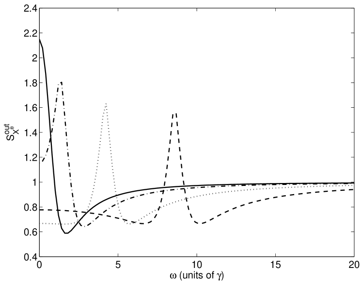
Figure 1: $S_{X^{\theta}}^{\text{out}}(\omega)$ for $\gamma=1$, $J_{b}=1$ and different $J_{a}$, all at the $\theta$ of maximum squeezing. The solid line is for $J_{a}=1$ and $\theta=113^{o}$, the dash-dotted line is $J_{a}=2$, the dotted line is $J_{a}=5$ and the dashed line is $J_{a}=10$, all for $\theta=22^{o}$. The pump amplitude is $\epsilon=0.5\epsilon_{c}$ in each case and all quantities plotted in this and subsequent graphics are dimensionless. Note that all plotted spectra are symmetric about zero frequency and all results shown use the value $\kappa=0.01$ and $\gamma_{a}=\gamma_{b}=\gamma$.

In Fig. 1 we show the single-mode output spectral quadrature variances for the quadrature of best squeezing as the low-frequency mode coupling strength is varied, beginning with $J_{a}=J_{b}=\gamma_{a}=\gamma_{b}=\gamma$. We note here that the pump values used in all the displayed results, $\epsilon_{j}=0.5\epsilon_{c}$, depend on the couplings as stated above and are therefore different for different combinations of the couplings, but are all the same fraction of the threshold value. We find less single-mode squeezing than in the uncoupled case for the same ratio $\epsilon/\epsilon_{c}$, and also find that changing $J_{b}$ mainly serves to change the angle of maximum squeezing. Changing $J_{a}$ changes the frequency at which the maximum of squeezing is found. We see that this device is not as efficient at producing squeezed single-mode outputs as the normal OPO, but as we are interested in the quantum correlations between the two output modes, we will now examine these.

IV.2 Entanglement and the EPR paradox

An entanglement criterion for optical quadratures has been outlined by Dechoum et al. ndturco , following from criteria developed by Duan et al. Duan which are based on the inseparability of the system density matrix. A theoretical method to demonstrate the EPR paradox using quadrature amplitudes was developed by Reid eprMDR , using the mathematical similarities of the quadrature operators to the original position and momentum operators. We will briefly outline these criteria here and then apply them to our system, using the quadrature operators $\hat{X}_{j}$ and $\hat{Y}_{j}$. Note that even though these quadratures have the same mathematical properties as the canonical position and momentum operators for the harmonic oscillator, they correspond physically to the real and imaginary parts of the electromagnetic field, not its position and momentum.

To demonstrate entanglement between the modes, we define the combined quadratures $\hat{X}_{\pm}=\hat{X}_{1}\pm\hat{X}_{2}$ and $\hat{Y}_{\pm}=\hat{Y}_{1}\pm\hat{Y}_{2}$ and calculate the variances in these, which we may do analytically. Optimising the result for arbitrary phase angles is better performed numerically. Following the treatment of Ref. ndturco , entanglement is guaranteed provided that

$$S_{X_{\pm}}^{\text{out}}+S_{Y_{\mp}}^{\text{out}}<4.$$ (32)

We note here that the combined variance defined in this way has an obvious relationship with the well-known two-mode squeezed states which are produced, for example, by the nondegenerate OPO democrat1 ; democrat2 , but that the quadratures between which we find entanglement here are not the same as those which are entangled in that case, where these are $\hat{X}_{-}$ and $\hat{Y}_{+}$. In the present case, considering only the phase angles $\theta=0$ and $\pi/2$, we find entanglement with $\hat{X}_{+}$ and $\hat{Y}_{-}$. The two individual variances can be written as

$$S_{X_{\pm}}^{\text{out}} = S_{X_{1}}^{\text{out}}+S_{X_{2}}^{\text{out}}\pm 2V(\hat{X}_{1},\hat{X}_{2}),$$

$$S_{X_{\pm}}^{\text{out}} = S_{X_{1}}^{\text{out}}+S_{X_{2}}^{\text{out}}\pm 2V(\hat{Y}_{1},\hat{Y}_{2}).$$ (33)

The individual quadrature variances are given above (30), while for the covariances we find:

$$V(\hat{X}_{1},\hat{X}_{2})=\frac{-8J_{a}J_{b}\gamma_{a}^{2}\widetilde{\gamma}_{b}^{2}\kappa\epsilon}{{4\gamma_{a}^{2}\widetilde{\gamma}_{b}^{4}\omega^{2}+\left[\widetilde{\gamma}_{b}^{2}(\widetilde{\gamma_{a}}^{2}-\omega^{2})-\kappa^{2}\epsilon^{2}\right]^{2}}},$$ (34)

and $V(\hat{Y}_{1},\hat{Y}_{2})=-V(\hat{X}_{1},\hat{X}_{2})$, showing that the $\hat{X}$ quadratures are anticorrelated and the $\hat{Y}$ quadratures are correlated. Although these results allow us to write analytical expressions for the combined variances, these are rather bulky and not very enlightening, so we will not reproduce them here.

To optimise the degree of entanglement as a function of the quadrature phase angle, we investigate the output spectral correlation

$$S_{\theta}^{\text{out}}(\hat{X}_{-})+S_{\theta}^{\text{out}}(\hat{Y}_{+}),$$ (35)

where the $\hat{X}$ quadratures are at the angle $\theta$ and the $\hat{Y}$ quadratures at the angle $\theta+\pi/2$. What we find, as shown in Fig. 2, is that the degree of entanglement and the frequency at which it exists depend on the coupling strength $J_{a}$ while the optimum angle depends on $J_{b}$. When we hold $J_{a}$ constant and increase $J_{b}$, we find that the maximum of entanglement is always found at zero frequency, but that the optimum quadrature angle changes.

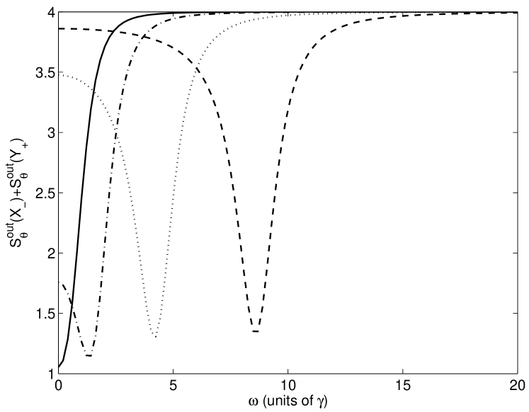
Figure 2: Demonstration of entanglement, using $S_{\theta}^{\text{out}}(\hat{X}_{-})+S_{\theta}^{\text{out}}(\hat{Y}_{+})$, for $\gamma=1$, $J_{b}=1$, and $J_{a}=1$ (solid line), $2$ (dash-dotted line), $5$ (dotted line) and $10$ (dashed line). The quadrature angle for $\hat{X}$ is $67^{o}$ and that for $\hat{Y}$ is $157^{o}$. The pump amplitude is $\epsilon=0.5\epsilon_{c}$.

To examine the utility of the system for the production of states which exhibit the EPR paradox, we follow the approach of Reid eprMDR . We assume that a measurement of the $\hat{X}_{1}$ quadrature, for example, will allow us to infer, with some error, the value of the $\hat{X}_{2}$ quadrature, and similarly for the $\hat{Y}_{j}$ quadratures. This allows us to make linear estimates of the quadrature variances, which are then minimised to give the inferred output variances,

$$S_{\text{inf}}^{\text{out}}(\hat{X}_{1}) = S_{X_{1}}^{\text{out}}-\frac{\left[V(\hat{X}_{1},\hat{X}_{2})\right]^{2}}{S_{X_{2}}^{\text{out}}},$$

$$S_{\text{inf}}^{\text{out}}(\hat{Y}_{1}) = S_{Y_{1}}^{\text{out}}-\frac{\left[V(\hat{Y}_{1},\hat{Y}_{2})\right]^{2}}{S_{Y_{2}}^{\text{out}}}.$$ (36)

The inferred variances for the $j=2$ quadratures are simply found by swapping the indices $1$ and $2$. As the $\hat{X}_{j}$ and $\hat{Y}_{j}$ operators do not commute, the products of the variances obey a Heisenberg uncertainty relation, with $S_{X_{j}}^{\text{out}}S_{Y_{j}}^{\text{out}}\geq 1$. Hence we find a demonstration of the EPR paradox whenever

$$S_{\text{inf}}^{\text{out}}(\hat{X}_{j})S_{\text{inf}}^{\text{out}}(\hat{Y}_{j})\leq 1.$$ (37)

With the expressions for the variances given in Eq. 30 and the covariances of Eq. 34, we have all we need to calculate the EPR correlations. Once again, however, the full expressions are somewhat unwieldy, so we will present the results graphically.

In Fig. 3 we present the results for optimised quadrature phase angles while $J_{b}$ is held constant at a value of $\gamma$ while $J_{a}$ is increased. Note that again the angle $\theta$ refers to the $\hat{X}^{\theta}$ quadratures, while the conjugate quadratures are at an angle of $\theta+\pi/2$. Changing $J_{b}$ serves to change the angle of the maximum violation, without changing the degree of violation, while changing $J_{a}$ changes both the degree and the frequency of the maximum violation. As expected, these results are the same for both outputs of the device.

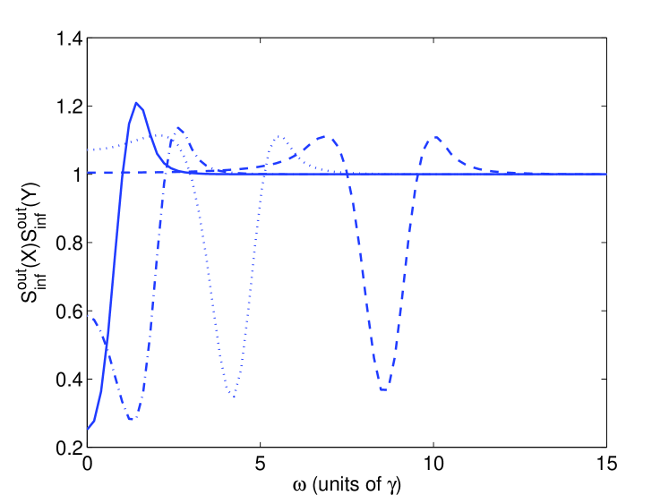
Figure 3: Demonstration of the EPR correlation for $J_{b}=\gamma=1$ and $J_{a}=1$ (solid line, $\theta=67^{o}$), $2$ (dash-dotted line, $\theta=67^{o}$), $5$ (dotted line, $\theta=113^{o}$) and $10$ (dashed line, $\theta=113^{o}$). The pump amplitude is $\epsilon=0.5\epsilon_{c}$.

V Detuning the cavity

Often in optical systems the best performance is found when the cavity is resonant for the different modes involved in the interactions. In the present case we find that detuning the cavity by the appropriate amount from the two frequencies allows for some simplification of the theoretical analysis and can actually improve some quantum correlations. With detunings included, the steady state below threshold solutions for the high frequency mode are found as

$$\beta_{1}^{ss}=\beta_{2}^{ss}=\beta_{ss}=\frac{\epsilon}{\left[\gamma_{b}-i(J_{b}-\Delta_{b})\right]},$$ (38)

so that, setting $\Delta_{b}=J_{b}$, we return to the well-known real solutions for a single OPO. If we then set $\Delta_{a}=J_{a}$, define the new variables $A_{p}=\alpha_{1}+\alpha_{2}$ and $A_{m}=\alpha_{1}-\alpha_{2}$, and eliminate the time dependence of $\beta_{a,b}$, we can write positive-P stochastic equations as

$$\frac{dA_{p}}{dt} = -\gamma_{a}A_{p}+\kappa\beta_{ss}A_{p}^{+}+\sqrt{\kappa\beta_{ss}}\left(\eta_{1}+\eta_{3}\right),$$

$$\frac{dA_{p}^{+}}{dt} = -\gamma_{a}A_{p}^{+}+\kappa\beta_{ss}A_{p}+\sqrt{\kappa\beta_{ss}}\left(\eta_{2}+\eta_{4}\right),$$

$$\frac{dA_{m}}{dt} = -\left[\gamma_{a}+2iJ_{a}\right]A_{m}+\kappa\beta_{ss}A_{m}^{+}+\sqrt{\kappa\beta_{ss}}\left(\eta_{1}-\eta_{3}\right),$$

$$\frac{dA_{m}^{+}}{dt} = -\left[\gamma_{a}-2iJ_{a}\right]A_{m}^{+}+\kappa\beta_{ss}A_{m}+\sqrt{\kappa\beta_{ss}}\left(\eta_{2}-\eta_{4}\right).$$ (39)

In the above, the noise terms are the same as those of Eq. 6. We note here that, although it is the detuning in the low frequency mode that allows us to write the equations for $A_{p}$ and $A_{p}^{+}$ in a particularly simple form, $\Delta_{b}$ also plays a role in that it allows us to treat $\beta_{ss}$ as real, which will make the interesting quantum correlations in and between the $X$ and $Y$ quadratures, so that we do not have to examine all possible local oscillator angles to find the best performance.

Following the same linearisation procedure as in section III, we find the corresponding drift and noise matrices,

$$A_{pm}=\left[\begin{array}[]{cccc}\gamma_{a}&-\kappa\beta_{ss}&0&0\\ -\kappa\beta_{ss}&\gamma_{a}&0&0\\ 0&0&\gamma_{a}+2iJ_{a}&-\kappa\beta_{ss}\\ 0&0&-\kappa\beta_{ss}&\gamma_{a}-2iJ_{a}\end{array}\right],$$ (40)

and

$$B_{pm}=\left[\begin{array}[]{cccc}\sqrt{\kappa\beta_{ss}}&0&\sqrt{\kappa\beta_{ss}}&0\\ 0&\sqrt{\kappa\beta_{ss}}&0&\sqrt{\kappa\beta_{ss}}\\ \sqrt{\kappa\beta_{ss}}&0&-\sqrt{\kappa\beta_{ss}}&0\\ 0&\sqrt{\kappa\beta_{ss}}&0&-\sqrt{\kappa\beta_{ss}}\end{array}\right].$$ (41)

In terms of the quadratures used in section IV, we now define

$$X_{p} = A_{p}+A_{p}^{+}=X_{1}+X_{2},$$

$$X_{m} = A_{m}+A_{m}^{+}=X_{1}-X_{2},$$

$$Y_{p} = -i\left(A_{p}-A_{p}^{+}\right)=Y_{1}+Y_{2},$$

$$Y_{m} = -i\left(A_{m}-A_{m}^{+}\right)=Y_{1}-Y_{2},$$ (42)

and give expressions for the output spectral variances of these new quadratures. For the $X_{p}$ and $Y_{p}$ quadratures these are particularly simple,

$$S_{X_{p}}^{\text{out}}(\omega) = 2+\frac{8\gamma_{a}\gamma_{b}\kappa\epsilon}{\left(\gamma_{a}\gamma_{b}-\kappa\epsilon\right)^{2}+\gamma_{b}^{2}\omega^{2}},$$

$$S_{Y_{p}}^{\text{out}}(\omega) = 2-\frac{8\gamma_{a}\gamma_{b}\kappa\epsilon}{\left(\gamma_{a}\gamma_{b}+\kappa\epsilon\right)^{2}+\gamma_{b}^{2}\omega^{2}},$$ (43)

and are readily seen to be the sum of the variances for two uncoupled OPOs, as given in Eq. 28. As in that case, the zero-frequency variance in $Y_{p}$ is predicted to vanish at the critical pump value of $\epsilon_{c}=\gamma_{a}\gamma_{b}/\kappa$, although, as should be well known, a linearised analysis is not valid in that region. However, the degree of squeezing is more than was found to be available in the doubly resonant case considered above. The other two variances do not uncouple and have more complicated expressions,

$$S_{X_{m}}^{\text{out}}(\omega) = 2+\frac{8\gamma_{a}\gamma_{b}\kappa\epsilon\left[(\gamma_{a}\gamma_{b}+\kappa\epsilon)^{2}-\gamma_{b}^{2}(4J_{a}^{2}-\omega^{2})\right]}{\left[\gamma_{b}^{2}(\gamma_{a}^{2}+4J_{a}^{2}-\omega^{2})-\kappa^{2}\epsilon^{2}\right]^{2}+4\gamma_{a}^{2}\gamma_{b}^{4}\omega^{2}},$$

$$S_{Y_{m}}^{\text{out}}(\omega) = 2-\frac{8\gamma_{a}\gamma_{b}\kappa\epsilon\left[(\gamma_{a}\gamma_{b}-\kappa\epsilon)^{2}-\gamma_{b}^{2}(4J_{a}^{2}-\omega^{2})\right]}{\left[\gamma_{b}^{2}(\gamma_{a}^{2}+4J_{a}^{2}-\omega^{2})-\kappa^{2}\epsilon^{2}\right]^{2}+4\gamma_{a}^{2}\gamma_{b}^{4}\omega^{2}}.$$

Graphical results for the combined quadratures which exhibit squeezing are shown in Fig. 4, from which it is obvious that by far the best squeezing quadrature is $Y_{p}$, which, for these parameters, shows almost $90\%$ squeezing at zero-frequency. The quadratures $X_{m}$ and $Y_{m}$ show only a very small degree of squeezing far from zero frequency. What this result shows, along with the results for the resonant cavity, is that the low frequency modes want to oscillate at two distinct frequencies, as is normal for coupled systems. The detuning chosen, $\Delta_{a}=J_{a}$, moves the sum mode frequency closer to resonance while the other frequency is further detuned. Along with the choice of $\Delta_{b}$ so as to make the intracavity high frequency amplitude real, this results in maximised single-mode noise supression and entanglement centred on zero frequency.

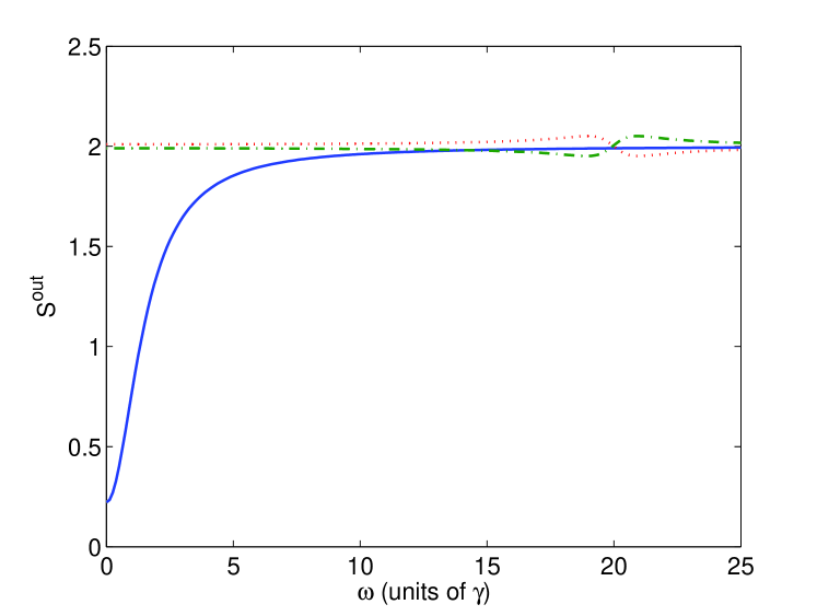
Figure 4: Output spectral variances of the combined modes for $J_{b}=\Delta_{b}=\gamma_{a}=\gamma_{b}=\gamma=1$ and $J_{a}=\Delta_{a}=10$. The solid line is $S_{Y_{p}}^{\text{out}}$, the dash-dotted line is $S_{X_{m}}^{\text{out}}$, and the dotted line is $S_{Y_{m}}^{\text{out}}$. A value of less than $2$ represents squeezing. The pump amplitude is $\epsilon=0.5\epsilon_{c}$.

Using these results, we can now investigate the degree of entanglement, as done above for the resonant case. As shown in Fig. 5, we find that the quadratures $Y_{p}$ and $X_{m}$ are entangled, exactly as in the single OPO case. As with the squeezing, the detunings have moved the maximum of entanglement to zero frequency. A sign of the out of resonance mode attempting to resonate is seen in the small degree of entanglement apparent around $\omega\approx 20\gamma$. We also see that the degree of entanglement is less than in the case with zero detuning, shown previously in Fig. 2, although it must be remembered that the absolute pump powers are not the same, merely the ratios $\epsilon/\epsilon_{c}$. Finding analytical expressions for EPR correlations is not possible using this coupled-mode approach, as, although we can calculate the necessary covariances, for example, $V(\hat{X}_{1},\hat{X}_{2})=[V(X_{p})-V(X_{m}))]/4$, it is not obvious how to separate out the single-mode variances. However, these can still be calculated numerically using the full single-mode equations with the appropriate detunings. That the system clearly demonstrates the EPR paradox is shown in Fig. 6, although again the maximum inferred violation is less than in the resonant case.

We note here that all the quantities shown for the detuned system are actually calculated at a lower absolute pump power than in the resonant case. For positive detunings, the critical pump amplitude is found as

$$\epsilon_{c}=\sqrt{[\gamma_{a}^{2}+(J_{a}-\Delta_{a})^{2}][\gamma_{b}^{2}+(J_{b}-\Delta_{b})^{2}]}/\kappa\,\,,$$ (45)

so that our choice of detunings means this is no longer a function of the coupling strengths. Therefore a careful choice of detunings has two main advantages in that it fixes the quadratures for which the maxima of quantum features are found, and means that the pumping necessary to a good performance does not vary with the coupling strengths.

The choice of detunings shown has the possible disadvantage that, as the effective coupling is now only in the $A_{m}$ mode, which is moved away from resonance, the quantum correlations which depend on both the modes are slightly degraded. This is readily seen from the figures because those correlations which include $X_{m}$ and $Y_{m}$ change more with $J_{a}$ than do the others.

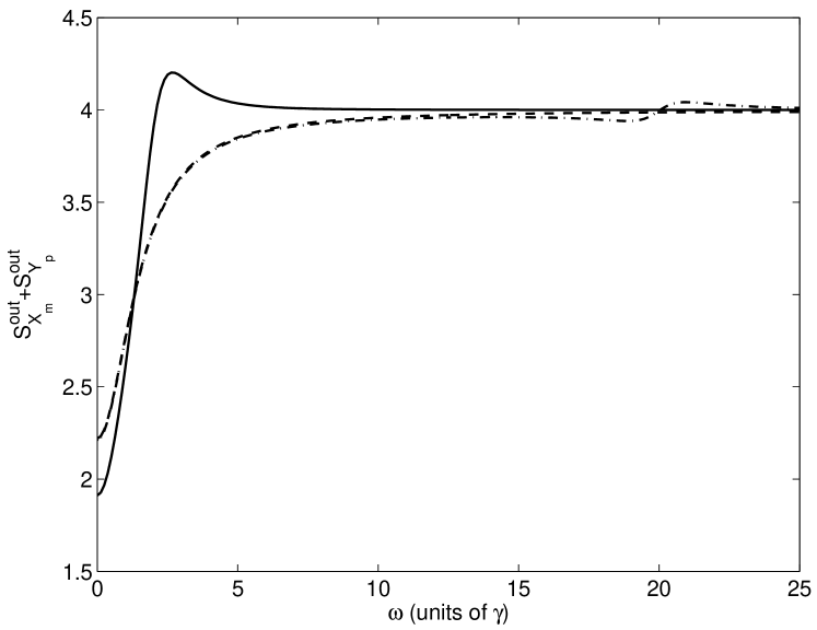
Figure 5: The sum of the output spectral variances, $S_{X_{m}}^{\text{out}}+S_{Y_{p}}^{\text{out}}$, for $J_{b}=\Delta_{b}=\gamma_{a}=\gamma_{b}=\gamma=1$ and $J_{a}=\Delta_{a}=1$ (solid line), $10$ (dash-dotted line) and $20$ (dashed line). A value of less than $4$ represents entanglement. The pump amplitude is $\epsilon=0.5\epsilon_{c}$.

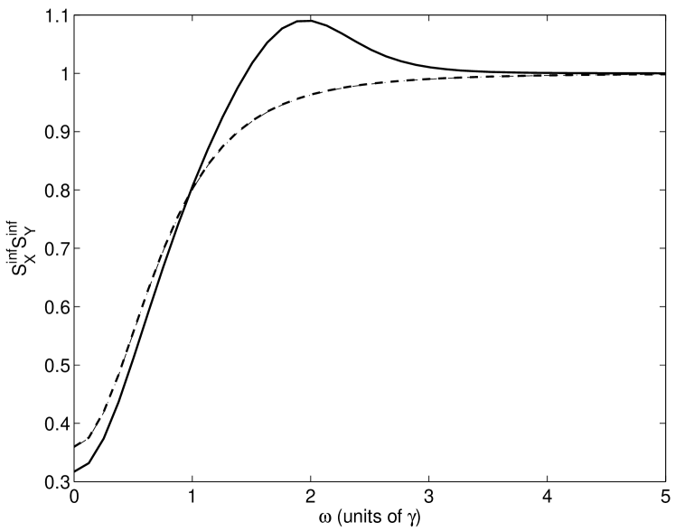
Figure 6: The product of the inferred output spectral variances, $S_{X}^{inf}S_{Y}^{inf}$, for $J_{b}=\Delta_{b}=\gamma_{a}=\gamma_{b}=\gamma=1$ and $J_{a}=\Delta_{a}=1$ (solid line) and $10$ (dash-dotted line). On this scale, the result for $J_{a}=20$ is indistinguishable from that for $J_{a}=10$. A value of less than $1$ represents a demonstration of the EPR paradox. The pump amplitude is $\epsilon=0.5\epsilon_{c}$.

VI Conclusion

This system exhibits a wide range of behaviour and is potentially an easily tunable source of single-mode squeezing, entangled states and states which exhibit the EPR paradox. The spatial separation of the output modes means that they do not have to be separated by optical devices before measurements can be made, along with the unavoidable losses which would result from this procedure. The entangled beams produced can be degenerate in both frequency and polarisation, unlike those of the nondegenerate OPO, and would exit the cavity at spatially separated locations. This may be a real operational advantage over the nondegenerate OPO, which is also known to produce nonclassical states. The tunability that exists because of the number of different parameters which can be experimentally accessed, such as the coupling strength, the pump intensity and the detunings, may make it interesting for a range of potential applications which would require the availability of states of the electromagnetic field with varying degrees of nonclassicality. Since this type of system is compatible with integrated optics techniques, it may provide a more robust source of entanglement than interferometers that use discrete optical components.

- (1) A. Einstein, B. Podolsky, and N. Rosen, Phys. Rev. 47, 777, (1935).
- (2) M.D. Reid and P.D. Drummond, Phys. Rev. Lett. 60, 2731, (1988); P. Grangier, M.J. Potasek and B. Yurke, Phys. Rev. A38, 3132, (1988); B.J. Oliver and C.R. Stroud, Phys. Lett. A 135, 407, (1989).
- (3) M.D. Reid, Phys. Rev. A40, 913 (1989).
- (4) M.D. Reid and P.D. Drummond, Phys. Rev. A40, 4493 (1989), P.D. Drummond and M.D. Reid, Phys. Rev. A41, 3930 (1990).
- (5) Z.Y. Ou, S.F. Pereira, H.J. Kimble, and K.C. Peng, Phys. Rev. Lett. 68, 3663, (1992).
- (6) J. Per̆ina, Jr. and J. Per̆ina, in Progress in Optics,, edited by E. Wolf (Elsevier, Amsterdam, 2000).
- (7) A.-B.M.A. Ibrahim, B.A. Umarov, and M.R.B. Wahiddin, Phys. Rev. A61, 043804, (2000).
- (8) S.A. Podoshvedov, J. Noh, and K. Kim, Opt. Commun. 212, 115, (2002).
- (9) L. Mis̆ta Jr, J. Herec, V. Jelínek, J. R̆ehác̆ek, and J. Per̆ina, J. Opt. B: Quant. Semiclass. Opt. 2, 726, (2000).
- (10) J. Herec, J. Fiurás̆ek, and L. Mis̆ta Jr., J. Opt. B: Quant. Semiclass. Opt. 5, 419, (2003).
- (11) M. Bache, Yu.B. Gaididei and P.L. Christiansen, Phys. Rev. A67, 043802, (2003).
- (12) M. Martinelli, C.L.G. Alzar, P.H.S. Ribeiro, and P. Nussenzveig, Braz. J. Phys. 31, 597, (2001).
- (13) L. Longchambon, J. Laurat, T. Coudreau, and C. Fabre, Eur. Phys. J. D 30, 279, (2004).
- (14) L. Longchambon, J. Laurat, T. Coudreau, and C. Fabre, Eur. Phys. J. D 30, 287, (2004).
- (15) C.W. Gardiner, Quantum Noise, (Springer-Verlag, Berlin, 1991).
- (16) R.J. Glauber, Phys. Rev. 131, 2766, (1963).
- (17) E.C.G. Sudarshan, Phys. Rev. Lett. 10, 277, (1963).
- (18) P.D. Drummond and C.W. Gardiner, J. Phys. A 13, 2353, (1980).
- (19) D.F. Walls and G.J. Milburn, Quantum Optics, (Springer-Verlag, Berlin, 1995).
- (20) C.W. Gardiner and M.J. Collett, Phys. Rev. A31, 3761, (1985).
- (21) C.W. Gardiner, Handbook of Stochastic Methods, (Springer-Verlag, Berlin, 1985).
- (22) M.J. Collett and C.W. Gardiner, Phys. Rev. 30, 1386, (1984).
- (23) M.K. Olsen, S.C.G. Granja, and R.J. Horowicz, Opt. Commun. 165, 293, (1999).
- (24) K. Dechoum, P.D. Drummond, S. Chaturvedi, and M.D. Reid, Phys. Rev. A70, 053807, (2004).
- (25) L.-M. Duan, G. Giedke, J.I. Cirac, and P. Zoller, Phys. Rev. Lett. 84, 2722, (2000).
- (26) C.M. Caves, Phys. Rev. D26, 1817, (1982).
- (27) C.M. Caves and B.L. Schumaker, Phys. Rev. A31, 3068, (1985).