Engineering mixed states in a degenerate four-state system

Abstract

A method is proposed for preparing any pure and a wide class of mixed quantum states in the decoherence-free ground-state subspace of a degenerate multilevel lambda system. The scheme is a combination of optical pumping and a series of coherent excitation processes, and for a given pulse sequence the same final state is obtained regardless of the initial state of the system. The method is robust with respect to the fluctuation of the pulse areas, like in adiabatic methods, however, the field amplitude can be adjusted in a larger range.

Controlling the quantum state of degenerate quantum systems have drown much attention recently. This field has developed independently in several different series of studies: Among the numerous adiabatic passage techniques Vitanov01 one of the most well-known method is the stimulated Raman adiabatic passage (STIRAP) AAMOP . The STIRAP can be used not only for transferring population between two quantum states using crafted laser pulses, but it has been utilized to create coherent superpositions in three- and four-level systems Marte91 ; Unanyan98 ; Theuer99 , to prepare maximally coherent superposition states Unanyan01 and arbitrary coherent superpositions Kis01 ; Kis02 ; Kis03 in $N$-state degenerate systems. The applicability of the STIRAP method is limited by constraints on the field amplitudes AAMOP ; Vitanov97 .

The other field that developed toward the quantum control of degenerate systems is termed “coherent control” that uses several interfering pathways in the quantum system to transfer selectively population from an initial state to a target one Shapiro03 . Merging this technique with the STIRAP method led to the mapping of wave-packets between vibrational potential surfaces in molecules for the non-degenerate Kraal02a and degenerate Thanopulos04 ; Gong04 cases.

The above mentioned control processes have great importance in many areas of quantum-information processing (QIP), involving quantum computing, cryptography and teleportation Nielsen00 . In general, mixed states cannot be created with coherent state preparation methods. However, for several QIP problems it is essential to develop quantum state preparation techniques which are capable to prepare not only pure, but mixed states of the system as well Bacon01 ; Somma02 ; Tarasov02 .

In optical pumping processes pump , the final state of the system is largely independent of its initial state, however, the efficiency is small Shore90 . On the other hand, in the coherent state-preparation methods the final state depends on the initial state of the system, but the efficiency can be nearly unity Vitanov01 ; AAMOP . In this letter we consider a novel concept for quantum-state preparation, which is a combination of optical pumping and coherent excitation processes, exhibiting only the advantageous properties of the two schemes, and capable to prepare not only pure but prescribed mixed states of the system too. The unique features of our method compared to other state-preparation methods are the following: it is simultaneously (i) robust, (ii) the final state is independent of the initial state of the system, (iii) the state is prepared in a decoherence-free subspace, (iv) the choice of the excitation field amplitude is quite arbitrary. The method can be implemented in multilevel lambda systems. For concreteness, let us consider the four-state system shown in Fig. 1: there are three degenerate ground states and a single excited state coupled by an elliptically polarized coherent laser pulse. The ground states $|g_{q}\rangle$ $(q=-,\pi,+)$ are assumed to be the magnetic sublevels of a $J_{g}=1$ angular momentum state, whereas the excited state $|e\rangle$ has $J_{e}=0$. The three polarization components of the coupling field, denoted by ${\cal E}_{q}$ with $(q=-,\pi,+)$, share the same time-dependence, but they can have different peak amplitudes and phases

$${\cal E}_{-}(t) = {\cal E}(t)\,e^{i\xi}e^{i\mu_{-}}\sin\theta\sin\varphi\,,$$ (1a)

$${\cal E}_{\pi}(t) = {\cal E}(t)e^{i\xi}\cos\theta\,,$$ (1b)

$${\cal E}_{+}(t) = {\cal E}(t)\,e^{i\xi}e^{i\mu_{+}}\sin\theta\cos\varphi\,,$$ (1c)

where the parameters $\theta$, $\varphi$ describe the polarization of the pulses, $\xi$ is the absolute phase of the pulse, and the phases of the $\sigma_{+}$ and $\sigma_{-}$ components relative to the $\pi$ component are $\mu_{+}$ and $\mu_{-}$, respectively. The excited state $|e\rangle$ decays with spontaneous emission to the ground states with a rate of $\gamma_{\textrm{in}}$, and it may decay to states other than the three ground states with a rate of $\gamma_{\textrm{ext}}$ as well. When decay out of the ground-state space occurs, a repumping process with a rate of $R_{p}$ is switched on in order to compensate for the population loss. We show that by using a predetermined sequence of pulses we can create any prescribed pure or a wide class of mixed final states in the ground-state space, starting from any initial state.

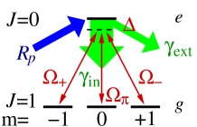
Figure 1: (Color Online) The coupling scheme for our state-engineering procedure: the lower states are the magnetic sublevels of a $J=1$ angular momentum state which are coupled by $\sigma_{\pm}$ and $\pi$ polarized pulses to a single excited state. The excited state decays with a rate $\gamma_{\rm in}$ into the lower states, and it may decay out of the system with a rate $\gamma_{\rm ext}$. For non-zero $\gamma_{\rm ext}$ a repumping is switched on with a rate $R_{p}$.

The Master equation describing the time evolution of the system is given by

$$\frac{\mathrm{d}}{\mathrm{d}t}\widehat{\varrho} = \frac{1}{i\hbar}[\widehat{H},\widehat{\varrho}]$$

$$+ \frac{\gamma_{\mathrm{in}}}{2}\sum_{l=-,\pi,+}2\widehat{L}_{l}^{\phantom{\dagger}}\widehat{\varrho}\widehat{L}_{l}^{\dagger}-\widehat{L}_{l}^{\dagger}\widehat{L}_{l}^{\phantom{\dagger}}\widehat{\varrho}-\widehat{\varrho}\widehat{L}_{l}^{\dagger}\widehat{L}_{l}^{\phantom{\dagger}}$$

$$- \frac{\gamma_{\textrm{ext}}}{2}\widehat{L}_{e}\widehat{\varrho}-\frac{\gamma_{\textrm{ext}}}{2}\widehat{\varrho}\widehat{L}_{e}+R_{p}(1-{\mathrm{T}r}\left\{\widehat{\varrho}\right\})\widehat{L}_{e},$$

where the Hamiltonian $\widehat{H}$ reads

$$\widehat{H} = \frac{\hbar}{2}(\Omega_{-}|g_{-}\rangle\langle e|\,+\,\Omega_{\pi}|g_{\pi}\rangle\langle e|\,+\,\Omega_{+}|g_{+}\rangle\langle e|+\textrm{h.c.})$$ (3)

$$+ \hbar\Delta|e\rangle\langle e|\,,$$

where the Rabi frequencies are $\Omega_{-}=\frac{1}{3}\Omega e^{i\xi}e^{i\mu_{-}}\sin\theta\sin\varphi$, $\Omega_{\pi}=-\frac{1}{3}\Omega e^{i\xi}\cos\theta$, $\Omega_{+}=\frac{1}{3}\Omega e^{i\xi}e^{i\mu_{+}}\sin\theta\cos\varphi$, with $\hbar\Omega=d_{ge}{\cal E}$. The step operators are defined as $\widehat{L}_{q}=\frac{1}{\sqrt{3}}|g_{q}\rangle\langle e|$ and $\widehat{L}_{e}=|e\rangle\langle e|$. The other symbols are defined above.

The Hamiltonian of Eq. (3) has two uncoupled eigenstates $|\Phi_{D}^{(l)}\rangle$ Morris83 , i.e. they are decoupled from the external driving field, $\widehat{H}|\Phi_{D}^{(l)}\rangle=0$ for $l=1,2$. They read

$$|\Phi_{D}^{(l)}\rangle=\sum_{q=-,\pi,+}n_{q}^{(l)}|g_{q}\rangle\,,\quad l=1,2\,,$$ (4)

where the unit vectors ${\bm{n}}^{(l)}$ are given by ${\bm{n}}^{(1)}=[e^{i\mu_{-}}\cos\theta\sin\varphi,\sin\theta,e^{i\mu_{+}}\cos\theta\cos\varphi]^{T}$ and ${\bm{n}}^{(2)}=[-e^{-i\mu_{+}}\cos\varphi,0,e^{-i\mu_{-}}\sin\varphi]^{T}$, and the field parameters $\mu_{\pm}$, $\varphi$, $\theta$ are defined in Eq. (1). These states are dark states, because they do not have a component in the excited state Arimondo96 . The Hamiltonian has two other eigenstates with non-zero eigenvalues, they are called bright states, because they do have a component in the excited state Arimondo96 .

Let us assume that we have some initial state $\widehat{\varrho}_{\textrm{in}}$ defined in the decoherence-free, ground-state space. The Hamiltonian part of the Master equation (Engineering mixed states in a degenerate four-state system) drives the bright components of this state to the excited state back and forth via Rabi oscillations. As the excited state gets populated the spontaneous emission will interrupt the Hamiltonian dynamics and the system falls back into the ground-state space or some other external states become populated. As a result, the two dark states become more and more populated, even though they are decoupled from the external driving field. When there is no decay into external states or the decay out of the four-state system is compensated by an incoherent repumping process, the system will relax into the dark subspace of the Hamiltonian. Then, the state of the system is given by

$$\widehat{\varrho}_{\textrm{out}}=p^{(1)}|\Phi_{D}^{(1)}\rangle\langle\Phi_{D}^{(1)}|+p^{(2)}|\Phi_{D}^{(2)}\rangle\langle\Phi_{D}^{(2)}|\,,$$ (5)

where the coefficients $p^{(l)}$ depend on the applied pulse and the initial state as well. It is important to note that this output state is independent of the pulse amplitude $\cal E$, it depends only on the polarization and relative phases of the three components of the field of Eq. (1).

In the ground-state space the state $|\Phi^{(\perp)}\rangle$ orthogonal to the dark states of Eq. (4) is $|\Phi^{(\perp)}\rangle=e^{i\mu_{-}}\sin\theta\sin\varphi\,|g_{-}\rangle-\cos\theta\,|g_{\pi}\rangle+e^{i\mu_{+}}\sin\theta\cos\varphi\,|g_{+}\rangle$ . This vector can point to anywhere in the three-dimensional ground-state space, depending on the laser-field parameters. Consequently, it is possible to choose the laser-field parameters, so that any two linearly independent state vectors $|\psi_{1}\rangle$ and $|\psi_{2}\rangle$ of the three-dimensional ground-state space lay in the dark subspace. Therefore, in principle there exists a pulse-sequence, such that any prescribed final state of the form

$$\widehat{\varrho}_{\textrm{f}}=p_{\textrm{f}}^{(1)}|\psi_{1}\rangle\langle\psi_{1}|+p_{\textrm{f}}^{(2)}|\psi_{2}\rangle\langle\psi_{2}|\,,$$ (6)

can be obtained. The state $\widehat{\varrho}_{\textrm{f}}$ can be either a pure state if one of the coefficients $p_{\textrm{f}}^{(l)}$ vanishes, or a mixed state if both of them are non-zero.

We have two tasks now: (i) to find how an initial state $\widehat{\varrho}_{\textrm{in}}$ transforms when the pulses Eq. (1) are adjusted to a certain value; (ii) to find the pulse-sequence that steer the state of the system to a prescribed final state defined by Eq. (6).

For convenience, the linear space of the density operators $\{\widehat{\varrho}\}$ is represented by vectors $\{{\bm{r}}\}$ with components $r_{4(i\smash{-}1)\smash{+}j}=(\widehat{\varrho})_{i,j}$, where $(\widehat{\varrho})_{i,j}$ is the matrix element of the density operator $\widehat{\varrho}$ in the ordered basis $\{|g_{-}\rangle,|g_{\pi}\rangle,|g_{+}\rangle,|e\rangle\}$ . The scalar product of vectors is defined as $({\bm{r}}^{(1)}|{\bm{r}}^{(2)})=\sum_{s}{r^{(1)*}_{s}}r^{(2)}_{s}={\rm Tr}\left\{\widehat{\varrho}^{(1)}\widehat{\varrho}^{(2)}\right\}$. The Master equation (Engineering mixed states in a degenerate four-state system) in this representation takes the form $\frac{\mathrm{d}}{\mathrm{d}t}\bm{r}=\bm{M}\bm{r}+\bm{d}$, where the matrix ${\bm{M}}$ describes the linear part of the Master equation (Engineering mixed states in a degenerate four-state system), and ${\bm{d}}$ corresponds to the constant term $R_{p}\widehat{L}_{e}$ in the incoherent repumping of the excited state. In this letter we are going to consider two cases:

($\alpha$) The case $\gamma_{\textrm{ext}}=R_{p}=0$ : In this case the Master equation is homogeneous in $\bm{r}$, and $\bm{d}$ is zero. The relaxation of the system into its final state can be described by those left- and right-hand eigenvectors (denoted by ${\bm{r}}_{\rm L}^{(k)}$ and ${\bm{r}}_{\rm R}^{(k)}$, respectively) of the matrix $\bm{M}$, which belong to the eigenvalue zero

$$\bm{M}\bm{r}^{(k)}_{\rm R}=\bm{0}\,,\quad{\bm{r}^{(k)\,T}_{\rm L}}\bm{M}=\bm{0}\,,$$ (7)

and are orthonormal $(\bm{r}^{(k)}_{\rm L}|\bm{r}^{(l)}_{\rm R})=\delta_{kl}$. The left- and right-hand zero subspaces of ${\bm{M}}$ are four-dimensional and they are different. The density matrices corresponding to the right-hand eigenstates ${\bm{r}}_{\textrm{R}}^{(k)}$ are composed from the dark eigenstates $|\Phi_{D}^{(l)}\rangle$ of the Hamiltonian (3), as

$$\widehat{\varrho}^{(1)}_{\rm R} = \frac{1}{\sqrt{2}}\left(|\Phi_{D}^{(1)}\rangle\langle\Phi_{D}^{(1)}|-|\Phi_{D}^{(2)}\rangle\langle\Phi_{D}^{(2)}|\right)\,,$$ (8a)

$$\widehat{\varrho}^{(2)}_{\rm R} = \frac{1}{\sqrt{2}}\left(|\Phi_{D}^{(1)}\rangle\langle\Phi_{D}^{(2)}|+|\Phi_{D}^{(2)}\rangle\langle\Phi_{D}^{(1)}|\right)\,,$$ (8b)

$$\widehat{\varrho}^{(3)}_{\rm R} = \frac{i}{\sqrt{2}}\left(|\Phi_{D}^{(2)}\rangle\langle\Phi_{D}^{(1)}|-|\Phi_{D}^{(1)}\rangle\langle\Phi_{D}^{(2)}|\right)\,,$$ (8c)

$$\widehat{\varrho}^{(4)}_{\rm R} = \frac{1}{\sqrt{2}}\left(|\Phi_{D}^{(1)}\rangle\langle\Phi_{D}^{(1)}|+|\Phi_{D}^{(2)}\rangle\langle\Phi_{D}^{(2)}|\right)\,.$$ (8d)

As for the density matrix representation of the left-hand eigenstates ${\bm{r}}_{\textrm{L}}^{(k)}$, the first three $\widehat{\varrho}^{(k)}_{\rm L}$ are given by Eqs. (8a) – (8c), and tho fourth one is $\widehat{\varrho}^{(4)}_{\rm L}=\frac{1}{\sqrt{2}}\hat{I}$. The final state of the system, after the relaxation has finished, is given by ${\bm{r}}_{\rm out}=\sum_{k=1}^{4}(\bm{r}^{(k)}_{\rm L}|\bm{r}_{\rm in}){\bm{r}}^{(k)}_{\rm R}$ since in this state $\frac{\mathrm{d}}{\mathrm{d}t}{\bm{r}}_{\textrm{out}}=\bm{0}$. By using the density operator representation Eq. (8) of the eigenvectors ${\bm{r}}^{(k)}_{\rm L/R}$ of $\bm{M}$, the input-output transformation can be written in a simple form as $\widehat{\varrho}_{\mathrm{out}}={\cal T}_{a}(\widehat{\varrho}_{\mathrm{in}})$, where ${\cal T}_{a}(\widehat{\varrho})$ reads

$${\cal T}_{a}(\widehat{\varrho})=\widehat{\varrho}^{\prime}+\frac{1}{2}(1-{\rm Tr}\left\{\widehat{\varrho}^{\prime}\right\})\widehat{P}_{D}\,,\quad\widehat{\varrho}^{\prime}=\widehat{P}_{D}\widehat{\varrho}\widehat{P}_{D}$$ (9)

where $\widehat{P}_{D}$ is a projector into the dark subspace of the Hamiltonian (3), $\widehat{P}_{D}=\sum_{k=1}^{2}|\Phi_{D}^{(k)}\rangle\langle\Phi_{D}^{(k)}|$ .

$(\beta)$  The case $R_{p},\gamma_{\textrm{ext}}>0$: Now the excited state is repumped from all external decay channels incoherently with a rate of $R_{p}$. The linear differential equation that governs the time evolution of the density operator takes the form $\frac{\mathrm{d}}{\mathrm{d}t}({\bm{r}}-\widetilde{\bm{r}})={\bm{M}}^{\prime}({\bm{r}}-\widetilde{\bm{r}})$, where the constant vector $\widetilde{\bm{r}}$ satisfies ${\bm{M}}^{\prime}\widetilde{\bm{r}}=-\bm{d}$, and the density matrix corresponding to $\widetilde{\bm{r}}$ is

$$\widehat{\widetilde{\varrho}} = \sin^{2}\varphi|g_{+}\rangle\langle g_{+}|\,+\,\cos^{2}\varphi|g_{-}\rangle\langle g_{-}|$$ (10)

$$- \frac{1}{2}(e^{i(\mu_{+}-\mu_{-})}\sin 2\varphi|g_{+}\rangle\langle g_{-}|\,+\,\textrm{ h.c.})\,.$$

The left- and right-hand zero-subspaces of the matrix ${\bm{M}}^{\prime}$ coincide and they are three-dimensional. The eigenvectors ${\bm{r}}^{(i)}$, ($i=1,2,3$) satisfy the equation ${\bm{M}}^{\prime}({\bm{r}}^{(i)}-\widetilde{\bm{r}})=\bm{0}$, and the corresponding density matrices are given by Eqs. (8a)–(8c). Instead of the mapping in the case ($\alpha$), the input-output states are connected through the relation $\bm{r}_{\rm out}=\widetilde{\bm{r}}+\sum_{i=1}^{3}(\bm{r}^{(i)}|\bm{r}_{\rm in}-\widetilde{\bm{r}})\bm{r}^{(i)},$ which in the density matrix representation reads $\widehat{\varrho}_{\mathrm{out}}={\cal T}_{b}(\widehat{\varrho}_{\mathrm{in}})$, where ${\cal T}_{b}(\widehat{\varrho})$ is defined as

$${\cal T}_{b}(\widehat{\varrho})=\widehat{\widetilde{\varrho}}-\widehat{\widetilde{\varrho}}^{\prime}+\widehat{\varrho}^{\prime}+\frac{1}{2}(1-{\rm Tr}\left\{\widehat{\varrho}^{\prime}\right\})\widehat{P}_{D}\,,$$ (11)

where the prime denotes projection into the dark subspace as in Eq. (9).

Now we turn our attention to finding a pulse sequence that yields a desired final density operator of the form Eq. (6). The transformation of an initial density operator is described by the subsequent applications of the mappings of Eqs. (9) or (11)

$$\widehat{\overline{\varrho}}_{\rm f}={\cal T}^{(N)}(\,{\cal T}^{(N-1)}(\ldots{\cal T}^{(1)}(\widehat{\rho}_{\rm i})\ldots))\,,$$ (12)

where ${\cal T}(\widehat{\varrho})$ is equal to ${\cal T}_{a}(\widehat{\varrho})$ or ${\cal T}_{b}(\widehat{\varrho})$. We have to choose the number of steps $N$, then to find the relative pulse amplitudes and phases, defined in Eq. (1), by means of minimizing numerically the functional

$${\cal J}(\{{\cal{E}}\},\widehat{\varrho}_{\rm in},\widehat{\varrho}_{\rm f})=\left(1-{\rm Tr}\{\widehat{\overline{\varrho}}_{\rm f}\widehat{\varrho}_{\rm f}\}\right)^{1/2}\,,$$ (13)

which is the mismatch between the obtained $\widehat{\overline{\varrho}}_{\rm f}$  (Eq. (12)) and the required $\widehat{\varrho}_{\rm f}$  (Eq. (6)) final density operators. The numerical optimization can be performed by means of e.g. the conjugate gradient method numrec . Due to the special linear property of the mappings ${\cal T}(p_{1}\widehat{\rho}_{1}+p_{2}\widehat{\rho}_{2})=p_{1}{\cal T}(\widehat{\rho}_{1})+p_{2}{\cal T}(\widehat{\rho}_{2})$ for $p_{1}+p_{2}=1$, it is sufficient to study the convergence for pure initial states, which are the arbitrary linear superpositions of the ground states. Our aim is to reach a prescribed destination density operator by applying the same fixed laser pulse sequence for all initial states.

Let us consider a concrete example to demonstrate the efficiency of the proposed state engineering method: We choose the destination density operator as

$$\widehat{\overline{\varrho}}_{\rm f}=\frac{1}{3}|\psi_{\rm f}^{(1)}\rangle\langle\psi_{\rm f}^{(1)}|+\frac{2}{3}|\psi_{\rm f}^{(2)}\rangle\langle\psi_{\rm f}^{(2)}|,$$ (14)

with two pure states

$$|\psi_{\rm f}^{(1)}\rangle=\left[\begin{array}[]{c}\frac{2}{7}e^{i\pi/3}\\[2.0pt] \frac{3}{7}e^{i\pi/5}\\[2.0pt] \frac{6}{7}\\[2.0pt] 0\end{array}\right]\,,\quad|\psi_{\rm f}^{(2)}\rangle=\left[\begin{array}[]{c}\frac{3}{5}\\[2.0pt] \frac{4}{5}e^{i\pi/7}\\[2.0pt] 0\\[2.0pt] 0\end{array}\right]\,.$$ (15)

First we discuss the case when $\gamma_{\rm ext}=R_{p}=0$: The initial set $\overline{\cal H}$ is obtained by discretizing the four-dimensional parameter space – two relative phases and two relative amplitudes – describing the possible pure initial states. Then we have taken a four-step excitation process, i.e. $N=4$ in Eq. (12), and used the conjugate gradient method to minimize the functional ${\cal J}(\{{\cal E}\},\widehat{\varrho}_{\rm in},\widehat{\varrho}_{\rm f})$ of Eq. (13) on the subset $\overline{\cal H}$, $\widehat{\varrho}_{\rm in}=|\psi_{\rm in}\rangle\langle\psi_{\rm in}|$ and $|\psi_{\rm in}\rangle\in\overline{\cal H}$. The outcome of the optimization is a sequence of four polarization angles and relative phases ($\varphi^{(l)},\theta^{(l)},\mu_{-}^{(l)},\mu_{+}^{(l)}$) for $l=1,\ldots,4$, which characterize the pulse sequence $\{{\cal E}\}$. This pulse sequence effects for any initial state such a final state, for which the mismatch Eq. (13) is less than $\approx 10^{-5}$ (limited by machine-precision). The subsequent stages of the transformation of the initial set $\overline{\cal H}$ are shown in Fig. 2. After the first pulse (Fig. 2a) the closure of the transformed initial set is the surface of the Bloch sphere. The second step (Fig. 2b) yields an elongated cigar-shape, while the third step an ellipsoid (Fig. 2c) distribution, finally the fourth step (Fig. 2d) contracts the distribution to a point-like region in the Bloch sphere with radius around $\approx 10^{-5}$. Then we solved numerically the Master equation (Engineering mixed states in a degenerate four-state system) inserting the obtained optimal pulse sequence, with a constant $\Omega=1$ and $\gamma_{\rm in}=1$. The pulse duration for each step should be chosen so that the relaxation process into the actual dark subspace terminates practically. These times can be estimated from the eigenvalues of the matrix $\bm{M}$: the one with the smallest absolute real part limits the speed of the convergence. We note that we have found convergence for any other prescribed final state as well, however, the required number of steps depends on the purity of the target state: the purer the state (i.e. $p_{\rm f}^{(1)}\ll p_{\rm f}^{(2)}$ or $p_{\rm f}^{(1)}\gg p_{\rm f}^{(2)}$ in Eq. (6) ), the larger the number of steps required.

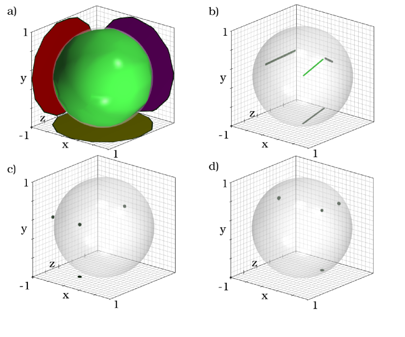
Figure 2: (Color Online) The transformation of the initial-state set after the first- (a), second- (b), third- (c), and fourth- (d) excitation steps, shown in the Bloch-sphere of the two-dimensional dark subspace. The coordinates are defined through the relation $\widehat{\varrho}=\frac{1}{2}(1+x\widehat{\sigma}_{x}+y\widehat{\sigma}_{y}+z\widehat{\sigma}_{z})$, where $\widehat{\sigma}_{q}$ are the Pauli’s spin operators. The projections of the distributions to the coordinate planes are also shown.

For non-zero $\gamma_{\rm ext}$ and $R_{p}$ the optimization of the pulse sequence can be done as in the previous case. In a four-step process, the numeric optimization yielded a pulse sequence for which the mismatch (Eq. (13)) is less than $\approx 10^{-5}$. We have found that the shape of the initial distribution transforms in the course of the subsequent stages of the excitation process in the same manner as before. Then we solved numerically the Master equation using the obtained optimal pulse sequence, setting the Rabi frequency $\Omega$, the decay constants $\gamma_{\rm in}$ and $\gamma_{\rm ext}$, and the repumping rate $R_{p}$ to unity: we have found that the process converges similarly to the previous case. We note that the ratios of $\gamma_{\rm in},\gamma_{\rm ext}$, and $R_{p}$ influence the rapidity of the convergence. For sufficiently long time steps the process always converges.

In summary we have worked out a scheme to create any pure or a wide class of mixed states in a four-state degenerate $\Lambda$ system. Our method is based on an excitation-relaxation process, that drives the state of the system into the dark subspace of the Hamiltonian that governs the dynamics without the decay processes. Although our method is not adiabatic, it is robust, because the final state is insensitive to the fluctuations in the pulse-area of the applied laser-field. A particular advantage of the method compared to the adiabatic schemes, that here we have a larger freedom to choose the field amplitude.

The authors acknowledge the support from the Research Fund of the Hungarian Academy of Sciences (OTKA) under contracts T043287 and T034484. ZK acknowledges the support from the János Bolyai program of the Hungarian Academy of Sciences.

References

(1) N.V. Vitanov, M. Fleischhauer, B.W. Shore, and K.
Bergmann, Adv. Atomic Mol. Opt. Phys. 46, 55 (2001).
(2) N.V. Vitanov, T. Halfmann, B.W. Shore, and K.
Bergmann, Ann. Rev. Phys. Chem. 52, 763 (2001).
(3) P. Marte, P. Zoller and J.L. Hall, Phys. Rev. A 44, R4118 (1991).
(4) R.G. Unanyan, M. Fleischhauer, B.W. Shore, and K.
Bergmann, Opt. Commun. 155, 144 (1998).
(5) H. Theuer, R.G. Unanyan, C. Habscheid, K. Klein,
and K. Bergmann, Opt. Express 4, 77 (1999).
(6) R.G. Unanyan, B.W. Shore, and K. Bergmann, Phys.
Rev. A 63, 043401 (2001).
(7) Z. Kis and S. Stenholm, Phys. Rev. A 64, 063406
(2001).
(8) Z. Kis and S. Stenholm, J. Mod. Optics 49, 111
(2002).
(9) A. Karpati and Z. Kis, J. Phys. B 36, 905
(2003).
(10) N.V. Vitanov and S. Stenholm, Phys. Rev. A 56, 1463 (1997).
(11) M. Shapiro and P. Brumer, Principles of the
Control of Molecular Processes, (Wiley-Interscience, 2003).
(12) P. Král, Z. Amitay, M. Shapiro, Phys. Rev. Lett.
89, 063002 (2002).
(13) I. Thanopulos, P. Král, and M. Shapiro, Phys.
Rev. Lett. 92, 113003 (2004).
(14) J. Gong and S.A. Rice, Phys. Rev. A 69, 063410
(2004).
(15) M.A. Nielsen, I.L. Chuang, Quantum Computation
and Quantum Information, (Cambridge University Press, Cambridge,
2000).
(16) R. Somma, G. Ortiz, J. E. Gubernatis, E. Knill, and
R. Laflamme, Phys. Rev. A 65, 042323 (2002).
(17) D. Bacon et al., Phys. Rev. A 64, 062302 (2001).
(18) V.E. Tarasov, J. Phys. A 35, 5207 (2002).
(19) A. Kastler, in Nobel Lectures, Physics 1963-1970, (Elsevier Publishing
Company, Amsterdam, 1972).
(20) B. W. Shore, The Theory of Coherent Atomic
Excitation, (Wiley, N.Y., 1990).
(21) J. R. Morris and B. W. Shore, Phys. Rev. A 27, 906 (1983).
(22) E. Arimondo, in Progress in Optics ed. E. Wolf,
vol. 35 (Elsevier, Amsterdam, 1996) p. 257.
(23) Press, W.H., Teukolsky, S.A., Vetterling, W.T.,
Flannery, B.P., 1997, Numerical Recipes in C, (Cambridge University
Press).