Stimulated Raman Adiabatic Passage (STIRAP) Among Degenerate-Level Manifolds

Abstract

We examine the conditions needed to accomplish stimulated Raman adiabatic passage (STIRAP) when the three levels ($g$, $e$ and $f$) are degenerate, with arbitrary couplings contributing to the pump-pulse interaction ($g$ - $e$) and to the Stokes-pulse interaction ($e$-$f$). We show that in general a sufficient condition for complete population removal from the $g$ set of degenerate states for arbitrary, pure or mixed, initial state is that the degeneracies should not decrease along the sequence $g$, $e$ and $f$. We show that when this condition holds it is possible to achieve the degenerate counterpart of conventional STIRAP, whereby adiabatic passage produces complete population transfer. Indeed, the system is equivalent to a set of independent three-state systems, in each of which a STIRAP procedure can be implemented. We describe a scheme of unitary transformations that produces this result. We also examine the cases when this degeneracy constraint does not hold, and show what can be accomplished in those cases. For example, for angular momentum states when the degeneracy of the $g$ and $f$ levels is less than that of the $e$ level we show how a special choice for the pulse polarizations and phases can produce complete removal of population from the $g$ set. Our scheme can be a powerful tool for coherent control in degenerate systems, because of its robustness when selective addressing of the states is not required or impossible. We illustrate the analysis with several analytically solvable examples, in which the degeneracies originate from angular momentum orientation, as expressed by magnetic sublevels.

I Introduction

Techniques based on adiabatic passage provide very practical methods for producing nearly complete transfer of population between two quantum states using crafted laser pulses Vitanov01 . One popular example of such coherent adiabatic excitation, stimulated Raman adiabatic passage (STIRAP) STIRAP , provides a simple and robust technique for transferring population between two nondegenerate metastable levels, making use of two pulses, termed the pump pulse (linking the initially populated ground state $\psi_{g}$ with excited state $\psi_{e}$) and the Stokes pulse (linking excited state $\psi_{e}$ with final state $\psi_{f}$ of the three-state chain). When the pulses are properly timed (Stokes preceding but overlapping the pump pulse) and two-photon resonance is maintained, then via adiabatic passage the population is transferred from initial to final state, without appreciable population in the excited state at any time.

The operation of STIRAP can be understood by introducing instantaneous eigenstates of the time-varying Hamiltonian, the time-dependent adiabatic states with associated time-dependent eigenvalues (adiabatic energies). One (and only one) of these states, $\Phi_{0}(t)$, is constructed from only the initial and final state, with no component of the excited state. Because the excited state generates fluorescence via spontaneous emission, such an adiabatic state will exhibit no such signal; it is termed a dark state. During the STIRAP process the state vector $\Psi(t)$ remains aligned with the adiabatic state $\Phi_{0}(t)$, while this state, in turn, changes composition from being aligned with $\psi_{g}$ initially to being aligned with $\psi_{f}$ after the Stokes-pump pulse sequence.

Numerous extensions of the basic three-state STIRAP STIRAP have been considered Vitanov01 ; AAMOP , including examples in which there occur magnetic sublevels and associated degeneracy. One possibility is that the atomic energy levels are coupled in such a way that each one is connected to at most two others. Population transfer in such multi-state chains has been studied by several authors Shore91 ; Smith92 ; Pillet93 ; Weiss94 ; Shore95 ; Martin95 ; Malinovsky97 ; Vitanov98 ; Theuer98 . In addition to straightforward population transfer, STIRAP has been applied to the problem of manipulating and creating coherent superpositions of two or more quantum states. Such superpositions are required for many contemporary applications including information processing and communication. The original STIRAP process has, for example, been utilized to create coherent superpositions in three- and four-level systems Marte91 ; Lawall94 ; Weitz94 ; Goldner94 ; Unanyan98 ; Theuer99 ; Unanyan99 and to prepare $N$-component maximally coherent superposition states Unanyan01 . There have been proposals to create $N$-component coherent superpositions in such systems, where the final state space is degenerate Kis01 ; Kis02 , at least in the rotating wave picture. This idea has been further developed to map wave-packets between vibrational potential surfaces in molecules Kraal02a ; Kraal02b . Finally, it has been shown for a specific degenerate system, having a single initial-, two degenerate intermediate-, and three degenerate final states coupled in the Raman configuration, that the STIRAP process can be extended to systems with degenerate intermediate and final levels Kis03 .

Yet an open question has remained: what is the most general system of three degenerate levels, linked via Raman process, for which it is possible to transfer all population from the ground-state manifold of degenerate states (the $g$ set) to the final-state manifold (the $f$ set) while minimizing population in the excited states (the $e$ set), without first using optical pumping to prepare a single nondegenerate initial state? We here provide the answer to this question.

We consider $N_{g}$ degenerate states of the $g$ set, coupled by means of a pump-pulse to $N_{e}$ degenerate states of the $e$ set, which in turn are linked by the Stokes pulse to $N_{f}$ degenerate states of the $f$ set. We will show that such a generalized STIRAP process is almost always possible if the succession of state-degeneracies is nondecreasing, i.e. $N_{g}\leq N_{e}\leq N_{f}$. When such conditions hold, then for arbitrary couplings among states (e.g. arbitrary elliptical polarization of electric dipole radiation between magnetic sublevels) it is possible to obtain complete adiabatic passage of all population from the states of the $g$ set into some combination of states of the $f$ set.

We also examine the possibility of adiabatic passage when this restriction on degeneracies does not hold. We show that in this case in general only part of the population can be transferred to the $f$ set. We point out that, in special but important cases, for an appropriate choice of the polarizations and phases of the coupling fields, a complete adiabatic population transfer can be obtained.

Another motivation of this paper is the creation of coherent superposition states in a degenerate system. The difficulty in such systems arises from the limited possibility of addressing a single preselected state: addressing of a selected state is usually achieved by exploiting selection rules that the coupling field should satisfy. However, if we have e.g. two Zeeman multiplets a light field with a certain polarization will create several couplings between the magnetic sublevels of the multiplets. Our scheme offers a solution to this problem: we show that despite of the lack of selective addressing of the degenerate states, we have some control over the created coherent superposition state in the $f$ set. As we point out, and illustrate with specific examples, the level of control depends on the system under consideration.

Our scheme is based on using a Morris-Shore (MS) transformation of the Stokes couplings or the pump couplings, thereby reducing this particular (generally complicated) linkage to a set of unlinked two-state systems and dark states Morris83 ; 5ss . Underlying this technique is the fact that, as Morris and Shore Morris83 have shown, any system of linkages in which there occur only two detunings (i.e. the system has two sets of degenerate sublevels, termed here $a$ and $b$, forming sets of dimension $N_{a}$ and $N_{b}$), can be transformed, via suitable redefinition of basis states, to one involving a set of $N_{<}$ independent two-state systems, where $N_{<}={\rm min}\{N_{a},N_{b}\}$, together with a set of uncoupled states that are unconnected to other states by the given couplings (one-state systems). If such an uncoupled state has no component from the $e$ set we term it a dark state. We here extend that work to produce sets of unlinked three-state systems.

The paper is organized as follows: In the next section we present a general model for degenerate, three-level systems and discuss its main properties. In Sec. III we derive a general condition for complete STIRAP-like population transfer. In Sec. IV we derive analytic expressions for the dark and bright states for important special choices of degeneracies. Then, in Sec. V, we determine the conditions needed for adiabatic evolution. We demonstrate our method through some specific examples in Sec. VI. Finally, in Sec. VII, we summarize our results.

II The Degenerate-Sublevel Model

II.1 The Hamiltonian

As is customary when dealing with STIRAP or other three-level chains, we introduce an expansion of the state vector $\Psi(t)$ that incorporates explicit phases taken from carrier frequencies of the pump and Stokes pulses, $\omega_{p}$ and $\omega_{S}$, respectively. In this rotating-wave picture, and with the customary neglect of counter-rotating terms [i.e. time variations $(\omega_{i}+\omega_{j})t$] the rotating-wave approximation (RWA) Hamiltonian takes the block-matrix form

$${\bm{H}}(t)=\left[\begin{array}[]{ccc}{\bm{0}}&p(t){\bm{P}}&{\bm{0}}\\ p(t){\bm{P}}^{\dagger}&\hbar{\bm{\Delta}}&s(t){\bm{S}}\\ {\bm{0}}&s(t){\bm{S}}^{\dagger}&{\bm{0}}\end{array}\right]\,,$$ (1)

for use with the Schrödinger equation

$$i\hbar\frac{d}{dt}{\bm{C}}(t)={\bm{H}}(t){\bm{C}}(t)\,.$$ (2)

Here the zeros ${\bm{0}}$ denote null square or rectangular matrices of appropriate dimensions. The zero matrix in the bottom right corner indicates that the system is supposed to maintain two-photon resonance. All time dependence occurs in the two pulse amplitudes $p(t)$ and $s(t)$, each with unit maximum value. The $N_{e}\times N_{e}$ diagonal matrix $\hbar\bm{\Delta}$ describes the detuning of the pump carrier frequency from the Bohr frequency of the $g-e$ transition. The $N_{g}\times N_{e}$ matrix $2p(t){\bm{P}}/\hbar$ consists of Rabi frequencies associated with the transitions between the $g$ and $e$ sets, $\hbar\Omega_{ij}(t)=2p(t)P_{ij}$. The elements of the constant matrix ${\bm{P}}$ read

$$P_{ij}=\frac{1}{2}{\cal E}^{(p)}\mu_{ij}\,,\qquad\left\{\begin{array}[]{l}i=1\cdots N_{g}\\ j=1\cdots N_{e}\end{array}\right.\,,$$ (3)

where ${\cal E}^{(p)}$ is the peak amplitude of the pump-pulse electric field and $\mu_{ij}$ is the dipole-transition moment.

Similarly, the $N_{e}\times N_{f}$ matrix $2s(t){\bm{S}}/\hbar$ consists of Rabi frequencies associated with the transitions between the $e$ and $f$ sets of states. The elements of the constant matrix $\bm{S}$ are

$$S_{ij}=\frac{1}{2}{\cal E}^{(S)}\mu_{ij}\,,\qquad\left\{\begin{array}[]{l}i=1\cdots N_{e}\\ j=1\cdots N_{f}\end{array}\right.\,,$$ (4)

where ${\cal E}^{(S)}$ is the peak amplitude of the Stokes electric field.

The structure of the RWA Hamiltonian of Eq. (1) is similar to that of the conventional three-state STIRAP, in having all time dependence confined to two pulses $p(t)$ and $s(t)$, but instead of single ground, excited, and final states we have degenerate manifolds of sublevels, and hence we have matrices $p(t){\bm{P}}$, $s(t){\bm{S}}$, and ${\bm{\Delta}}$ where conventional STIRAP would have scalar elements. To illustrate these Fig. 1 shows the linkage patterns for the angular momentum sequence $J=2\leftrightarrow 3\leftrightarrow 4$. To simplify the drawings we show the energies of successive manifolds as increasing, such as would occur with a ladder scheme; the connections are the same as with the usual lambda couplings, in which the final sublevels have energies below the excited state.

Figure 1: (Color Online) An example for the degenerate STIRAP scheme: we have three Zeeman multiplets with $J_{g}=2$, $J_{e}=3$, $J_{f}=4$. The couplings are those of $\sigma_{\pm}$ polarized pulses. The pump and Stokes pulses are detuned from exact resonance with the excited-state by $\Delta$, but they maintain two-photon resonance between states $g$ and $f$. The system separates into two independent systems, indicated by solid and dashed lines.

Although we discuss situations in which the coupling matrices result from magnetic-sublevel degeneracy, all of our results apply quite generally, for any mathematical form of the dipole-moment matrices and consequently for any arbitrary structure of the constant matrices ${\bm{S}}$ and ${\bm{P}}$.

II.2 Dark states

There exist $N=N_{g}+N_{e}+N_{f}$ basis states for this system, and hence $N$ adiabatic states ${\bm{\Phi}}_{n}(t)$. We can immediately apply the MS transformation Morris83 , at each instant of time, by placing the $g$ and $f$ sets of states together into the MS $a$ set, and taking the $e$ set to be the MS $b$ set. If the $a$ set is larger than the $b$ set, there will be $N_{u}=N_{a}-N_{b}$ uncoupled states. None of these have any component from the $e$ set, and so they are all dark states. The number of dark states is thus $N_{D}=N_{g}+N_{f}-N_{e}$. In the conventional nondegenerate STIRAP AAMOP , for which $N=3$, the MS transformation gives one dark state and one bright state; for the tripod system, for which $N=4$, there are two dark states Unanyan98 ; Theuer99 . In the angular-momentum system of Fig. 1 there are $N_{D}=5+9-7=7$ dark states.

For conventional nondegenerate STIRAP the composition of the dark state changes with time, because the coupling matrices and the MS transformation change with time. However, it is possible to associate the (single) dark state initially with the nondegenerate ground state by applying the pulses in the counterintuitive order, i.e. Stokes pulse preceding pump pulse. When there is degeneracy, it is necessary to establish that the entire population of any pure initial state in the $g$ set is projected into the set of dark states and no population is left in bright states. This completeness of the dark states is at the heart of our question concerning the possibility of STIRAP with degeneracy.

III General condition for complete population transfer

One of our basic questions is whether, for a given linkage pattern, it is possible to empty completely the $g$ set for any arbitrary initial state, once we have fixed the pump and Stokes pulses.

It is easy to see that one necessary condition for complete removal of population from the ground manifold is that there should not be more sublevels in this manifold than there are in the excited state, i.e. we require $N_{g}\leq N_{e}$

To prove this assertion we employ a MS transformation Morris83 on the pump transitions that connect ground and excited states. This transformation introduces a new set of basis states in each of these manifolds, such that each sublevel from the $g$ set couples to at most one sublevel from the $e$ set. Were there are no Stokes couplings between $e$ and $f$ states, the dynamics could be described as a set of independent two-state systems, together with some single states (uncoupled states) that are not affected by the pump radiation. Given such a revision of the basis states, it is easy to see that if there are more ground states than excited states, $N_{g}>N_{e}$, then the dark states will be composed of $g$-states and some population will be trapped there. This will remain unaffected by the radiation; population cannot be removed from them using this particular linkage pattern.

Figure 2 illustrates this accounting procedure. The top frame (a) shows a general coupling scheme for the sequence $J=2\leftrightarrow 1\leftrightarrow 2$. The MS transformation on the $g-e$ pump transition produces the description shown in the bottom frame (b). In the $g$ set, with this transformed basis, there occur two sublevels that have no connection with any excited states. Population cannot be removed from these as long as the couplings are those shown in the top frame.

It is easy to see that, had there been more sublevels in the $e$ set, such that $N_{g}\leq N_{e}$, then every one of the transformed states from the $g$ set would be linked to some excited state, with consequent possibility for population removal. There will also be uncoupled states in the $e$ manifold but they are unpopulated and do not affect the population transfer.

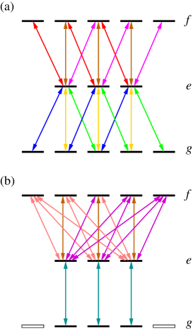
Figure 2: (Color Online) This sketch shows that when the number of ground-state-sublevels exceeds the number of excited-state-sublevels then it is impossible to transfer all the population from the ground-state manifold to the final-state manifold. Frame (a) shows the original coupling configuration. Frame (b) shows the couplings after a MS transformation on the $g-e$ transition. The empty rectangles represent uncoupled states. This transformation is independent of time, because all elements of the coupling share a common time dependence, $p(t)$. The presence of uncoupled sublevels in the $g$ set prevents removal of population from these states; hence it is not possible to remove all population from all of the ground-state sublevels.

The introduction of MS basis states in this way makes the $g-e$ linkage pattern quite simple, but by introducing a new basis the $e-f$ couplings become more complicated: generally there will be a connection between each transformed $e$ state and each (untransformed) $f$ state, as indicated in frame (b).

Next we consider the $e-f$ coupling. We can repeat the previous argument for the $g-e$ coupling with the replacements $g\leftrightarrow e$ and $e\leftrightarrow f$. We obtain, that the Stokes field MS transformation yields $N_{<}=\mbox{min}\{N_{e},N_{f}\}$ independent two level systems for the $e-f$ transition, plus $|N_{e}-N_{f}|$ uncoupled states in the larger one out of the $e$ and $f$ sets. It is easy to see that, had there been more sublevels in the $f$ set, such that $N_{e}\leq N_{f}$, then every one of the transformed states from the $e$ set would be linked to some final state, with consequent possibility for population removal. Combinig the arguments of the MS tarnsormations for the $g-e$ and $e-f$ couplings, we obtain that in general, if a non–descending sequence of state–degeneracies is fulfilled

$$N_{g}\leq N_{e}\leq N_{f}\,,$$ (5)

then a complete STIRAP-like population transfer from the $g$ set to the $f$ set is possible. We emphasize that in this case the success of the full transfer is independent of the initial state of the system: it can be any pure state or a mixed state as well.

A particularly important special case of degeneracy occurs when there are dark states but they are insufficient to produce complete population transfer. This occurs when $N_{g}+N_{f}>N_{e}$, but $N_{f}<N_{e}$. For example, in the linkage of $J=1\leftrightarrow 2\leftrightarrow 1$ there is 1 dark state. Figure 11 illustrates this situation.

IV The Stokes-field MS transformation

In this section we determine the dark states of the Hamiltonian of Eq. (1); these are the adiabatic states that will be utilized for the desired adiabatic population transfer. In order to simplify the structure of the Hamiltonian, we perform a MS transformation; here we take that to be on the $e-f$ couplings (those of the Stokes field). In our case the time-independent transformation matrix ${\bm{U}}$ is defined as

$${\bm{U}}=\left[\begin{array}[]{ccc}{\bm{I}}&{\bm{0}}&{\bm{0}}\\ {\bm{0}}&{\bm{B}}&{\bm{0}}\\ {\bm{0}}&{\bm{0}}&{\bm{A}}\end{array}\right]\,.$$ (6)

In the top-left corner there is a unit matrix ${\bm{I}}$ of dimension $N_{g}\times N_{g}$. This leaves the $g$ set of states unaltered. The $N_{f}\times N_{f}$ unitary matrix $\bm{A}$ transforms the sublevels in the final-state manifold. Similarly, the $N_{e}\times N_{e}$ unitary matrix $\bm{B}$ transforms the sublevels in the excited-state manifold. The constant matrices $\bm{A}$ and $\bm{B}$ are defined Morris83 such that by transforming the Hamiltonian Eq. (1) with the matrix $\bm{U}$ through the relation

$${\bm{U}}{\bm{H}}(t){\bm{U}}^{\dagger}=\left[\begin{array}[]{ccc}{\bm{0}}&p(t)\widetilde{\bm{P}}&{\bm{0}}\\ p(t)\widetilde{\bm{P}}^{\dagger}&\hbar{\bm{\Delta}}&s(t)\widetilde{\bm{S}}\\ {\bm{0}}&s(t)\widetilde{\bm{S}}^{\dagger}\end{array}\right]\,$$ (7)

we obtain a transformed pump-field coupling matrix $\widetilde{\bm{P}}={\bm{P}}{\bm{B}}^{\dagger}$, and a quasi-diagonal Stokes-field coupling matrix $\widetilde{\bm{S}}=\bm{B}\bm{S}\bm{A}^{\dagger}$. By quasi-diagonal we mean that the structure of the matrix is

$$\widetilde{\bm{S}}=\begin{cases}\left[\begin{array}[]{cc}\widetilde{\bm{\Sigma}}&{\bm{0}}\end{array}\right]&\mbox{ if }N_{f}>N_{e}\,,\\[6.0pt] \widetilde{\bm{\Sigma}}&\,\,\mbox{if }N_{f}=N_{e}\,,\\[2.0pt] \left[\begin{array}[]{c}\widetilde{\bm{\Sigma}}\\ {\bm{0}}\end{array}\right]&\mbox{ if }N_{f}<N_{e}\,,\end{cases}$$ (8)

where $\widetilde{\bm{\Sigma}}$ is a square diagonal matrix with dimension $N_{<}={\rm min}(N_{e},N_{f})$. The moduli of the diagonal elements are given by the square-roots of the common eigenvalues of the Hermitian matrices $\bm{S}\bm{S}^{{\dagger}}$ (of dimension $N_{e}\times N_{e}$) and $\bm{S}^{{\dagger}}\bm{S}$ (of dimension $N_{f}\times N_{f}$). The phases of the diagonal elements are obtained by evaluating directly the matrix product $\bm{B}\bm{S}\bm{A}^{\dagger}$. Some of the diagonal elements of $\widetilde{\bm{\Sigma}}$ might be zero, meaning that some $e-f$ couplings vanish in the MS basis. We here assume that in general all diagonal elements of $\widetilde{\bm{\Sigma}}$ are non-zero, i.e. it is nonsingular. We treat in Appendix B the case when this matrix is singular.

In the following subsections we consider the three important special cases of degeneracies and derive the adiabatic states of the coupled degenerate systems.

IV.1 The case $N_{g}\leq N_{e}\leq N_{f}$

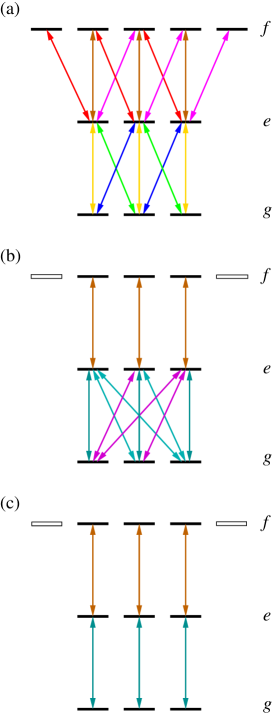
Figure 3: (Color Online) The three stages of the transformations. (a) The original coupling scheme. (b) The result of the Stokes-field MS transformation, converting the couplings between $e$ and $f$ sets into independent one- and two-state systems. (c) The result of redefining the states in the $g$, $e$, and $f$ sets.

We first consider the case when the MS transformation on the $e-f$ transition results in $N_{f}-N_{e}>0$ decoupled sublevels in the $f$ manifold. The coupling matrix $\widetilde{\bm{S}}$ takes the form given in the first row of Eq. (8), and hence the Hamiltonian in the MS basis reads

$$\widetilde{{\bm{H}}}(t)=\left[\begin{array}[]{cccc}{\bm{0}}&p(t)\widetilde{{\bm{P}}}&{\bm{0}}&{\bm{0}}\\ p(t)\widetilde{{\bm{P}}}^{\dagger}&\hbar{\bm{\Delta}}&s(t)\widetilde{\bm{\Sigma}}&{\bm{0}}\\ {\bm{0}}&s(t)\widetilde{\bm{\Sigma}}^{\dagger}&{\bm{0}}&{\bm{0}}\\ {\bm{0}}&{\bm{0}}&{\bm{0}}&{\bm{0}}\end{array}\right]\,.$$ (9)

As with the original RWA Hamiltonian, the only time dependence enters through the pulses $p(t)$ and $s(t)$.

We can treat the system in the same way when $N_{f}=N_{e}$. Then the coupling matrix $\widetilde{\bm{S}}$ is given by the second row of Eq. (8), and we have to omit all zero rows and columns from the Hamiltonian of Eq. (9). In either cases the sub-matrix $\widetilde{{\bm{P}}}$ has dimensions $N_{g}\times N_{e}$, while the square matrices $\widetilde{\bm{\Sigma}}$ and $\bm{\Delta}$ have dimensions $N_{e}\times N_{e}$.

To find the adiabatic eigenvectors $\widetilde{{\bm{\Phi}}}_{k}(t)$ of $\widetilde{{\bm{H}}}(t)$ we take their elements to have the form

$$\widetilde{{\bm{\Phi}}}_{k}(t)=\left[\begin{array}[]{c}{\bm{x}}_{k}(t)\\ \widetilde{\bm{y}}_{k}(t)\\ \widetilde{\bm{z}}_{k}(t)\\ \widetilde{\bm{z}}^{\prime}_{k}(t)\end{array}\right]\quad\begin{array}[]{c}{g}\\ {e}\\ {f}\\ {f^{\prime}}\end{array}$$ (10)

where $f^{\prime}$ denotes the subspace of uncoupled states in the $f$ set. Because these are unlinked to the $e$ set they meet the definition of dark states. Their population, if initially present, is preserved throughout the time evolution. When $N_{f}=N_{e}$ we simply omit the fourth row from this vector (the $f^{\prime}$ states), i.e. we do not have $\widetilde{\bm{z}}^{\prime}_{k}$. In Eq. (10) there is no tilde on the $x$ components because, unlike the $y$ and $z$ components, these do not transform in the Stokes field MS transformation. In Sec. IV B and C the $x$ components undergo a MS transformation, as is indicated there by a tilde.

The eigenvectors satisfy the eigenvalue equation

$$\widetilde{\bm{H}}(t)\widetilde{{\bm{\Phi}}}_{k}(t)=\varepsilon_{k}(t)\widetilde{{\bm{\Phi}}}_{k}(t)\,.$$ (11)

By substituting the Hamiltonian of Eq. (9) and the parameterization (10) of the eigenvectors into this equation we obtain four sets of coupled linear equations for ${\bm{x}}_{k}$, $\widetilde{\bm{y}}_{k}$, $\widetilde{\bm{z}}_{k}$, and $\widetilde{\bm{z}}^{\prime}_{k}$. The solution of these equations provide the dark and bright eigenvectors $\widetilde{{\bm{\Phi}}}_{k}(t)$ defined by Eq. (11).

Let us assume that there exists an eigenvalue zero, $\varepsilon_{0}=0$ . This is always possible to ensure, by suitable choice of the phases of the rotating wave approximation and the zero-point of energy. If we can find a solution of the eigenvalue-equation (11) for this case, then our assumption $\varepsilon_{0}=0$ holds, since the solution of the linear equations is unique. After some algebra one can obtain $N_{g}$ different vectors $\widetilde{{\bm{\Phi}}}^{(l)}_{0}(t)\,\,,l=1\ldots N_{g}$, that are linearly independent of each other, and can make these orthonormal

$$\widetilde{{\bm{\Phi}}}_{0}^{(l)}(t)={1\over{\cal N}_{0}^{(l)}(t)}\left[\begin{array}[]{c}s(t){\bm{x}}_{0}^{(l)}\\ {\bm{0}}\\ -p(t)\widetilde{\bm{\Sigma}}^{-1}\widetilde{{\bm{P}}}^{\dagger}{\bm{x}}_{0}^{(l)}\\ {\bm{0}}\end{array}\right]\,,$$ (12)

where ${\cal N}_{0}^{(l)}(t)$ is a (time dependent) normalization factor. Here we have assumed that the matrix $\widetilde{\bm{\Sigma}}$ is nonsingular. We will discuss separately, in Appendix B, the situation when $\widetilde{\bm{\Sigma}}$ is singular. Since the $y$ component of these vectors is zero, they have no component in the $e$ set; they correspond to dark states. To make the dark eigenvectors of Eq. (12) orthogonal we require that

$$s(t)^{2}\langle{\bm{x}}^{(k)\,T}_{0}|{\bm{x}}^{(l)}_{0}\rangle+p(t)^{2}\langle{\bm{x}}^{(k)\,T}_{0}|\widetilde{{\bm{P}}}\widetilde{\bm{\Sigma}}^{-1\dagger}\widetilde{\bm{\Sigma}}^{-1}\widetilde{{\bm{P}}}^{\dagger}|{\bm{x}}^{(l)}_{0}\rangle=0\,,$$ (13)

for $1\leq k<l\leq N_{g}$. The time-dependence of the envelope functions $s(t)$ and $p(t)$ is arbitrary, and therefore we require that the two terms on the left-hand-side (lhs) of Eq. (13) be identically zero. The eigenvectors of a Hermitian matrix can be chosen so that they are orthogonal to each-other, and therefore the first term on the lhs of Eq. (13) is automatically zero. It follows that the vectors ${\bm{x}}^{(l)}_{0}$ are the eigenvectors of the Hermitian matrix

$${\bm{M}}={\bm{P}}({\bm{S}}{\bm{S}}^{\dagger})^{-1}{\bm{P}}^{\dagger}\equiv\widetilde{{\bm{P}}}\widetilde{\bm{\Sigma}}^{-1\dagger}\widetilde{\bm{\Sigma}}^{-1}\widetilde{{\bm{P}}}^{\dagger}\,.$$ (14)

There is another set of dark eigenvectors for $N_{f}>N_{e}$. These follow from the discussion after Eq. (10) and are given by

$$\widetilde{{\bm{\Phi}}}_{0}^{(l)}=\left[\begin{array}[]{c}{\bm{0}}\\ {\bm{0}}\\ {\bm{0}}\\ {\bm{z}}^{\prime\,(l)}\end{array}\right]\,,\quad l=N_{g}+1,\ldots N_{f}-N_{e}+N_{g}\,,$$ (15)

where ${\bm{z}}^{\prime\,(l)}$ are constant orthonormal unit vectors. These dark eigenvectors are clearly orthogonal to those of Eq. (12).

We show in Appendix C that the coupling sequence $g\leftrightarrow e\leftrightarrow f$ can be rendered to independent three-state chains by a suitable hoice of the basis states in the $g$, $e$, and $f$ sets. Figure 3 illustrates the sequence of transformations that leads to the construction of the dark-state eigenvectors Eq. (12). Frame (a) shows the original system, with some couplings. Frame (b) depicts the results of the Stokes-field MS transformation of the $e$ and $f$ states. Frame (c) shows the result of the redefinition of the $g$, $e$, and $f$ sets of states according to Eq. (65), with the resulting set of independent chains.

The matrix of Eq. (14) may have zero eigenvalues as well. If so, the corresponding eigenvectors ${\bm{x}}_{0}^{(k)}$ satisfy the equation

$${\bm{P}}^{\dagger}{\bm{x}}_{0}^{(k)}={\bm{0}}\,,$$ (16)

since we have assumed that the matrix $\widetilde{\bm{\Sigma}}$ is nonsingular. Note that here ${\bm{P}}^{{\dagger}}$ is expressed in the original atomic basis. The $i$th row of the matrix ${\bm{P}}^{\dagger}$ describes the coupling between state $i$ from the $e$ set and the sublevels of the $g$ set. The rows of the coupling matrix can be considered as vectors that span a subspace of states from the $g$ set. The dimension of this subspace is the number of linearly independent rows of ${\bm{P}}^{\dagger}$, say $N_{P}$. Obviously we have $N_{P}\leq N_{e}$ and $N_{P}\leq N_{g}$. Therefore, there are $N_{g}-N_{P}$ different, nontrivial solutions of Eq. (16). These nontrivial solutions provide states that are unaffected by the pump field.

If $N_{g}=N_{P}\leq N_{e}$ then such an uncoupled state does not exist, and the vectors $\{{\bm{x}}_{0}^{(k)}\}$, $k=1\ldots N_{g}$ span the total $g$-set manifold. Therefore by choosing a counterintuitive pulse-sequence for the pump and Stokes pulses, we can cause complete transfer of population from the $g$ set to the $f$ set by means of independent STIRAP processes. For such population transfer to succeed, the conditions of the adiabatic evolution should be fulfilled, as we will discuss in Sec. V. The success of such population transfer is independent of the initial state of the system. It can be any single state, an arbitrary coherent superposition of states or even a mixed state, see Sec. V.

If $N_{P}<N_{g}$ then some $g$-set sublevels are decoupled from the pump field, hence in general it is then impossible to move all the population from the $g$ set. Part of it is trapped in dark states.

The other $2N_{e}$ adiabatic eigenvectors belong to non-zero eigenvalues. They can be obtained in the form

$$\widetilde{{\bm{\Phi}}}_{k}(t)={1\over{\cal N}_{k}(t)}\left[\begin{array}[]{c}p(t)\widetilde{{\bm{P}}}\widetilde{\bm{y}}_{k}(t)\\ \varepsilon_{k}(t)\widetilde{\bm{y}}_{k}(t)\\ s(t)\widetilde{\bm{\Sigma}}^{\dagger}\widetilde{\bm{y}}_{k}(t)\\ {\bm{0}}\end{array}\right]\,,\qquad k=1\ldots 2N_{e}$$ (17)

where ${\cal N}_{k}(t)$ is a normalization factor and $\widetilde{\bm{y}}_{k}(t)$ satisfies the eigenvalue equation

$$\left[p(t)^{2}\widetilde{{\bm{P}}}^{\dagger}\widetilde{{\bm{P}}}+v(t)^{2}\widetilde{\bm{\Sigma}}\widetilde{\bm{\Sigma}}^{\dagger}\right]\widetilde{\bm{y}}_{k}(t)=\varepsilon_{k}(t)[\varepsilon_{k}(t)-\hbar\Delta]\widetilde{\bm{y}}_{k}(t)\,.$$ (18)

Because they contain component states from the $e$ set, these are bright states. Although for population transfer we use the dark states of Eq. (12), we need the bright states to find the adiabaticity conditions; see Sec. V.

In summary: in this subsection we have shown that when $N_{g}\leq N_{e}\leq N_{f}$, under very general conditions the complete population from the $g$ set can be transferred to the $f$ set of states. Once we have fixed the pulse-shapes, polarizations and phases, complete transfer can be obtained for any arbitrary initial state from the $g$ set. The eigenvectors ${\bm{\Phi}}_{k}(t)$, $k=0\ldots 2N_{e}$ in the original bare atomic basis can be obtained as

$${\bm{\Phi}}_{k}(t)=\frac{1}{{\cal N}_{k}(t)}{\bm{U}}^{\dagger}\left[\begin{array}[]{c}{\bm{x}}_{k}(t)\\ \widetilde{\bm{y}}_{k}(t)\\ \widetilde{\bm{z}}_{k}(t)\\ {\bm{0}}\\ \end{array}\right]=\frac{1}{{\cal N}_{k}(t)}\left[\begin{array}[]{c}{\bm{x}}_{k}(t)\\ {\bm{B}}^{\dagger}\widetilde{\bm{y}}_{k}(t)\\ {\bm{A}}^{\dagger}\left[\begin{array}[]{c}\widetilde{\bm{z}}_{k}(t)\\ {\bm{0}}\end{array}\right]\end{array}\right]\,.$$ (19)

Moreover, with this method it is possible not only to transfer populations, but to create superposition states in the $f$ set. We will consider this possibility in Sec. VI.

IV.2 The case $N_{g}>N_{e}>N_{f}$

According to the considerations presented in the beginning of Sec. III, we cannot expect that all the population from the $g$ set can be removed when $N_{g}>N_{e}>N_{f}$. However, a part of the population can be removed and with this we can create coherent superposition states in the $f$ set. In order to find the dark- and bright states of the system we proceed in the same way as in Sec. IV.1, but now with the MS transformation involving the pump transition

$${\bm{U}}=\left[\begin{array}[]{ccc}{\bm{B}}&{\bm{0}}&{\bm{0}}\\ {\bm{0}}&{\bm{A}}&{\bm{0}}\\ {\bm{0}}&{\bm{0}}&{\bm{I}}\end{array}\right]\,.$$ (20)

We look for the eigenvectors of the transformed Hamiltonian in the form

$$\widetilde{{\bm{\Phi}}}_{k}(t)=\left[\begin{array}[]{c}\widetilde{\bm{x}}_{k}(t)\\ \widetilde{\bm{x}}^{\prime}_{k}(t)\\ \widetilde{\bm{y}}_{k}(t)\\ {\bm{z}}_{k}(t)\end{array}\right]\,.\quad\begin{array}[]{c}{g}\\ {g^{\prime}}\\ {e}\\ {f}\end{array}$$ (21)

The vectors $\widetilde{\bm{x}}^{\prime}_{k}(t)$ describe the population in those states of the $g$ set that are decoupled from the pump field. There are $N_{g}-N_{e}$ dark states in the $g$ manifold, and these can be written in the form

$$\widetilde{{\bm{\Phi}}}_{0}^{(l)}(t)=\left[\begin{array}[]{c}{\bm{0}}\\ \widetilde{\bm{x}}^{\prime(l)}_{0}(t)\\ {\bm{0}}\\ {\bm{0}}\end{array}\right]\,,$$ (22)

where the vectors $\{\widetilde{\bm{x}}^{\prime(l)}_{0}(t)\}$ form an orthonormal set. The population cannot be removed from these states. The rest of the dark states are obtained in the manner used for Eq. (12). They can be written as

$$\widetilde{{\bm{\Phi}}}^{(k)}_{0}(t)={1\over{\cal N}^{(k)}_{0}(t)}\left[\begin{array}[]{c}s(t)\widetilde{\bm{\Pi}}^{{\dagger}-1}\widetilde{{\bm{S}}}{\bm{z}}^{(k)}_{0}\\ {\bm{0}}\\ {\bm{0}}\\ -p(t){\bm{z}}^{(k)}_{0}\end{array}\right]\,,$$ (23)

where $\left[\begin{array}[]{c}\widetilde{\bm{\Pi}}\\ {\bm{0}}\end{array}\right]=\bm{B}\bm{P}\bm{A}^{\dagger}$, with $\widetilde{\bm{\Pi}}$ a diagonal coupling matrix of dimension $N_{e}\times N_{e}$, and $\widetilde{{\bm{S}}}={\bm{A}}{\bm{S}}$. We require orthogonality for the dark states Eq. (23). Hence the constant vectors ${\bm{z}}^{(k)}_{0}$ are chosen so that they are eigenstates of the Hermitian matrix $\widetilde{{\bm{S}}}^{\dagger}\widetilde{\bm{\Pi}}^{-1}\widetilde{\bm{\Pi}}^{\dagger-1}\widetilde{{\bm{S}}}$, in direct analogy with the way the constant vectors ${\bm{x}}^{(k)}_{0}$ were chosen earlier in Sec. IV.1.

IV.3 The case $N_{g},N_{f}<N_{e}$

Here we consider the situation $N_{g},N_{f}<N_{e}$. We will show that under these conditions the dark states of the system can be identified by means of two sequential MS transformations. The first MS transformation is performed among the $e$ and $f$ sets of the Stokes transition, as in subsection IV.1. The transformation matrix is given by Eq. (6). As a result, the coupling matrix ${\bm{S}}$ of the Hamiltonian (1) takes the quasi-diagonal form of the third row of Eq. (8). Therefore, the Hamiltonian in the MS basis reads

$$\widetilde{{\bm{H}}}(t)=\left[\begin{array}[]{cccc}{\bm{0}}&p(t)\widetilde{{\bm{P}}}_{a}&p(t)\widetilde{{\bm{P}}}_{b}&{\bm{0}}\\ p(t)\widetilde{{\bm{P}}}_{a}^{\dagger}&\hbar{\bm{\Delta}}&{\bm{0}}&s(t)\widetilde{\bm{\Sigma}}\\ p(t)\widetilde{{\bm{P}}}_{b}^{\prime\dagger}&{\bm{0}}&\hbar{\bm{\Delta}}&{\bm{0}}\\ {\bm{0}}&s(t)\widetilde{\bm{\Sigma}}^{\dagger}&{\bm{0}}&{\bm{0}}\\ \end{array}\right]\,.$$ (24)

The diagonal square matrix $\widetilde{\bm{\Sigma}}$ has dimension $N_{f}\times N_{f}$. It can be readily seen that there are $N_{e}-N_{f}$ states in the $e$ set that are not coupled to the $f$ set. We call these uncoupled levels, whereas the other subset of coupled excited-state-sublevels are called active. In the Hamiltonian of Eq. (24) the pump coupling matrix is partitioned into two sub-matrices: the matrix $\widetilde{{\bm{P}}}_{a}$ of dimension $N_{g}\times N_{f}$ describes couplings between the $g$ set and the active MS states of the $e$ set. The other sub-matrix $\widetilde{{\bm{P}}}_{b}$ of dimension $N_{g}\times(N_{e}-N_{f})$ is associated with the transitions between the states of the $g$ set and the uncoupled states of the $e$ set. The result of this transformation is illustrated in Fig. (4b). As the figure shows, we cannot identify clearly the dark states, because in general all the states of the $g$ set are coupled to all of the $e$ set.

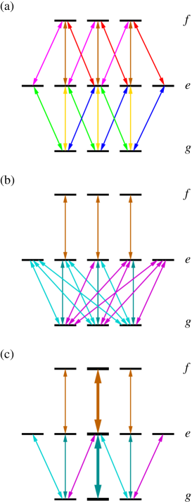
Figure 4: (Color Online) The three frames show the stages of the MS transformations when the sequence of degenerate states violates the condition Eq. (5): Frame (a) depicts the original coupling scheme , here $N_{f}<N_{e}$. Frame (b) shows the result of the Stokes field MS transformation, converting the couplings between $e$ and $f$ sets into independent one- and two-state systems. The one-state systems are in the $e$ set. Frame (c) shows the result of the pump field MS transformation followed by the redefinition of the sublevels in the $g$, $e$, and $f$ sets according to Eq. (65), leading to one dark state. This dark state is associated with the middle three-state linkage, indicated by heavy lines. In addition, the middle $e$ state is coupled not only to a single $g$ state but to the two others as well. As a result, the populations in the two spectator $g$ states may disturb the complete population transfer from the middle $g$ state, see text.

Therefore, we perform a second MS transformation, involving the $g$ set and just those states of the $e$ set that are decoupled from the $f$ set – two in the present example. The result is illustrated in Fig. (4c). In this example there is one $g$-set state that couples solely to an active MS state of the $e$ set because the other two have, by means of the MS transformation, been linked to the two uncoupled $e$ states. The population can be moved from this $g$ state to an $f$ state. The middle $e$ state is coupled to all three $g$ states. Consequently, if the two spectator $g$ states are populated, they disturb the complete population transfer from the middle $g$ state into $f$ states, and the population transfer process will place population into the $e$ and $f$ states.

In general, the transformation matrix of the second MS transformation is defined as

$${\bm{U}}^{\prime}=\left[\begin{array}[]{cccc}{\bm{A}}^{\prime}&{\bm{0}}&{\bm{0}}&{\bm{0}}\\ {\bm{0}}&{\bm{I}}&{\bm{0}}&{\bm{0}}\\ {\bm{0}}&{\bm{0}}&{\bm{B}}^{\prime}&{\bm{0}}\\ {\bm{0}}&{\bm{0}}&{\bm{0}}&{\bm{I}}\end{array}\right]\,.$$ (25)

The $N_{g}\times N_{g}$ unitary matrix ${\bm{A}}^{\prime}$ transforms the $g$ set, whereas the $(N_{e}-N_{f})\times(N_{e}-N_{f})$ unitary matrix ${\bm{B}}^{\prime}$ transforms the uncoupled states of the $e$ set. The two unit matrices ${\bm{I}}$ are of dimension $N_{f}\times N_{f}$. For $N_{e}-N_{f}<N_{g}$ the transformation yields

$${\bm{A}}^{\prime}\widetilde{\bm{P}}_{a} = \left[\begin{array}[]{c}\widetilde{\bm{P}}\\ \widetilde{\bm{P}}^{\prime}\end{array}\right]\,,$$ (26c)

$${\bm{A}}^{\prime}\widetilde{\bm{P}}_{b}{\bm{B}}^{\prime{\dagger}} = \left[\begin{array}[]{c}{\bm{0}}\\ \widetilde{\bm{\Pi}}\end{array}\right]\,,$$ (26f)

where the matrix $\widetilde{\bm{P}}$ is of dimension $[N_{g}-(N_{e}-N_{f})]\times N_{f}$, $\widetilde{\bm{P}}^{\prime}$ is of dimension $(N_{e}-N_{f})\times N_{f}$, and $\widetilde{\bm{\Pi}}$ is a diagonal matrix of dimension $(N_{e}-N_{f})\times(N_{e}-N_{f})$. For $N_{e}-N_{f}=N_{g}$ we find

$${\bm{A}}^{\prime}\widetilde{\bm{P}}_{a} = \widetilde{\bm{P}}^{\prime}\,,$$ (27a)

$${\bm{A}}^{\prime}\widetilde{\bm{P}}_{b}{\bm{B}}^{\prime{\dagger}} = \widetilde{\bm{\Pi}}\,,$$ (27b)

where the matrix $\widetilde{\bm{P}}^{\prime}$ is of dimension $N_{g}\times N_{f}$ and $\widetilde{\bm{\Pi}}$ is of dimension $N_{g}\times N_{g}$. We do not have $\widetilde{\bm{P}}$ in this case. Finally, for $N_{e}-N_{f}>N_{g}$ we get

$${\bm{A}}^{\prime}\widetilde{\bm{P}}_{a} = \widetilde{\bm{P}}^{\prime}\,,$$ (28a)

$${\bm{A}}^{\prime}\widetilde{\bm{P}}_{b}{\bm{B}}^{\prime{\dagger}} = \left[\begin{array}[]{cc}\widetilde{\bm{\Pi}}&{\bm{0}}\end{array}\right]\,,$$ (28c)

where the matrix $\widetilde{\bm{P}}^{\prime}$ is of dimension $N_{g}\times N_{f}$ and $\widetilde{\bm{\Pi}}$ is of dimension $N_{g}\times N_{g}$. Just as with the conditions $N_{e}-N_{f}=N_{g}$, we do not have a matrix $\widetilde{\bm{P}}$ in the present case either.

In general, none of the diagonal elements of the matrix $\widetilde{\bm{\Pi}}$ are zero. Therefore, when $N_{e}-N_{f}\geq N_{g}$ there are no states in the $g$ set that are coupled solely to active MS states in the $e$ set. It follows that no dark state can be identified in the system and hence a STIRAP-like population transfer is impossible.

In special (but important) cases it may occur that some diagonal elements of $\widetilde{\bm{\Pi}}$ vanish. Then the system has such MS $g$-set states that are coupled only to active MS states of the $e$ set, hence the system has dark states and a STIRAP process is possible. We will reconsider this case later in this subsection.

In all three cases $N_{e}-N_{f}>N_{g}$, $N_{e}-N_{f}=N_{g}$, and $N_{e}-N_{f}<N_{g}$ some initial population of the $g$ set cannot be included in the dark states of the system in the general case of arbitrary initial superposition of $g$ states. We conclude that in general in the case of $N_{g},N_{f}<N_{e}$ it is impossible to remove all the population from the $g$ set in a STIRAP-like population transfer process. Exceptions occur when the matrix $\widetilde{\bm{\Pi}}$ is identically zero. Then the uncoupled MS states of the $e$ set are decoupled not only from the $f$ set, but also from the $g$ set.

When $N_{e}-N_{f}<N_{g}$ the second MS transformation produces from the Hamiltonian of Eq. (24) the matrix

$${\widetilde{{\bm{H}}}}^{\prime}(t)=\left[\begin{array}[]{ccccc}{\bm{0}}&{\bm{0}}&p(t)\widetilde{{\bm{P}}}&{\bm{0}}&{\bm{0}}\\ {\bm{0}}&{\bm{0}}&p(t)\widetilde{{\bm{P}}}^{\prime}&p(t)\widetilde{{\bm{\Pi}}}&{\bm{0}}\\ p(t)\widetilde{{\bm{P}}}^{\dagger}&p(t)\widetilde{{\bm{P}}}^{\prime\dagger}&\hbar{\bm{\Delta}}&{\bm{0}}&s(t)\widetilde{\bm{\Sigma}}\\ {\bm{0}}&p(t)\widetilde{{\bm{\Pi}}}^{{\dagger}}&{\bm{0}}&\hbar{\bm{\Delta}}&{\bm{0}}\\ {\bm{0}}&{\bm{0}}&s(t)\widetilde{\bm{\Sigma}}^{\dagger}&{\bm{0}}&{\bm{0}}\\ \end{array}\right]\,.$$ (29)

The situation $N_{e}-N_{f}\geq N_{g}$ can be treated similarly. In order to find the dark states of the Hamiltonian of Eq. (29) we proceed in the same way as in Sec. IV.1. The eigenvectors are parameterized as

$$\widetilde{{\bm{\Phi}}}_{k}(t)=\left[\begin{array}[]{c}\widetilde{\bm{x}}_{k}(t)\\ \widetilde{\bm{x}}^{\prime}_{k}(t)\\ \widetilde{\bm{y}}_{k}(t)\\ \widetilde{\bm{y}}^{\prime}_{k}(t)\\ \widetilde{\bm{z}}_{k}(t)\\ \end{array}\right]\,.\quad\begin{array}[]{c}{g}\\ {g^{\prime}}\\ {e}\\ {e^{\prime}}\\ {f}\end{array}$$ (30)

The eigenvalue equation is defined by Eq. (11). By inserting the Hamiltonian of (29) and the parameterization of the eigenvector Eq. (30) into Eq. (11) we obtain five groups of coupled linear equations for $\widetilde{\bm{x}}_{k}$, $\widetilde{\bm{x}}^{\prime}_{k}$, $\widetilde{\bm{y}}_{k}$, $\widetilde{\bm{y}}^{\prime}_{k}$, and $\widetilde{\bm{z}}_{k}$. The $N_{D}$ linearly independent dark eigenvectors $\widetilde{{\bm{\Phi}}}_{0}^{(l)}(t)$ that belong to the eigenvalue $\varepsilon_{0}=0$, are given by

$$\widetilde{{\bm{\Phi}}}_{0}^{(l)}(t)={1\over{\cal N}_{0}(t)}\left[\begin{array}[]{c}s(t)\widetilde{\bm{x}}_{0}\\ s(t)\widetilde{\bm{x}}^{\prime}_{0}\\ {\bm{0}}\\ {\bm{0}}\\ -p(t)\widetilde{\bm{\Sigma}}^{-1}[\widetilde{{\bm{P}}}^{\dagger}\widetilde{\bm{x}}_{0}+\widetilde{{\bm{P}}}^{\prime\dagger}\widetilde{\bm{x}}^{\prime}_{0}]\end{array}\right]\,,$$ (31)

where, the constant vector $\widetilde{\bm{x}}^{\prime}_{0}$ should satisfy the extra condition

$$\widetilde{\bm{\Pi}}\widetilde{\bm{x}}^{\prime}_{0}={\bm{0}}\,.$$ (32)

This condition says that in a dark state no population can be in those $g$-set states that are linked to uncoupled $e$-set states. An example to this configuration is shown later in Sec. VI.3. The dimension $N_{D}$ of the dark subspace is equal to $N_{g}-(N_{e}-N_{f})$ plus the dimension of the zero-subspace of the matrix $\widetilde{\bm{\Pi}}$, Eq. (32), where we assumed that $N_{g}\geq(N_{e}-N_{f})$. For $N_{g}<(N_{e}-N_{f})$ the dimension of the dark subspace is equal to the dimension of the zero-subspace of the matrix $\widetilde{\bm{\Pi}}$.

It is useful to orthogonalize the dark states of Eq. (31). The orthogonality relation is given by Eq. (13). In this case we find that the vectors $[\widetilde{\bm{x}}^{(l)}_{0}\,\widetilde{\bm{x}}^{\prime(l)}_{0}]^{T}$, $l=1\ldots N_{D}$ should be the eigenvectors of the Hermitian matrix

$$\left[\begin{array}[]{c}\widetilde{\bm{P}}\\ \widetilde{\bm{P}}^{\prime}\end{array}\right]\widetilde{\bm{\Sigma}}^{-1\dagger}\widetilde{\bm{\Sigma}}^{-1}[\widetilde{{\bm{P}}}^{\dagger}\widetilde{{\bm{P}}}^{\prime\dagger}]\,,$$ (33)

with the restriction of Eq. (32).

The other eigenvectors, belonging to non-zero eigenvalues, are given by

$$\widetilde{{\bm{\Phi}}}_{k}(t)={1\over{\cal N}_{k}(t)}\left[\begin{array}[]{c}p(t)\widetilde{{\bm{P}}}\widetilde{\bm{y}}_{k}(t)\\ p(t)\left[\widetilde{{\bm{P}}}^{\prime}\widetilde{\bm{y}}_{k}(t)+\widetilde{{\bm{\Pi}}}\widetilde{\bm{y}}^{\prime}_{k}(t)\right]\\ \varepsilon_{k}(t)\widetilde{\bm{y}}_{k}(t)\\ \varepsilon_{k}(t)\widetilde{\bm{y}}^{\prime}_{k}(t)\\ s(t)\widetilde{\bm{\Sigma}}^{\dagger}\widetilde{\bm{y}}_{k}(t)\end{array}\right],$$ (34)

where ${\cal N}_{k}(t)$ is a normalization factor and the vector $[\widetilde{\bm{y}}_{k}(t)\,\widetilde{\bm{y}}^{\prime}_{k}(t)]^{T}$ satisfies the eigen-equation

$$\left[\begin{array}[]{cc}p(t)^{2}(\widetilde{{\bm{P}}}^{\dagger}\widetilde{{\bm{P}}}+\widetilde{{\bm{P}}}^{\prime\dagger}\widetilde{{\bm{P}}}^{\prime})+s(t)^{2}\widetilde{\bm{\Sigma}}\widetilde{\bm{\Sigma}}^{\dagger}&p(t)^{2}\widetilde{{\bm{P}}}^{\prime\dagger}\widetilde{{\bm{\Pi}}}\\ p(t)^{2}\widetilde{{\bm{\Pi}}}^{{\dagger}}\widetilde{{\bm{P}}}^{\prime}&p(t)^{2}\widetilde{{\bm{\Pi}}}^{{\dagger}}\widetilde{{\bm{\Pi}}}\end{array}\right]\left[\begin{array}[]{c}\widetilde{\bm{y}}_{k}(t)\\ \widetilde{\bm{y}}^{\prime}_{k}(t)\end{array}\right]=\varepsilon_{k}(t)[\varepsilon_{k}(t)-\hbar\Delta]\left[\begin{array}[]{c}\widetilde{\bm{y}}_{k}(t)\\ \widetilde{\bm{y}}^{\prime}_{k}(t)\end{array}\right]\,.$$ (35)

The states of Eq. (34) are bright states, because they include components from the $e$ set.

The eigenvectors of the Hamiltonian ${\bm{H}}(t)$ in the bare atomic basis can be obtained as

$${\bm{\Phi}}_{k}(t)={\bm{U}}^{\dagger}{\bm{U}}^{\prime\dagger}\left[\begin{array}[]{c}\widetilde{\bm{x}}_{k}(t)\\ \widetilde{\bm{x}}^{\prime}_{k}(t)\\ \widetilde{\bm{y}}_{k}(t)\\ \widetilde{\bm{y}}^{\prime}_{k}(t)\\ \widetilde{\bm{z}}_{k}(t)\\ \end{array}\right]=\left[\begin{array}[]{c}{\bm{A}}^{\prime\dagger}\left[\begin{array}[]{c}\widetilde{\bm{x}}_{k}(t)\\ \widetilde{\bm{x}}^{\prime}_{k}(t)\\ \end{array}\right]\\ \\ {\bm{B}}^{\dagger}\left[\begin{array}[]{c}\widetilde{\bm{y}}_{k}(t)\\ {\bm{B}}^{\prime\dagger}\widetilde{\bm{y}}^{\prime}_{k}(t)\\ \end{array}\right]\\ \\ {\bm{A}}^{\dagger}\widetilde{\bm{z}}_{k}(t)\end{array}\right]\,.$$ (36)

V Adiabaticity conditions and time evolution

In Sec. III we have presented the dark states of our degenerate system. Once we have the dark states we may consider adiabatic evolution of the system in the dark subspace. There are two questions that should be addressed in connection with adiabatic evolution:

• What are the conditions needed to ensure adiabatic evolution?

• If there are several degenerate dark states of a system, in general there are nonadiabatic couplings among them. How can we find the time evolution of the system in this case?

To answer the first question we apply the basic theory of adiabatic evolution Messiah , which assures that the evolution is adiabatic if any nonadiabatic couplings among the adiabatic states are negligible compared with their energy separation. In our model system we have a dark subspace that is spanned by states that have eigenvalue zero. The other adiabatic states, the bright states, have non-zero eigenvalues. Because we want the state vector to remain in the dark subspace, we require that the dark subspace be separated from the bright one, as expressed by the condition

$$\hbar|\langle\widetilde{\Phi}^{(l)}_{0}(t)|\dot{\widetilde{\Phi}}_{k}(t)\rangle|\ll|\varepsilon_{k}(t)|\,,$$ (37)

where $l=1\ldots N_{D}$ and $k=1\ldots N_{B}$, with $N_{B}$ being the number of bright states. The dot denotes time derivative. We may insert into Eq. (37) any set of dark and bright states from Sec. III. For example using the dark states given by Eq. (12) and the bright states from Eq. (17) we find

$$\frac{\hbar}{{\cal N}^{(l)}_{0}(t){\cal N}_{k}(t)}\left|s(t)\dot{p}(t)-p(t)\dot{s}(t)\right|\cdot\left|\langle{\bm{x}}^{(l)}_{0}|{\bm{P}}|{\bm{y}}_{k}(t)\rangle\right|\ll{|\varepsilon_{k}(t)|}\,.$$ (38)

This formula closely resembles the adiabaticity condition of the conventional nondegenerate three-level STIRAP AAMOP ,

$$\frac{1}{\Omega_{0}^{2}(t)}\left|S(t)\dot{P}(t)-P(t)\dot{S}(t)\right|\left|\begin{array}[]{c}\sin\varphi\\ \cos\varphi\end{array}\right|\ll\Omega_{0}(t)\left|\begin{array}[]{c}\cot\varphi\\ \tan\varphi\end{array}\right|\,,$$ (39)

with $\Omega_{0}(t)$ and $\varphi$ defined as

$$\Omega_{0}(t)=\sqrt{P^{2}(t)+S^{2}(t)}\,,\qquad\tan 2\varphi=\frac{\Omega_{0}(t)}{\Delta}\,,$$ (40)

respectively. The second factor on the lhs of Eq. (38) contains the time-derivatives of the envelope functions of the pump and Stokes pulses, whereas the third factor involves the element of the matrix ${\bm{P}}$ between the $l$th dark state at the initial time and the excited-state-amplitudes of the $k$th bright state at time $t$. On the rhs $\varepsilon_{k}$ is the eigenenergy associated with the $k$th bright state. Whenever the adiabaticity conditions Eq. (38) are fulfilled for all dark and bright states of the system, then the dark and bright subspaces evolve independently.

There remains the task of determining the time evolution in the dark subspace. When there are several degenerate dark states there are usually nonadiabatic couplings among them. In case of the tripod system Unanyan98 ; Theuer99 , due to the special choice for the time-dependence of the Stokes pulses, the two dark states mix throughout the population transfer process. If the dimension of the dark subspace is larger than two, then in general there is no exact analytic solution Kis01 ; Kis02 . In our case the situation is much simpler. The nonadiabatic coupling between a pair of dark states is $\langle\widetilde{\Phi}^{(l)}_{0}(t)|\dot{\widetilde{\Phi}}^{(k)}_{0}(t)\rangle\,$. By evaluating this expression for any pair of dark states from Sec. IV we always get identically zero. Hence the dark states do not mix throughout the whole transfer process. This property simplifies the calculations considerably, since the time evolution operator in the dark subspace is given by

$${\bm{U}}(t,t_{0})=\sum_{l=1}^{N_{D}}|{\Phi}^{(l)}_{0}(t)\rangle\langle{\Phi}^{(l)}_{0}(t_{0})|\,.$$ (41)

For example, for $N_{g}\leq N_{e}\leq N_{f}$ the vectors ${\bm{\Phi}}^{(l)}_{0}(t_{0})$ are equal to ${\bm{x}}_{0}^{(l)}$ from Eqs. (12) and (13). Once we define the density matrix ${\bm{\varrho}}(t_{0})$ of the system at time $t_{0}$ the density matrix at any later time is given by

$${\bm{\varrho}}(t)={\bm{U}}(t,t_{0}){\bm{\varrho}}(t_{0}){\bm{U}}^{{\dagger}}(t,t_{0})\,,$$ (42)

provided that the adiabaticity conditions Eq. (38) are satisfied. Note that this formula is valid only if ${\bm{\varrho}}(t_{0})$ lies entirely in the dark subspace. It follows from Eqs. (41) and (42) that any pure or mixed initial state of the system occupying the dark subspace of the $g$ set is transferred to the $f$ set in the course of the population transfer process. In the case of a pure initial state ${\Psi}(t_{0})$ we have

$${\Psi}(t)={\bm{U}}(t,t_{0}){\Psi}(t_{0})\,.$$ (43)

Here again, ${\Psi}(t_{0})$ must have components solely in the dark subspace. (Were the state vector to have components initially in the bright subspace, then adiabatic evolution would maintain such presence. Because the excited states undergo spontaneous emission, their populations have the potential to interrupt the coherence of the dynamics and thereby to diminish the population transfer.)

VI Some examples

In this section we demonstrate through some examples the usage of our method. To be specific, we consider atomic transitions where the origin of the degeneracy is the set of degenerate magnetic sublevels of angular momentum states in the absence of a magnetic field. Our purpose is to present some typical configurations that may occur in realistic situations.

VI.1 The $J=1\leftrightarrow 2\leftrightarrow 3$ linkage

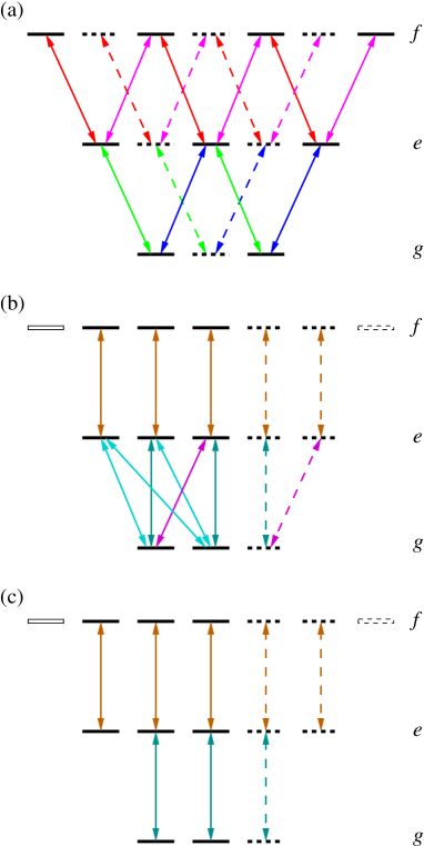
Figure 5: (Color Online) The coupling configuration

for the $J=1\leftrightarrow 2\leftrightarrow 3$ linkage with only $\sigma^{\pm}$ polarized coupling fields. The system separates into two independent subsystems; the smaller one is shown with dashed lines, the larger one with solid lines. Frame (b) shows the result of the Stokes-field MS transformation. Frame (c) shows the redefinition of the states in the $g$, $e$, and $f$ sets according to Eq. (65).

In this example we consider the linkage $J=1\leftrightarrow 2\leftrightarrow 3$, shown in Fig. 5 and assume that only $\sigma^{\pm}$ fields are present. In this case there are two independent coupled systems: the one with $M_{g}=0$, $M_{e}=\pm 1$, and $M_{f}=0,\pm 2$ (shown as dashed lines); and the other one with $M_{g}=\pm 1$, $M_{e}=0,\pm 2$, and $M_{f}=\pm 1,\pm 2$ (shown as full lines). The first one has been studied in ref. Kis03 , hence we do not consider it here. For the second, larger system, the pump coupling matrix $\bm{P}$ is given by

$$\bm{P}=\frac{\hbar}{2}\frac{\,\,1}{\sqrt{3}}\left[\begin{array}[]{ccc}\Omega_{P}^{(-)}&\frac{\,\,1}{\sqrt{6}}\Omega_{P}^{(+)}&0\vspace{5pt}\\ 0&\frac{\,\,1}{\sqrt{6}}\Omega_{P}^{(-)}&\Omega_{P}^{(+)}\end{array}\right]\,,$$ (44)

whereas the Stokes coupling matrix reads

$${\bm{S}}=\frac{\hbar}{2}\frac{\,\,1}{\sqrt{5}}\left[\begin{array}[]{cccc}\vspace{5pt}\Omega_{S}^{(-)}&\frac{\,\,1}{\sqrt{15}}\Omega_{S}^{(+)}&0&0\\ \vspace{5pt}0&\frac{\sqrt{2}}{\sqrt{5}}\Omega_{S}^{(-)}&\frac{\sqrt{2}}{\sqrt{5}}\Omega_{S}^{(+)}&0\\ 0&0&\frac{\,\,1}{\sqrt{15}}\Omega_{S}^{(-)}&\Omega_{S}^{(+)}\end{array}\right].$$ (45)

The numeric factors in front of the $\Omega$-s describe the Clebsch-Gordan coefficients. The Rabi frequencies are parameterized as

$$\Omega_{P}^{(+)} = \Omega_{P}\,e^{i\phi_{P}}\cos\eta\,,$$ (46a)

$$\Omega_{P}^{(-)} = \Omega_{P}\,e^{i\psi_{P}}\sin\eta\,,$$ (46b)

$$\Omega_{S}^{(+)} = \Omega_{S}\,e^{i\phi_{S}}\cos\theta\,,$$ (46c)

$$\Omega_{S}^{(-)} = \Omega_{S}\,e^{i\psi_{S}}\sin\theta\,,$$ (46d)

where the amplitudes $\Omega_{P,S}$ are nonnegative. The angles $\eta$ and $\theta$ characterize the pump and Stokes field polarizations, respectively.

Here $N_{g}<N_{e}<N_{f}$ ($2<3<4$), hence the derivation in Sec IV.1 can be applied. As a first step, we have to perform the Stokes field MS transformation. The eigenvalues $\lambda_{k}$ of the matrix ${\bm{S}}{\bm{S}}^{{\dagger}}$ are given by the roots of a cubic equation, see Eq. (74).

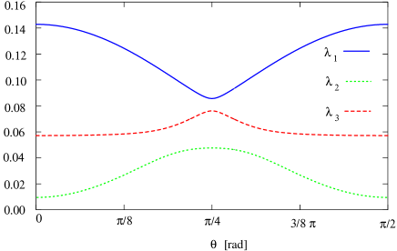
Figure 6: (Color Online) The eigenvalues of the matrix $\bm{S}\bm{S}^{{\dagger}}$, Eq. (45), as a function of the polarization of the Stokes field. The eigenvalues are measured in the units of $(\hbar\Omega_{S})^{2}$.

We display them in Fig. 6 as a function of the polarization angle $\theta$. They are never zero, hence the complete adiabatic population transfer is possible for any polarization of the Stokes field. However, their amplitudes depend on the polarization, which affects the adiabaticity conditions Eqs. (37) and (38). The Stokes field MS transformation matrices $\bm{A}$ and $\bm{B}$, Eq. (6), can be calculated in a straightforward manner; they are shown in the Appendix D. Since $N_{f}=N_{e}+1$, the Stokes field MS transformation yields a transformed coupling matrix $\widetilde{\bm{S}}$ in the form of the first row in Eq. (8). The diagonal part $\widetilde{\bm{\Sigma}}$ is given by

$$\widetilde{\bm{\Sigma}}=\frac{\sqrt{7}}{\sqrt{20}}\hbar\Omega_{S}\left[\begin{array}[]{ccc}\sqrt{\lambda_{1}}&0&0\\ 0&\sqrt{\lambda_{2}}&0\\ 0&0&\sqrt{\lambda_{3}}\end{array}\right]\,.$$ (47)

There are $2+4-3=3$ dark states in this system: one is in the $f$ set, an uncoupled state. The space of $g$ is two-dimensional, $N_{g}=2$, and hence there are two dark-states in the form of Eq. (12). The vectors ${\bm{x}}_{0}^{(k)}$ associated with these two dark states are the eigenvectors of the Hermitian matrix ${\bm{M}}$ of Eq. (14) and are given in the Appendix D. The two dark states are obtained by inserting their structure into Eq. (12) or, for the bare atomic basis, into Eq. (19).

We have performed numerical simulations to check the validity of our analytic results. In Fig. 7 initially the system was in the state $|g,J_{g}=1,M_{g}=1\rangle$. The envelope functions of the pump and Stokes pulses, respectively, are $p(t)=\exp(-[t-3]^{2}/6^{2})$ and $s(t)=\exp(-[t+3]^{2}/6^{2})$; and $\Omega_{P}=52$, $\Omega_{S}=42$. The polarizations are characterized by $\eta=1.3376$ rad, and $\theta=0.4636$ rad. The phases are chosen randomly as $\phi_{P}=1.1814$ rad, $\psi_{P}=0$ rad, $\phi_{S}=1.8925$ rad, and $\psi_{S}=2.8198$ rad. The detuning $\Delta$ is set to zero. We have found again very good agreement between the analytic calculations and the numeric simulation.

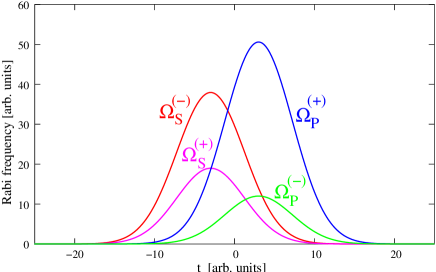
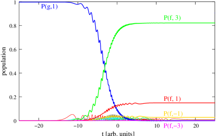
Figure 7: (Color Online) Upper frame: the pulse sequence used for the population transfer process in the coupled angular momentum system $J=1\leftrightarrow 2\leftrightarrow 3$. Initially only the state $|g,J_{g}=1,M_{g}=1\rangle$ was populated. Lower frame: The population evolution.

We also considered a mixed initial state, when the initial state of the system is chosen as half of the population is placed on each of the $|g,J_{g}=1,M_{g}=\pm 1\rangle$ states, and the coherence is zero between them. The numerically calculated dynamics is shown in Fig. 8. We can see that despite of the mixed initial state, the complete population can be transferred from the $g$ set to the $f$ set. The pulse sequence is the same as in the previous example.

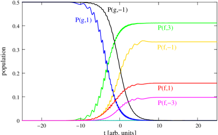
Figure 8: (Color Online) Same as Fig. 7, but for a mixed initial state, $P_{i}(1,-1)=P_{i}(1,1)=1/2$, all initial coherences are zero.

VI.2 The $J=1\leftrightarrow 1\leftrightarrow 1$ linkage

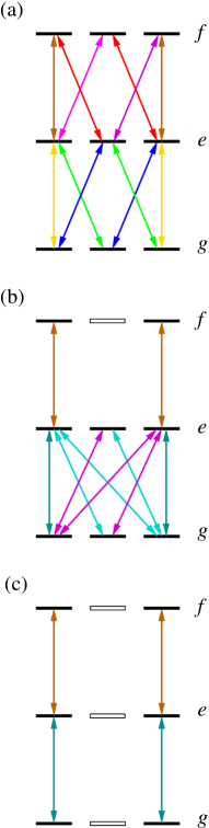
Figure 9: (Color Online) Same as Fig. 5 for equal state-degeneracies. For equal $J$-s, the $M=0\leftrightarrow 0$ transition is dipole-forbidden, and we cannot select a basis such that there occur couplings between all pairs of states of the degenerate sets. This restriction results from the property of the Clebsch-Gordan coefficients. Frame (c) shows the redefinition of the states in the $g$, $e$, and $f$ sets according to Eq. (65), leading to two independent three-state linkages.

As another example we consider the linkage $J=1\leftrightarrow 1\leftrightarrow 1$ shown in Fig. 9. In this case $N_{g}=N_{e}=N_{f}$, and hence the derivation in Sec. IV.1 is applicable. This is a counter-example to the general condition of Eq. (5): even though the condition Eq. (5) is satisfied, in this case the complete removal of an arbitrary population distribution from the $g$ set is impossible in the STIRAP way.

The coupling matrices $\bm{S}$ and $\bm{P}$ in the Hamiltonian Eq. (1) are given by

$$\bm{X}=\frac{\hbar}{2}\frac{1}{\sqrt{6}}\left[\begin{array}[]{ccc}\vspace{5pt}-\Omega_{X}^{(\pi)}&-\Omega_{X}^{(+)}&0\\ \vspace{5pt}[5pt]\Omega_{X}^{(-)}&0&-\Omega_{X}^{(+)}\\[5.0pt] 0&\Omega_{X}^{(-)}&\Omega_{X}^{(\pi)}\end{array}\right],$$ (48)

for $\bm{X}=\bm{S}$ or $\bm{P}$. The factor $1/\sqrt{6}$ and the $\pm$ signs describe the Clebsch-Gordan coefficients. The Rabi frequencies $\Omega_{X}^{(\pm,\pi)}$ correspond to the $\sigma^{+}$, $\sigma^{-}$, and $\pi$ polarizations, respectively. Note that a selection rule nullifies transitions $M=0\leftrightarrow M=0$.

As described in Sec. IV, we perform the Stokes-field MS transformation to diagonalize the Stokes coupling matrix ${\bm{S}}$. The eigenvalues of the matrix ${\bm{S}}{\bm{S}}^{{\dagger}}$ provide the squared moduli of the diagonal elements of the matrix $\widetilde{\bm{\Sigma}}=\widetilde{\bm{S}}={\bm{B}}{\bm{S}}{\bm{A}}^{{\dagger}}$, Eq. (7). They are given by

$$0,\quad\pm\frac{1}{6}\left(\Omega_{S}^{({\rm rms})}\right)^{2}\,,$$ (49)

with $\left(\Omega_{S}^{({\rm rms})}\right)^{2}=|\Omega_{S}^{(+)}|^{2}+|\Omega_{S}^{(-)}|^{2}+|\Omega_{S}^{(\pi)}|^{2}$. One of the eigenvalues is always zero and therefore, although the system satisfies the condition for complete population transfer, Eq. (5), the null Rabi frequency prevents complete transfer.

Fig. 10 demonstrates the population transfer in this system. Initially the system was in the state $(|g,J_{g}=1,M_{g}=-1\rangle-|g,J_{g}=1,M_{g}=0\rangle+|g,J_{g}=1,M_{g}=1\rangle)/\sqrt{3}$. The envelope functions of the pump and Stokes pulses, respectively, are chosen as $p(t)=\exp(-[t-2]^{2}/4^{2})$ and $s(t)=\exp(-[t+2]^{2}/4^{2})$, and $\Omega_{P}=\Omega_{S}=30$. The intensity is equally distributed among the $\sigma^{+}$, $\sigma^{-}$, and $\pi$ components of the exciting fields. The detuning $\Delta$ is set to zero. We have found excellent agreement between the analytic calculations and the numeric simulation. The adiabaticity conditions, Eq. (38), are also fulfilled throughout the relevant part of the population transfer process.

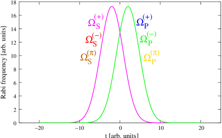
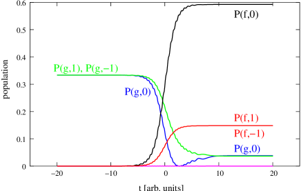
Figure 10: (Color Online) Upper frame: the pulse sequence used for the population transfer process in the coupled angular momentum system $J=1\leftrightarrow 1\leftrightarrow 1$. Initially the state $(|g,J_{g}=1,M_{g}=-1\rangle-|g,J_{g}=1,M_{g}=0\rangle+|g,J_{g}=1,M_{g}=1\rangle)/\sqrt{3}$ was populated. Lower frame: The population evolution. Part of the population is left in the $g$ set, because some of the MS Rabi frequencies vanish.

VI.3 The $J=1\leftrightarrow 2\leftrightarrow 1$ linkage

In our last example we consider the linkage $J=1\leftrightarrow 2\leftrightarrow 1$, shown in Fig. 11 and assume that only $\sigma^{\pm}$ fields are present. In this case there are two independent coupled systems: the one with $M_{g}=0$, $M_{e}=\pm 1$, and $M_{f}=0$ (shown as dashed lines) discussed recently in ref. Shah02 , and the other one with $M_{g}=\pm 1$, $M_{e}=0,\pm 2$, and $M_{f}=\pm 1$ (shown as full lines). This is a twin diamond configuration. For the larger system, the pump coupling matrix $\bm{P}$ is given by

$${\bm{P}}=\frac{\hbar}{2}\left[\begin{array}[]{ccc}\frac{\,\,1}{\sqrt{3}}\Omega_{P}^{(-)}&\frac{\,\,1}{\sqrt{18}}\Omega_{P}^{(+)}&0\\ \vspace{5pt}0&\frac{\,\,1}{\sqrt{18}}\Omega_{P}^{(-)}&\frac{\,\,1}{\sqrt{3}}\Omega_{P}^{(+)}\end{array}\right]\,.$$ (50)

whereas the Stokes coupling matrix reads

$${\bm{S}}=\frac{\hbar}{2}\left[\begin{array}[]{cc}\frac{\sqrt{3}}{5}\Omega_{S}^{(-)}&0\\ \vspace{5pt}\frac{\,\,1}{\sqrt{50}}\Omega_{S}^{(+)}&\frac{\,\,1}{\sqrt{50}}\Omega_{S}^{(+)}\\ \vspace{5pt}0&\frac{\sqrt{3}}{5}\Omega_{S}^{(-)}\end{array}\right]\,.$$ (51)

The parameterization of the Rabi frequencies $\Omega_{X}^{(\pm)}$ is given by Eq. (46). Here $N_{g},N_{f}<N_{e}$ ($2,2<3$), hence the derivation in Sec IV.3 is applicable. The sequence of the dimension of the subspaces violate the condition $N_{g}\leq N_{e}\leq N_{f}$, therefore, in general a STIRAP-like complete population transfer is not possible. However, this is another counter-example to the general condition of Eq. (5): even though the condition Eq. (5) is violated, we show that the complete removal of an arbitrary population distribution from the $g$ set is possible in the STIRAP way for a special choice of pulse polarizations and phases.

As usual, we start with the Stokes field MS transformation. The eigenvalues of the matrix ${\bm{S}}{\bm{S}}^{{\dagger}}$ are given by the roots of a quadratic equation, which read

$$\lambda_{1,2}=\frac{7}{100}\pm\frac{1}{100}\sqrt{24\cos^{2}2\theta+1}\,.$$ (52)

The Stokes field MS transformation matrices $\bm{A}$ and $\bm{B}$, Eq. (6), can be calculated in a straight forward manner, they are shown in the Appendix E. Since $N_{f}=N_{e}-1$, the Stokes field MS transformation yields a transformed coupling matrix $\widetilde{\bm{S}}$ in the form of the last row in Eq. (8). The diagonal part $\widetilde{\bm{\Sigma}}$ is given by

$$\widetilde{\bm{\Sigma}}=\frac{\hbar}{2}\Omega_{S}\left[\begin{array}[]{cc}\sqrt{\lambda_{1}}&0\\ 0&\sqrt{\lambda_{2}}\end{array}\right]\,.$$ (53)

The eigenvalues of Eq. (52) are always positive, hence this matrix is nonsingular for any polarization of the Stokes field. The Stokes field MS transformation yields two $e-f$ linkages and an $e$ state which is not coupled to any $f$ state, see Fig. 11b. Now, following the derivation of Sec IV.3 we perform a second MS transformation for the pump field. The transformation matrix is given by Eq. (25). In our case, the $2\times 2$ unitary matrix ${\bm{A}}^{\prime}$ is defined as

$${\bm{A}}^{\prime}=\left[\begin{array}[]{cc}\cos\theta&e^{-i(\psi_{S}-\phi_{S})}\sin\theta\\ e^{-\frac{1}{2}i(\phi_{S}-\psi_{S}+\phi_{P}+\psi_{P})}\sin\theta&-e^{-\frac{1}{2}i(\psi_{S}-\phi_{S}+\phi_{P}+\psi_{P})}\cos\theta\end{array}\right]\,,$$ (54)

while the matrix ${\bm{B}}^{\prime}$ is a scalar now, and chosen as unity. Since in this case $N_{e}-N_{f}<N_{g}$ ($3-2<2$), the transformed pump field coupling matrix takes the form of Eq. (26). The matrix $\widetilde{\bm{\Pi}}$ is a scalar, that reads

$$\widetilde{\bm{\Pi}}=\begin{array}[]{c}-\frac{\Omega_{P}}{2\sqrt{3}\sqrt{2-\cos^{2}2\theta}}\left(\cos\eta\cos\theta e^{\frac{1}{2}i(\psi_{S}-\phi_{S}+\phi_{P}-\psi_{P})}-\sin\eta\sin\theta e^{-\frac{1}{2}i(\psi_{S}-\phi_{S}+\phi_{P}-\psi_{P})}\right)\end{array}\,.$$ (55)

This is nonzero in general, hence one of the $g$ states is linked to the uncoupled $e$ state. Therefore, there is one dark state in the system, which reads

$$\widetilde{\bm{\Phi}}_{0}^{(1)}(t)=\frac{1}{{\cal N}_{0}^{(1)}(t)}\left[\begin{array}[]{c}s(t)\\ 0\\ 0\\ 0\\ 0\\ -p(t)\widetilde{\bm{\Sigma}}^{-1}\bm{B}_{a}\bm{P}^{\dagger}{\bm{A}^{\prime}}^{\dagger}\left[\begin{array}[]{c}1\\ 0\end{array}\right]\end{array}\right]\,.$$ (56)

This dark state is associated with the three-state linkage in the middle of Fig. 11c, indicated by heavy lines.

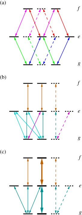
Figure 11: (Color Online) Same as Fig. 5 for the $J=1\leftrightarrow 2\leftrightarrow 1$ linkage with only $\sigma^{\pm}$ polarized coupling fields. The system separates into two independent subsystems; The smaller one is shown with dashed lines, the larger one with solid lines. Frame (b) shows the result of the Stokes-field MS transformation. Frame (c) shows the result of the pump field MS transformation and redefinition of the states in the $g$, $e$, and $f$ sets according to Eq. (65). In general, there is one dark state in the larger system which is associated with the three-state linkage indicated by heavy lines.

However, for

$$\psi_{S}-\phi_{S}+\phi_{P}-\psi_{P} = k\pi\,,$$ (57a)

$$\theta+(-1)^{k}\eta=\frac{1}{2}\pi\,,$$ (57b)

where $k$ is an integer, the scalar $\widetilde{\bm{\Pi}}$ vanishes. As a result, the uncoupled $e$ state becomes decoupled from the $g$ state as well. Therefore, beside the dark state of Eq. (56) there is an other one

$$\widetilde{\bm{\Phi}}_{0}^{(2)}(t)=\frac{1}{{\cal N}_{0}^{(2)}(t)}\left[\begin{array}[]{c}0\\ s(t)\\ 0\\ 0\\ 0\\ -p(t)\widetilde{\bm{\Sigma}}^{-1}\bm{B}_{a}\bm{P}^{\dagger}{\bm{A}^{\prime}}^{\dagger}\left[\begin{array}[]{c}0\\ 1\end{array}\right]\end{array}\right]\,.$$ (58)

In summary: complete population transfer is possible from the $g$ set to the $f$ set for the special choice of pulse polarizations and phases Eq. (57). It is important to note that the condition for complete transfer Eq. (57) is equivalent to that for the diamond configuration Shah02 . Hence, the population from the total $g$ set can be transferred into the $f$ set if the condition Eq. (57) is fulfilled.

Fig. 12 demonstrates the population transfer in the twin diamond configuration. Initially the system was in the state $\cos(\alpha)|g,J_{g}=1,M_{g}=-1\rangle+\sin(\alpha)|g,J_{g}=1,M_{g}=1\rangle$ with $\alpha=\arctan(1/3)$. The envelope functions of the pump and Stokes pulses are chosen as in Sec. VI.2. The polarization of the pump and Stokes pulses were chosen as $\eta=2\pi/5$ and $\theta=-\pi/7$, respectively. All phases of the pulses are zero. The detuning $\Delta$ is set to zero. After the pulse sequence has passed, some population is left in the $g$ and $e$ sets because the polarizations of the pulses violate the special condition for complete transfer Eq. (57). Finally, in Fig. 13 the polarizations of the pump and Stokes pulses are chosen so that the special condition Eq. (57) is fulfilled. Then, a complete population transfer occurs, all population from the $g$ set is moved into the $f$ set.

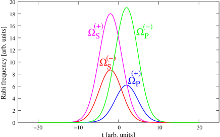
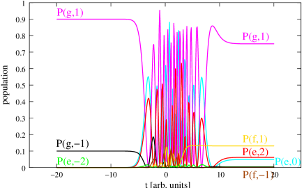
Figure 12: (Color Online) Upper frame: the pulse sequence used for the population transfer process in the coupled angular momentum system $J=1\leftrightarrow 2\leftrightarrow 1$. Initially the state $\cos(\alpha)|g,J_{g}=1,M_{g}=-1\rangle+\sin(\alpha)|g,J_{g}=1,M_{g}=1\rangle$ with $\alpha=\arctan(1/3)$ was populated. Lower frame: The population evolution. The pulses are chosen so that the special condition for complete transfer Eq. (57) is violated, hence part of the population is left in the $g$ and $e$ sets.

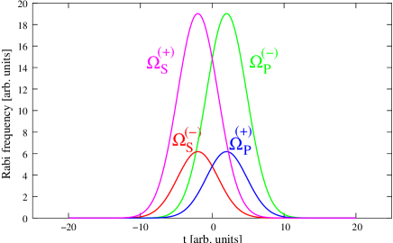
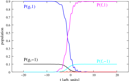
Figure 13: (Color Online) Same as Fig. 12, but now the special condition for the pulse polarizations Eq. (57) is fulfilled. Upper frame: the pulse sequence used for the population transfer process. The polarizations for the pump and Stokes pulses are $\eta=2\pi/5$ and $\theta=\pi/10$, respectively. Lower frame: The population evolution. All population is transferred from the $g$ set into the $f$ set.

VII Summary

We have considered the extension of the well-known STIRAP process in degenerate systems in which $N_{g}$ degenerate states of the $g$ set are coupled by means of a pump pulse to $N_{e}$ degenerate states of the $e$ set, which in turn are linked by the Stokes pulse to $N_{f}$ degenerate states of the $f$ set. We have shown that such a generalized STIRAP process is always possible if the succession of state-degeneracies is nondecreasing, i.e. $N_{g}\leq N_{e}\leq N_{f}$; and the number of non-vanishing MS Rabi frequencies is at least $N_{g}$ for both the pump and Stokes couplings. When such conditions hold, then for arbitrary couplings among states (e.g. arbitrary elliptical polarization of electric dipole radiation between magnetic sublevels) it is possible to obtain complete adiabatic passage of all population from the states of the $g$ set into some combination of states of the $f$ set. In this process the initial state is arbitrary, it can be any pure or mixed state that occupy the $g$ set.

An important exception from the above rule occurs in coupled angular momentum systems, when $J_{g}=J_{e}=J_{f}$. Then, due to the symmetry of the Clebsch-Gordan coefficients some couplings vanish, which results in incomplete transfer.

We have examined the possibility of adiabatic passage when this restriction on degeneracies does not hold. We have shown that part of the population can be transferred to the $f$ set. We have also pointed out that, for certain choices of the polarizations of the coupling fields, complete adiabatic population transfer can be obtained.

We have demonstrated that our scheme can be a powerful tool for coherent control of the quantum state in a degenerate system: in our proposal the selective addressing of individual states in the degenerate sets is not required. Nevertheless, the final state can be tailored by varying the polarizations and the relative phases of the coupling fields. We have shown through some specific examples that the control of the final superposition state is possible; the level of control depends on the system under consideration.

Appendix A Dipole Transition Moments

A common situation where degeneracy occurs is when the atomic states are eigenstates of angular momentum, bearing the labels $J$ and $M$. Then the dipole moments can be expressed in terms of Clebsch-Gordan coefficients and reduced matrix elements. For the pump transition ($g-e$) the general pattern of the dipole-transition matrix elements, for arbitrary polarization, is

$$\mu_{ij}=(g|\mu|e)\sum_{q}\epsilon_{q}^{(p)}\frac{(J_{g}M_{i},1q|J_{e}M_{j})}{\sqrt{2J_{g}+1}}\,,\quad\left\{\begin{array}[]{l}i=1\cdots N_{g}\\ j=1\cdots N_{e}\end{array}\right.\,,$$ (59)

where $(g|\mu|e)$ is the reduced matrix element and $\epsilon_{q}^{(p)}$ parameterizes the contribution of spherical component $q$ to the interaction. The Stokes transition moments are similarly written as

$$\mu_{ij}=(e|\mu|f)\sum_{q}\epsilon_{q}^{(S)}\frac{(J_{e}M_{i},1q|J_{f}M_{j})}{\sqrt{2J_{e}+1}}\,,\quad\left\{\begin{array}[]{l}i=1\cdots N_{e}\\ j=1\cdots N_{f}\end{array}\right..$$ (60)

For vibrational transitions in molecules the reduced matrix element must include a Franck-Condon factor.

Appendix B Singular coupling matrix $\widetilde{\bm{\Sigma}}$

Let us consider the Hamiltonian Eq. (1) in the MS basis, Eq. (7). The MS transformation of the coupling matrix ${\bm{S}}$ may result in three different forms, shown in Eq. (8). We obtain a diagonal matrix $\widetilde{\bm{\Sigma}}$ to which are appended either rows (if $N_{f}<N_{e}$) or columns (if $N_{f}>N_{e}$) of zero values. In the discussions of Sec. III we have assumed that the matrix $\widetilde{\bm{\Sigma}}$ is nonsingular. Here we consider the case when some diagonal elements of $\widetilde{\bm{\Sigma}}$ are zero. Let us choose the MS transformation matrices ${\bm{A}}$ and ${\bm{B}}$ in Eq. (6) in such a way that the zero diagonal elements appear in the bottom right corner of $\widetilde{\bm{\Sigma}}$. This non-zero part is denoted by $\widetilde{\bm{\Sigma}}_{C}$. Let the dimension of this matrix be $N_{C}\times N_{C}$. In this notation, instead of Eq. (8) we have

$$\widetilde{\bm{S}}=\left[\begin{array}[]{cc}\widetilde{\bm{\Sigma}}_{C}&{\bm{0}}\\ {\bm{0}}&{\bm{0}}\end{array}\right]\,,$$ (61)

where the number of all zero rows is $N_{e}-N_{C}$ and the number of all zero columns is $N_{f}-N_{C}$. From this form of the Stokes coupling matrix it is clearly seen that we have $N_{e}-N_{C}$ uncoupled MS states in the $e$ set and $N_{f}-N_{C}$ uncoupled MS states in the $f$ set. By inserting the coupling matrix Eq. (61) into the transformed Hamiltonian of Eq. (7) and performing a second MS transformation as in Sec. IV.3 among the $g$ set and the uncoupled MS states of the $e$ set we get

$$\widehat{\widetilde{{\bm{H}}}}(t)=\left[\begin{array}[]{cccccc}{\bm{0}}&{\bm{0}}&p(t)\widetilde{{\bm{P}}}&{\bm{0}}&{\bm{0}}&{\bm{0}}\\ {\bm{0}}&{\bm{0}}&p(t)\widetilde{{\bm{P}}}^{\prime}&p(t)\widetilde{{\bm{\Pi}}}&{\bm{0}}&{\bm{0}}\\ p(t)\widetilde{{\bm{P}}}^{\dagger}&p(t)\widetilde{{\bm{P}}}^{\prime\dagger}&\hbar{\bm{\Delta}}&{\bm{0}}&s(t)\widetilde{\bm{\Sigma}}_{C}&{\bm{0}}\\ {\bm{0}}&p(t)\widetilde{{\bm{\Pi}}}^{{\dagger}}&{\bm{0}}&\hbar{\bm{\Delta}}&{\bm{0}}&{\bm{0}}\\ {\bm{0}}&{\bm{0}}&s(t)\widetilde{\bm{\Sigma}}_{C}^{\dagger}&{\bm{0}}&{\bm{0}}&{\bm{0}}\\ {\bm{0}}&{\bm{0}}&{\bm{0}}&{\bm{0}}&{\bm{0}}&{\bm{0}}\end{array}\right]\,.$$ (62)

This Hamiltonian is almost identical with the one in Eq. (29). The difference is that here on the bottom of the matrix we have some rows of zero values as well as some columns of zero values to the far right. The adiabatic states of this Hamiltonian can be found as in Sec. IV.3. The eigenvectors are parameterized as

$$\widetilde{{\bm{\Phi}}}_{k}=\left[\begin{array}[]{c}\widetilde{\bm{x}}_{k}\\ \widetilde{\bm{x}}^{\prime}_{k}\\ \widetilde{\bm{y}}_{k}\\ \widetilde{\bm{y}}^{\prime}_{k}\\ \widetilde{\bm{z}}_{k}\\ \widetilde{\bm{z}}^{\prime}_{k}\\ \end{array}\right].$$ (63)

The eigenvalue equation yields the set of equations as in Sec. IV.3 plus one more equation for ${\bm{z}}^{\prime}_{k}$

$${\bm{0}}=\varepsilon_{k}{\bm{z}}^{\prime}_{k}\,.$$ (64)

When looking for the eigenstates belonging to the eigenvalue zero we set $\varepsilon_{0}=0$ in Eq. (64). Since ${\bm{z}}^{\prime}_{0}$ does not appear in the other equations, its value is determined from the initial condition of the system. Our usual assumption is that initially only the states of the $g$ set are occupied, therefore, ${\bm{z}}^{\prime}_{0}={\bm{0}}$. For the eigenstates with non-zero eigenvalues the only way to satisfy Eq. (64) is to set ${\bm{z}}^{\prime}_{k}$ to a null vector , ${\bm{z}}^{\prime}_{k}={\bm{0}}$. The eigenstates associated with non-zero eigenvalues $\varepsilon_{k}$ are given in Sec. IV.3.

Appendix C Linearization of the couplings $g\leftrightarrow e\leftrightarrow f$

The construction of the dark state Eq. (12) can be understood as follows. We introduce three sets of states, defined in the $g$, $e$, and $f$ sets, respectively

$$\mbox{$g$ set: }\widetilde{\widetilde{\psi}}_{g}^{(l)} = {\bm{x}}_{0}^{(l)}\,,\quad l=1\cdots N_{g}\,,$$ (65a)

$$\mbox{$e$ set: }\widetilde{\widetilde{\psi}}_{e}^{(l)} = \frac{1}{{\cal N}^{(l)}_{e}}\widetilde{{\bm{P}}}^{\dagger}{\bm{x}}_{0}^{(l)}\,,\quad l=1\cdots N_{g}\,,$$

$$+ N_{e}-N_{g}$$ other linearly independent states

$$\mbox{$f$ set: }\widetilde{\widetilde{\psi}}_{f}^{(l)} = \frac{1}{{\cal N}^{(l)}_{f}}\widetilde{\bm{\Sigma}}^{-1}\widetilde{{\bm{P}}}^{\dagger}{\bm{x}}_{0}^{(l)}\,,\quad l=1\cdots N_{g}\,,$$

$$+ \mbox{$N_{f}-N_{g}$ other linearly independent states}\,.$$

The vectors ${\bm{x}}_{0}^{(l)}$ are orthonormal by construction; ${\cal N}^{(l)}_{e}$ and ${\cal N}^{(l)}_{f}$ are appropriate normalization factors for the other components. The states in the $g$ and $f$ sets of Eq. (65) are orthonormal, but the states in the $e$ set of Eq. (65), though linearly independent and providing a complete set of excited states, are not orthogonal. The dual counterpart dual of the $e$ set of Eq. (65) reads

$$\mbox{dual $e$ set: }\widehat{\widehat{\psi}}_{e}^{(l)} = \frac{{\cal N}^{(l)}_{e}}{{\cal N}^{(l)\,2}_{f}}{\bm{x}}_{0}^{(l)\,T}\widetilde{\bm{P}}\widetilde{\bm{\Sigma}}^{-1{\dagger}}\widetilde{\bm{\Sigma}}^{-1}\,,$$

$$l=1\cdots N_{g}\,,$$

$$+ N_{e}-N_{g}$$ other linearly

independent states.

The vectors of these two sets are mutually orthogonal

$$\langle\widehat{\widehat{\psi}}_{e}^{(l)}|\widetilde{\widetilde{\psi}}_{e}^{(k)}\rangle=\delta_{kl}\,.$$ (67)

In the basis defined by Eqs. (65) the Hamiltonian of Eq. (9) reads

$$\widetilde{\widetilde{{\bm{H}}}}(t)=\left[\begin{array}[]{cccc}{\bm{0}}&p(t)\widetilde{{\bm{Q}}}_{1}&{\bm{0}}&{\bm{0}}\\ p(t)\widetilde{{\bm{Q}}}_{2}&\hbar{\bm{\Delta}}&s(t)\widetilde{\bm{\Sigma}}_{1}&{\bm{0}}\\ {\bm{0}}&s(t)\widetilde{\bm{\Sigma}}_{2}&{\bm{0}}&{\bm{0}}\\ {\bm{0}}&{\bm{0}}&{\bm{0}}&{\bm{0}}\end{array}\right]\,,$$ (68)

where $\widetilde{{\bm{Q}}}_{2}$ and $\widetilde{{\bm{\Sigma}}}_{1}$ are diagonal matrices with elements

$$(\widetilde{{\bm{Q}}}_{2})_{ll} = \frac{{\cal N}_{f}^{(l)2}}{{\cal N}_{e}^{(l)}}\,,\quad l=1\cdots N_{g}\,,$$

and

$$(\widetilde{{\bm{\Sigma}}}_{1})_{ll} = \frac{1}{{\cal N}_{f}^{(l)}}(\widetilde{{\bm{Q}}}_{2})_{ll}\,,\quad l=1\cdots N_{g}\,,$$ (69b)

respectively. It can be verified that the matrix elements of $\widetilde{\bm{P}}^{{\dagger}}$ is zero between the rest of the dual $e$ states and the $g$ states

$$\langle\widehat{\widehat{\psi}}_{e}^{(k)}|\widetilde{\bm{P}}^{{\dagger}}|\widetilde{\widetilde{\psi}}_{g}^{(l)}\rangle=0\,,\quad k=N_{g}+1\cdots N_{e}\,,\,\,l=1\cdots N_{g}\,.$$ (70)

Similarly, the matrix elements of $\widetilde{\bm{\Sigma}}$ is zero between the rest of the dual $e$ states and the first $N_{g}$ $f$ states

$$\langle\widehat{\widehat{\psi}}_{e}^{(k)}|\widetilde{\bm{\Sigma}}|\widetilde{\widetilde{\psi}}_{f}^{(l)}\rangle=0\,,\quad k=N_{g}+1\cdots N_{e}\,,\,\,l=1\cdots N_{g}\,.$$ (71)

The matrix elements of the other two symmetric, non-diagonal matrices $\widetilde{{\bm{Q}}}_{1}$ and $\widetilde{{\bm{\Sigma}}}_{2}$ are given by

$$(\widetilde{{\bm{Q}}}_{1})_{lk} = \frac{1}{{\cal N}_{e}^{(k)}}\langle{\bm{x}}_{0}^{(l)\,T}|\widetilde{\bm{P}}\widetilde{\bm{P}}^{{\dagger}}|{\bm{x}}_{0}^{(k)}\rangle\,,$$

and

$$(\widetilde{{\bm{\Sigma}}}_{2})_{lk} = \frac{1}{{\cal N}_{f}^{(l)}}(\widetilde{{\bm{Q}}}_{1})_{lk}\,.$$ (72b)

The dark states of the Hamiltonian (68) can be obtained in the same manner as in the above derivation that led to the dark states Eq. (12). The population transfer is described by the equation

$$p(t){\cal N}_{f}^{(l)}\widetilde{x}_{0}^{(l)}+s(t)\widetilde{\widetilde{z}}_{0}^{(l)}=0\,,$$ (73)

where the components $\widetilde{x}_{0}^{(l)}$ and $\widetilde{\widetilde{z}}_{0}^{(l)}$ are the probability amplitudes associated with the basis vectors Eqs. (65a) and (65) in the $g$ and $f$ sets, respectively. Hence in this basis the couplings $g\leftrightarrow e\leftrightarrow f$ provide independent pathways of excitation. Each $g$ state is connected through a single pathway to a single $f$ state.

Appendix D Stokes field MS transformation matrices for the $J=1\leftrightarrow 2\leftrightarrow 3$ linkage

The Stokes field MS transformation yields three eigenvalues $\lambda_{k}$ of the matrix ${\bm{S}}{\bm{S}}^{{\dagger}}$ composed from the Stokes field coupling matrix of Eq. (45)

$$\lambda_{k}=z+w\cot\left(\frac{1-k}{3}\pi+\frac{1}{3}\arctan v\right),$$ (74)

for $k=1,2,3$, where

$$u = \frac{3}{4}\sqrt{146004\cos 12\theta+857454\cos 8\theta+2234532\cos 4\theta+1524810}$$ (75a)

$$v = \frac{2u}{(839+909\cos 4\theta)}$$ (75b)

$$w = \frac{73002\cos 12\theta+428727\cos 8\theta+1117266\cos 4\theta+762405}{22960u+19320u\cos 4\theta}$$ (75c)

$$z = \frac{709\cos 4\theta+923}{14490\cos 4\theta+17220}.$$ (75d)

The Stokes field MS transformation matrix $\bm{A}$ is given by

$$\bm{A}=e^{i\phi_{S}}\left[\begin{array}[]{cccc}p_{1}^{(A)}(\lambda_{1})/n^{(A)}(\lambda_{1})&p_{2}^{(A)}(\lambda_{1})/n^{(A)}(\lambda_{1})&p_{3}^{(A)}(\lambda_{1})/n^{(A)}(\lambda_{1})&p_{4}^{(A)}(\lambda_{1})/n^{(A)}(\lambda_{1})\\ p_{1}^{(A)}(\lambda_{2})/n^{(A)}(\lambda_{2})&p_{2}^{(A)}(\lambda_{2})/n^{(A)}(\lambda_{2})&p_{3}^{(A)}(\lambda_{2})/n^{(A)}(\lambda_{2})&p_{4}^{(A)}(\lambda_{2})/n^{(A)}(\lambda_{2})\\ p_{1}^{(A)}(\lambda_{3})/n^{(A)}(\lambda_{3})&p_{2}^{(A)}(\lambda_{3})/n^{(A)}(\lambda_{3})&p_{3}^{(A)}(\lambda_{3})/n^{(A)}(\lambda_{3})&p_{4}^{(A)}(\lambda_{3})/n^{(A)}(\lambda_{3})\\ d_{1}^{(A)}/n_{d}^{(A)}&d_{2}^{(A)}/n_{d}^{(A)}&d_{3}^{(A)}/n_{d}^{(A)}&d_{4}^{(A)}/n_{d}^{(A)}\end{array}\right],$$ (76)

where the polynomials $p_{i}^{(A)}(x)$ and the normalization $n_{d}^{(A)}(x)$ read

$$p_{1}^{(A)}(x) = \frac{1}{8}e^{i(2\psi_{S}-2\phi_{S})}\sin\theta(14700x^{2}-980(2+\cos 2\theta)x+\cos 4\theta+56\cos 2\theta+63)\,,$$ (77a)

$$p_{2}^{(A)}(x) = \frac{\sqrt{15}}{24}e^{i(\psi_{S}-\phi_{S})}\cos\theta(2940x^{2}-(308+280\cos 2\theta)x+3\cos 4\theta+12\cos 2\theta+9)\,,$$ (77b)

$$p_{3}^{(A)}(x) = \frac{\sqrt{15}}{8}\sin\theta(28(1+\cos 2\theta)x-\cos 4\theta-4\cos 2\theta-3)\,,$$ (77c)

$$p_{4}^{(A)}(x) = \frac{1}{8}e^{i(\phi_{S}-\psi_{S})}\cos\theta(1-\cos 4\theta)\,,$$ (77d)

$$n^{(A)}(x) = \sqrt{\left|p_{1}^{(A)}(x)\right|^{2}+\left|p_{2}^{(A)}(x)\right|^{2}+\left|p_{3}^{(A)}(x)\right|^{2}+\left|p_{4}^{(A)}(x)\right|^{2}}\,,$$ (77e)

and the coefficients $$d_{i}^{(A)} n_{d}^{(A)}$$, and the normalization are defined as

$$d_{1}^{(A)} = -e^{i(2\psi_{S}-2\phi_{S})}\cot^{3}\theta\,,$$ (77f)

$$d_{2}^{(A)} = \sqrt{15}e^{i(\psi_{S}-\phi_{S})}\cot^{2}\theta\,,$$ (77g)

$$d_{3}^{(A)} = -\sqrt{15}\cot\theta\,,$$ (77h)

$$d_{4}^{(A)} = e^{i(\phi_{S}-\psi_{S})}\,,$$ (77i)

$$n_{d}^{(A)} = \sqrt{1+15\cot^{2}\theta+15\cot^{4}\theta+\cot^{6}\theta}\,.$$ (77j)

Similarly, the other Stokes field MS transformation matrix is obtained as

$$\bm{B}=\left[\begin{array}[]{ccc}p_{1}^{(B)}(\lambda_{1})/n^{(B)}(\lambda_{1})&p_{2}^{(B)}(\lambda_{1})/n^{(B)}(\lambda_{1})&p_{3}^{(B)}(\lambda_{1})/n^{(B)}(\lambda_{1})\\ p_{1}^{(B)}(\lambda_{2})/n^{(B)}(\lambda_{2})&p_{2}^{(B)}(\lambda_{2})/n^{(B)}(\lambda_{2})&p_{3}^{(B)}(\lambda_{2})/n^{(B)}(\lambda_{2})\\ p_{1}^{(B)}(\lambda_{3})/n^{(B)}(\lambda_{3})&p_{2}^{(B)}(\lambda_{3})/n^{(B)}(\lambda_{3})&p_{3}^{(B)}(\lambda_{3})/n^{(B)}(\lambda_{3})\end{array}\right],$$ (78)

where the polynomials $p_{i}^{(B)}(x)$ and the normalization $n_{d}^{(B)}(x)$ read

$$p_{1}^{(B)}(x) = e^{i(\phi_{S}-\psi_{S})}p_{1}^{(A)}(x)/\sin\theta\,,$$ (79a)

$$p_{2}^{(B)}(x) = \frac{\sqrt{6}}{12}\sin 2\theta(105x-7\cos 2\theta-8)\,,$$ (79b)

$$p_{3}^{(B)}(x) = \frac{1}{4}e^{i(\phi_{S}-\psi_{S})}\sin^{2}2\theta\,,$$ (79c)

$$n^{(B)}(x) = \sqrt{\left|p_{1}^{(B)}(x)\right|^{2}+\left|p_{2}^{(B)}(x)\right|^{2}+\left|p_{3}^{(B)}(x)\right|^{2}}\,.$$ (79d)

The vectors ${\bm{x}}_{0}^{(1,2)}$ characterizing the dark states of Eq. (12) are obtained by finding the eigenvectors of the Hermitian matrix Eq. (14), which is obtained by inserting Eqs. (44), (47) and (78) into Eq. (14). The two eigenvectors are given by

$${\bm{x}}_{0}^{(1)} = \left[\begin{array}[]{c}\sin\chi e^{i\xi}\\ \cos\chi\end{array}\right],$$ (80c)

$${\bm{x}}_{0}^{(2)} = \left[\begin{array}[]{c}\cos\chi e^{i\xi}\\ -\sin\chi\end{array}\right],$$ (80f)

where

$$\chi = \frac{1}{2}\arctan\frac{2|u^{\prime}|}{v^{\prime}},$$ (81a)

$$\xi = \arg u^{\prime},$$ (81b)

$$u^{\prime} = \frac{7}{60}e^{i(\phi_{S}-\psi_{S})}\sin 2\theta(-8+7\cos 2\theta\cos 2\eta)$$ (81c)

$$\quad+e^{i(\phi_{P}-\psi_{P})}\sin 2\eta\left[\frac{7}{24}+\left(\frac{343}{360}+\frac{7}{40}e^{2i(\phi_{S}-\psi_{S}+\psi_{P}-\phi_{P})}\right)\sin^{2}2\theta\right],$$

$$v^{\prime} = \frac{49}{60}\cos(\phi_{S}-\psi_{S}+\psi_{P}-\phi_{P})\sin 2\eta\sin 4\theta+\left(\frac{301}{36}+\frac{203}{90}\cos^{2}2\theta\right)\cos 2\eta-\frac{49}{5}\cos 2\theta.$$ (81d)

Appendix E Stokes field MS transformation matrices for the $J=1\leftrightarrow 2\leftrightarrow 1$ linkage

The Stokes field MS transformation matrix $\bm{A}$ is given by

$$\bm{A}=e^{i\psi_{S}}\left[\begin{array}[]{cc}p_{1}^{(A)}(\lambda_{1})/n^{(A)}(\lambda_{1})&p_{2}^{(A)}(\lambda_{1})/n^{(A)}(\lambda_{1})\\ p_{1}^{(A)}(\lambda_{2})/n^{(A)}(\lambda_{2})&p_{2}^{(A)}(\lambda_{2})/n^{(A)}(\lambda_{2})\end{array}\right]\,,$$ (82)

where the polynomials $p_{i}^{(A)}(x)$ and the normalization $n^{(A)}(x)$ read

$$p_{1}^{(A)}(x) = -1-5\sin^{2}\theta+50x,$$ (83)

$$p_{2}^{(A)}(x) = \sin\theta\cos\theta e^{-i(\psi_{S}-\phi_{S})},$$ (84)

$$n^{(A)}(x) = \sqrt{\left|p_{1}^{(A)}(x)\right|^{2}+\left|p_{2}^{(A)}(x)\right|^{2}}.$$ (85)

Similarly, the other Stokes field MS transformation matrix is obtained as

$$\bm{B}=\left[\begin{array}[]{c}\bm{B}_{a}\\ \bm{B}_{b}\end{array}\right]\,,$$ (86)

where

$$\bm{B}_{a}=\left[\begin{array}[]{cc}\mathrm{sgn}(\sin 4\theta\sin\theta)&0\\ 0&\mathrm{sgn}(\cos\theta)\end{array}\right]\left[\begin{array}[]{ccc}p_{1}^{(B)}(\lambda_{1})/n^{(B)}(\lambda_{1})&p_{2}^{(B)}(\lambda_{1})/n^{(B)}(\lambda_{1})&p_{3}^{(B)}(\lambda_{1})/n^{(B)}(\lambda_{1})\\ p_{1}^{(B)}(\lambda_{2})/n^{(B)}(\lambda_{2})&p_{2}^{(B)}(\lambda_{2})/n^{(B)}(\lambda_{2})&p_{3}^{(B)}(\lambda_{2})/n^{(B)}(\lambda_{2})\end{array}\right]\,,$$ (87)

and

$$\bm{B}_{b}=\left[\begin{array}[]{ccc}d_{1}^{(B)}/n_{d}^{(B)}&d_{2}^{(B)}/n_{d}^{(B)}&d_{3}^{(B)}/n_{d}^{(B)}\end{array}\right]\,.$$ (88)

The polynomials $p_{i}^{(B)}(x)$ with the normalization $n_{d}^{(B)}(x)$; the coefficients $d_{i}^{(B)}$ with the normalization $n_{d}^{(B)}$ read

$$p_{1}^{(B)}(x) = -e^{-i(\phi_{S}-\psi_{S})}\cos^{2}\theta(7\sin^{2}\theta+\cos^{2}\theta-50x)\,,$$ (89)

$$p_{2}^{(B)}(x) = \frac{\sqrt{6}}{4}\sin 4\theta\,,$$ (90)

$$p_{3}^{(B)}(x) = e^{-i(\psi_{S}-\phi_{S})}\sin^{2}\theta(7\cos^{2}\theta+sin^{2}\theta-50x)\,,$$ (91)

$$n^{(B)}(x) = \sqrt{\left|p_{1}^{(A)}(x)\right|^{2}+\left|p_{2}^{(A)}(x)\right|^{2}+\left|p_{3}^{(A)}(x)\right|^{2}}\,,$$ (92)

$$d_{1}^{(B)} = e^{i(\phi_{S}-\psi_{S})}\sin^{2}\theta\,,$$ (93)

$$d_{2}^{(B)} = -\sqrt{6}\sin\theta\cos\theta\,,$$ (94)

$$d_{3}^{(B)} = e^{i(\psi_{S}-\phi_{S})}\cos^{2}\theta\,,$$ (95)

$$n_{d}^{(B)} = \sqrt{1+\sin^{2}2\theta}\,.$$ (96)

References

- (1) N.V. Vitanov, M. Fleischhauer, B.W. Shore, and K. Bergmann, Adv. Atomic Mol. Opt. Phys. 46, 55 (2001).
- (2) J. Oreg, F. T. Hioe, J.H. Eberly, Phys. Rev. A 29, 690 (1984); J. R. Kuklinski, U. Gaubatz, F. T. Hioe, and K. Bergmann, Phys. Rev. A 40, 6741 (1989); U. Gaubatz, P. Rudecki, S. Schiemann, and K. Bergmann, J. Chem. Phys. 92, 5363 (1990).
- (3) N.V. Vitanov, T. Halfmann, B.W. Shore, and K. Bergmann, Ann. Rev. Phys. Chem. 52, 763 (2001)
- (4) B.W. Shore, K. Bergmann, J. Oreg, and S. Resenwaks, Phys. Rev. A 44, 7442 (1991).
- (5) A.V. Smith, J. Opt. Soc. Am. B 9, 1543 (1992).
- (6) P. Pillet, C. Valentin, R.-L. Yuan, and J. Yu, Phys. Rev. A 48, 845 (1993).
- (7) D.S. Weiss, B.C. Young, S. Chu, Appl. Phys. B 59, 217 (1994).
- (8) B.W. Shore, J. Martin, M.P. Fewell, K. Bergmann, Phys. Rev. A 52, 566 (1995).
- (9) J. Martin, B. W. Shore, and K. Bergmann, Phys. Rev. A 52, 583 (1995).
- (10) V.S. Malinovsky, D.J. Tannor, Phys. Rev. A 56, 4929 (1997).
- (11) N.V. Vitanov, Phys. Rev. A 58, 2295 (1998).
- (12) H. Theuer and K. Bergmann, Eur. Phys. J. D 2, 279 (1998).
- (13) P. Marte, P. Zoller and J.L. Hall, Phys. Rev. A 44, R4118 (1991).
- (14) J. Lawall and M. Prentiss, Phys. Rev. Lett. 72, 993 (1994).
- (15) L.S. Goldner, C. Gerz, R.J.C. Spreeuw, S.L. Rolston, C.I. Westbrook, W.D. Phillips, P. Marte, and P. Zoller, Phys. Rev. Lett. 72, 997 (1994).
- (16) M. Weitz, B.C. Young, and S. Chu, Phys. Rev. Lett. 73 2563 (1994).
- (17) R.G. Unanyan, M. Fleischhauer, B.W. Shore, and K. Bergmann, Opt. Commun. 155, 144 (1998).
- (18) H. Theuer, R.G. Unanyan, C. Habscheid, K. Klein, and K. Bergmann, Opt. Express 4, 77 (1999).
- (19) R.G. Unanyan, B.W. Shore, and K. Bergmann, Phys. Rev. A 59, 2910 (1999).
- (20) R.G. Unanyan, B.W. Shore, and K. Bergmann, Phys. Rev. A 63, 043401 (2001).
- (21) Z. Kis and S. Stenholm, Phys. Rev. A 64, 063406 (2001).
- (22) Z. Kis and S. Stenholm, J. Mod. Optics 49, 111 (2002).
- (23) P. Král, Z. Amitay, M. Shapiro, Phys. Rev. Lett. 89, 63002 (2002).
- (24) P. Král, M. Shapiro, Phys. Rev. A 65, 43413 (2002).
- (25) A. Karpati and Z. Kis, J. Phys. B 36, 905 (2003).
- (26) J. R. Morris and B. W. Shore, Phys. Rev. A 27, 906 (1983).
- (27) N.V. Vitanov, Z. Kis, and B. W. Shore, Phys. Rev. A 68, 063414 (2003).
- (28) S. Lipschutz, M.L. Lipson, Schaum’s Outline of Linear Algebra (McGraw-Hill).
- (29) A. Messiah, 1959, Mécanique Quantique (Paris: Dunod) pp.637-650.
- (30) S.P. Shah, D.J. Tannor, and S.A. Rice, Phys. Rev. A 66, 033405 (2002).