A Bohmian approach to quantum fractals

Abstract

A quantum fractal is a wavefunction with a real and an imaginary part continuous everywhere, but differentiable nowhere. This lack of differentiability has been used as an argument to deny the general validity of Bohmian mechanics (and other trajectory–based approaches) in providing a complete interpretation of quantum mechanics. Here, this assertion is overcome by means of a formal extension of Bohmian mechanics based on a limiting approach. Within this novel formulation, the particle dynamics is always satisfactorily described by a well defined equation of motion. In particular, in the case of guidance under quantum fractals, the corresponding trajectories will also be fractal.

1 Introduction

Quantum mechanics is the most powerful theory developed up to now to describe the physical world. However, its standard formulation, based on statistical grounds, does not provide an intuitive insight of microscopic phenomena as classical mechanics does for macroscopic ones. For example, the evolution of a system cannot be followed in the configuration space by means of well defined, individual trajectories. On the contrary, the wavefunction associated to such a system extends to the whole available space, describing the probability for the system to be located at each (space) point at a certain time.

In order to obtain a more intuitive picture of quantum phenomena, alternative approaches relying on the concept of trajectory have been proposed [1]. One of them is Bohmian mechanics [2, 3, 4]. This theory is not merely a reinterpretation of the standard quantum mechanics despite its equivalence at a predictive level, but a generalization of classical mechanics that accounts for quantum phenomena. Hence, since Bohmian mechanics formally rests on the same conceptual grounds as classical mechanics, the notion of trajectory (causally describing the particle evolution) can also be applied in a natural way to study of microscopic world without contradicting the statistical postulates of the standard quantum mechanics.

Recently, it has been argued [5] that trajectory–based theories, like Bohmian mechanics, fail in providing a complete interpretation of quantum mechanics. In particular, these theories could not satisfactorily deal with wavefunctions displaying fractal features, the so–called quantum fractals [6, 7, 8]. The existence of this class of wavefunctions in quantum mechanics has important consequences from a fundamental viewpoint: despite the coarse–graining restrictions implied by Heisenberg’s uncertainty principle, these wavefunctions constitute the proof that fractal objects can appear in quantum mechanics as well as in classical mechanics. Indeed, Wócik et al. [8] pointed out that quantum fractals could be experimentally constructed by considering heavy atoms or ions in macroscopic traps, where the number of energy levels would be large enough to observe scaling properties at least up to several orders of magnitude (what is considered a physical fractal). On the other hand, Amanatidis et al. [9] have observed theoretically this fractal behaviour during the ballistic and diffusive evolution of wave packets moving in tight–binding lattices, a study of interest in quantum information theory and quantum computation.

Here it is shown that the incompatibility between Bohmian mechanics and the existence of quantum fractals can be easily avoided by reformulating the particle equation of motion. This reformulation is based on a limiting approach, where the wavefunction is expanded in a series of eigenvectors of the Hamiltonian. If the wavefunction is not fractal, but regular, the trajectories are the same as directly computed by means of standard Bohmian mechanics. However, if the wavefunction presents fractal features, its non–differentiability forbids a direct calculation of the trajectories, which can be obtained, on the other hand, by means of the limiting approach proposed here. Thus, this formal extension of Bohmian mechanics, based on a novel reformulation of the particle equation of motion, provides a causal picture for any arbitrary wavefunction, regular or fractal.

The organization of this paper is as follows. In order to make the paper self–contained, a survey on quantum fractals is given in section 2. The fundamentals of Bohmian mechanics and its generalization to deal with quantum fractals are presented in section 3. The application of the new concepts introduced in this work is illustrated in detail in section 4 by means of the problem of a non–relativistic, spin–less particle of mass $m$ in a one–dimensional box. This simple, integrable problem can be considered a paradigm of fractals appearing under conditions not necessarily related to a chaotic dynamics [8]. In section 5 the question of the unbounded energy for quantum fractals and its interpretation in terms of quantum trajectories is discussed. Finally, the main conclusions derived from this work are summarized in section 6.

2 Quantum fractals

A general method [8] to construct quantum fractals with an arbitrary fractal dimension consists in using the quantum analog of the Weierstrass function [10]

$$W(x)=\sum_{r=0}^{\infty}b^{r}\sin(a^{r}x),\qquad a>1>b>0,\qquad ab\geq 1$$ (1)

the paradigm of continuous fractal function. Thus, for example, in the problem of a particle in a one–dimensional box of length $L$ (with $0<x<L$), solutions of the Schrödinger equation can be constructed as

$$\Phi_{t}(x;R)=A_{R}\sum_{r=0}^{R}n^{r(s-2)}\sin(p_{n,r}x/\hbar){\rm e}^{-{\rm i}E_{n,r}t/\hbar}$$ (2)

with $2>s>0$ and $n\geq 2$. Here, $p_{n,r}=n^{r}\pi\hbar/L$ and $E_{n,r}=p_{n,r}^{2}/2m$ are, respectively, the quantized momentum and the eigenvalue associated to the eigenvector that corresponds to the quantum number $n^{\prime}=n^{r}$; and $A_{R}$ is the normalization constant. The wavefunction (2) is continuous and differentiable everywhere, however, the one resulting from the limit

$$\Phi_{t}(x)=\lim_{R\to\infty}\Phi_{t}(x;R)$$ (3)

is a fractal object [11] in both space and time.

This method to generate quantum fractals basically consists (given $s$) in choosing a quantum number, say $n$, and then considering the series that contains its powers, $n^{\prime}=n^{r}$. There is another alternative (and related) method [6] to obtain quantum fractals based on the presence of discontinuities in the wavefunction. In this case, although the initial wavefunction can be relatively regular, fractal features emerge due to the perturbation that the discontinuities cause on the wavefunction along its propagation.

An illustrative example of this kind of generating process is a wavefunction initially uniform along a certain interval, $\ell=x_{2}-x_{1}\leq L$, inside the box mentioned above,

$$\Psi_{0}(x)=\left\{\begin{array}[]{cc}\frac{1}{\sqrt{\ell}},&\qquad x_{1}<x<x_{2}\\ 0,&\qquad{\rm elsewhere}\end{array}\right..$$ (4)

The Fourier decomposition of this wavefunction is

$$\Psi_{0}(x)=\frac{2}{\pi\sqrt{\ell}}\sum_{n=1}^{\infty}\frac{1}{n}\ \!\left[\cos(p_{n}x_{1}/\hbar)-\cos(p_{n}x_{2}/\hbar)\right]\sin(p_{n}x/\hbar)$$ (5)

and its time–evolved form is

$$\Psi_{t}(x)=\frac{2}{\pi\sqrt{\ell}}\sum_{n=1}^{\infty}\frac{1}{n}\ \!\left[\cos(p_{n}x_{1}/\hbar)-\cos(p_{n}x_{2}/\hbar)\right]\sin(p_{n}x/\hbar)\ \!{\rm e}^{-iE_{n}t/\hbar}.$$ (6)

As can be noticed, this wavefunction is equivalent to assume $r=R=1$ in (2), and sum over $n$, from 1 to $N$, obtaining the quantum fractal in the limit $N\to\infty$. This equivalence is based on the fact that the Fourier decomposition of $\Psi_{0}$ gives precisely its expansion in terms of the eigenvectors of the Hamiltonian in the problem of a particle in a box. However, this is not general, since the Fourier decomposition and the expansion of $\Psi_{0}$ in a basis of eigenvectors of the Hamiltonian are not equivalent when $V$ is not constant along $x$.

The fractality of wavefunctions like (3) or (6) can be analytically estimated [6] by taking advantage of a result from Fourier analysis. Given an arbitrary function

$$f(x)=\sum_{\kappa=1}^{K}a_{\kappa}{\rm e}^{-{\rm i}\kappa x}$$ (7)

its real and imaginary part are fractals (and also $|f(x)|^{2}$) with dimension $D_{f}=(5-\beta)/2$ if its power spectrum asymptotically (i.e., for $K\to\infty$) behaves as

$$|a_{\kappa}|^{2}\sim|\kappa|^{-\beta}$$ (8)

with $1<\beta\leq 3$. Alternatively, the fractality of $f(x)$ can also be calculated by measuring the length, $\mathcal{L}$, of its real or imaginary part (or $|f(x)|^{2}$) as a function of the number of terms, $K$, considered in the generating series (7). Asymptotically, the relation between $\mathcal{L}$ and $K$ is given by

$$\mathcal{L}(K)\propto K^{D_{f}-1}$$ (9)

which diverges for $f(x)$ being a fractal object. Notice that increasing the number of terms that contribute to $f(x)$ is analogous to measuring its length with more precision, since its structure is gradually better determined.

A remarkable feature that characterizes quantum fractals is that the expected value of the energy, $\langle\hat{H}\rangle$, of these wavefunctions is unbounded. This is related to the fact that the familiar expression of the Schrödinger equation

$${\rm i}\hbar\partial_{t}\Psi_{t}(x)=\hat{H}\Psi_{t}(x)$$ (10)

does not hold in general [5, 8], as happens when $\Psi_{t}(x)$ is a quantum fractal. In this case, neither the l.h.s. of equation (10) nor its r.h.s. belong to the Hilbert space. Hence, the equality is not formally correct, and the applicability of this equation fails. On the contrary, since each term of the series satisfies this equation, the identity

$$\big{[}\hat{H}-{\rm i}\hbar\partial_{t}\big{]}\Psi_{t}(x)=0$$ (11)

which also represents the Schrödinger equation, still remains valid. When this happens, $\Psi_{t}(x)$ is called [8] a solution of the Schrödinger equation in a “weak” sense.

3 Quantum fractal trajectories

The fundamental equations of Bohmian mechanics are commonly derived by writing the system wavefunction in polar form

$$\Psi_{t}(x)=\rho_{t}^{1/2}(x)\ \!{\rm e}^{{\rm i}S_{t}(x)/\hbar}$$ (12)

with $\rho_{t}=|\Psi_{t}|^{2}$ being the probability density and $S_{t}$ the (real–valued) phase, and substituting it into the Schrödinger equation (10). This leads to two (real–valued) couple differential equations

$$\displaystyle\frac{\partial\rho_{t}}{\partial t}+\nabla\cdot\displaystyle\left(\rho_{t}\ \frac{\nabla S_{t}}{m}\right)=0$$ (13)

$$\displaystyle\frac{\partial S_{t}}{\partial t}+\frac{(\nabla S_{t})^{2}}{2m}+V+Q_{t}=0.$$ (14)

Equation (13) is a continuity equation that ensures the conservation of the flux of quantum particles. On the other hand, equation (14), more interesting from a dynamical viewpoint, is a quantum Hamilton–Jacobi equation governing the motion of particles under the action of a total effective potential $V_{t}^{\rm eff}=V+Q_{t}$. The last term in the l.h.s. of this equation is the so–called quantum potential

$$Q_{t}=-\frac{\hbar^{2}}{2m}\frac{\nabla^{2}\rho_{t}^{1/2}}{\rho_{t}^{1/2}}.$$ (15)

This context–dependent, non–local potential determines together with $V$ the total force acting on the system.

In the classical Hamilton–Jacobi theory, $S_{t}$ represents the action of the system at a time $t$, and the trajectories describing the evolution of the system correspond to the paths perpendicular to the constant–action surfaces at each time. Analogously, since the Schrödinger equation can be rewritten in terms of the Hamilton–Jacobi equation (14), $S_{t}$ can be interpreted as a quantum action satisfying similar mathematical requirements as its classical homologous. The classical concept of trajectory emerges then in Bohmian mechanics in a natural way, defining the particle trajectory as

$$\dot{x}_{t}=\frac{\nabla S_{t}}{m}=\frac{\hbar}{m}\ {\rm Im}\left[\Psi_{t}^{-1}\nabla\Psi_{t}\right].$$ (16)

Since in Bohmian mechanics the system consists of a wave and a particle, it is not necessary to specify the initial momentum for the particles, as happens in classical mechanics, but only their initial position, $x_{0}$, and the initial configuration of the wavefunction, $\Psi_{0}$. The initial momentum field is predetermined by $\Psi_{0}$ via equation (16), and the statistical predictions of the standard quantum mechanics are reproduced by considering an ensemble of (non–interacting [12]) particles distributed according to the initial probability density, $\rho_{0}$.

Equation (16) is well defined provided that the wavefunction is continuous and differentiable. However, this is not the case for quantum fractals. This is the reason why one might infer a priori that Bohmian mechanics is an incomplete theory of quantum motion [5] unable to offer a trajectory picture for this type of wavefunctions. This apparent incompleteness can be nevertheless “bridged” by taking into account the decomposition of the quantum fractal as a sum of (differentiable) eigenvectors of the corresponding Hamiltonian, and then redefining equation (16) in a convenient way.

Since regular wavefunctions are particular cases of quantum fractals for which the fractal and topological dimensions coincide, the new, generalized equation of motion will be applicable to any arbitrary wavefunction, $\Psi_{t}$. Such a wavefunction can be expressed as

$$\Psi_{t}(x;N)=\sum_{n=1}^{N}c_{n}\xi_{n}(x){\rm e}^{-{\rm i}E_{n}t/\hbar}$$ (17)

with $N\to\infty$, and where $\xi_{n}(x)$ is an eigenvector of the Hamiltonian with eigenvalue $E_{n}$; in the case where the wavefunction is constituted by a limited number $M$ of eigenvectors, $c_{n}=0$ for $n>M$. Accordingly, the quantum trajectories evolving under the guidance of (17) are defined as

$$x_{t}=\lim_{N\to\infty}x_{N}(t)$$ (18)

with $x_{N}(t)$ being the solution of the equation of motion

$$\dot{x}_{N}(t)=\frac{\hbar}{m}\ {\rm Im}\bigg{[}\Psi_{t}^{-1}(x;N)\ \frac{\partial\Psi_{t}(x;N)}{\partial x}\bigg{]}.$$ (19)

Observe that this reformulation of Bohmian mechanics is not totally equivalent to the conventional one. The calculation of trajectories is not based on $S_{t}$, which cannot be trivially decomposed, in general, in a series of analytic, differentiable functions, as happens with $\Psi_{t}$. Thus, the existence of trajectories is directly postulated taking into account equations (18) and (19) rather than equation (14). For regular wavefunctions both formulations coincide due to the differentiability of $S_{t}$. Whereas, when dealing with quantum fractals, the particle equation of motion is only well defined within this reformulation, and gives rise to quantum fractal (QF) trajectories. The fractal dimension of these trajectories can be determined by means of equation (9), now $\mathcal{L}$ referring to the QF–trajectory length.

4 A numerical example

The problem of a highly delocalized particle inside a one–dimensional box (i.e., a particle with the same probability to be found everywhere inside the box) illustrates fairly well the concepts described in the previous sections. The wavefunction representing the state of such a particle is given by equation (4), with $x_{1}=0$ and $x_{2}=L$. Taking this into account, equation (6) becomes

$$\Psi_{t}(x)=\frac{4}{\pi\sqrt{L}}\ \!{\rm e}^{-iE_{1}t/\hbar}\sum_{n\ {\rm odd}}\frac{1}{n}\ \!\sin(p_{n}x/\hbar)\ \!{\rm e}^{-i\omega_{n,1}t}$$ (20)

where $\omega_{n,1}=(E_{n}-E_{1})/\hbar$. In the numerical calculations, $L=m=\hbar=1$ (in arbitrary units, a.u.).

The probability density, $\rho_{t}$, associated to the wavefunction (20) is a periodic function of time, with period $T=2\pi/\omega_{3,1}=mL^{2}/2\pi\hbar$. To show that this is the periodicity of $\rho_{t}$ is relatively easy. At $t=T$, the arguments of the interference terms contained in $\rho_{t}$ are $\omega_{n,1}T=2\pi(n^{2}-1)/8$, with $n>1$. Indeed, since $n$ is always an odd integer, it can be written as $n(k)=2(k-1)+3$, with $k\geq 1$, and then $\omega_{n(k),1}T=k(k+1)\pi$. This result shows that at $t=T$ any argument is always an integer multiple of $2\pi$, and therefore the minimum time elapsed between two consecutive recurrences is precisely $T=2\pi/\omega_{3,1}$ ($k=1$).

Despite the periodicity of $\rho_{t}$, the wavefunction (20) is not truly periodic due to the common time–dependent phase, $\varphi_{t}=-E_{1}t/\hbar$, multiplying the sum (for example, the wavefunction undergoes a delay of $-\pi/4$ after each period). This delaying phase is a general feature for any wavefunction expressible as (17), but has no consequences from a quantum trajectory viewpoint. Equation (18) is invariant under space–independent factors added to the phase $S_{t}$, since

$$\dot{x}_{N}[S^{\prime}_{t}]=\dot{x}_{N}[S_{t}]$$ (21)

when $S^{\prime}_{t}=S_{t}+s(t)$. Here, in particular, $s(t)=\varphi_{t}$. The invariance of the quantum motion with respect to such factors is consistent with the fact that two wavefunctions that differ in a phase factor represent the same state in standard quantum mechanics. From now on $S_{t}$ will refer to the phase of (20) without the factor $s(t)$.

Figure 1: Probability density (a) and phase (b) associated to a highly delocalized particle in a box at $t=T/\sqrt{2}$ (thin solid line) and $t=0.7\ \!T$ (thick solid line). (c) Measure of the fractal dimension of the probability densities displayed in part (a). To compare, measures of the fractal dimension of initial probability densities associated to triangular (T) and parabolic (P) wavefunctions are also shown.

The profiles along $x$ of $\rho_{t}$ and $S_{t}$ are displayed, respectively, in figures 1(a) and (b) at two different times. These functions display a fractal shape or a revival (characterized by a step–ladder shape) depending on whether the time is an irrational or a rational fraction of the period, respectively. The fractal–revival alternation manifests the Cantor–set structure [10] of (20) along time (i.e., its real and imaginary part display an infinite number of alternating fractal and revival profiles along time).

The revivals are characterized by the well–known Gibbs phenomenon related to the Fourier decomposition of discontinuous functions, which does not affect the quantum motion. Apart from this, as seen in figure 1(a), these revivals also present regions close to the boundaries of the box where $\rho_{t}$ vanishes at certain times; the most dramatic case happens at $t=T/2$, when $\rho_{t}(x)\neq 0$ only in the interval $0.5<x<0.75$. These nodal regions are very important from a dynamical viewpoint. Since $S_{t}$ is not well defined in these regions (observe that $S_{t}$ is not represented for $x\lesssim 0.05$ and $x\gtrsim 0.95$ in figure 1(b)), particles avoid them.

The fractal nature of $\Psi_{t}$ is quantified by applying equation (9) to $\rho_{t}$. The logarithm of the length ($\mathcal{L}$) of $\rho_{t}$ as a function of the logarithm of $N$ is represented in figure 1(c) for the two cases considered in part (a). As clearly seen, $\log_{10}\mathcal{L}$ is proportional to $\log_{10}N$ in the fractal case, resulting a fractal dimension $D_{f}=1.49$, which is in excellent agreement with that obtained by Berry [6] using equation (8). On the other hand, as expected, the length corresponding to the revival approaches a constant saturation value. The eventual growth observed in the graph is related to the slow convergence of $\rho_{t}$ to a step–ladder structure. If other regular probability densities with no discontinuities are considered, the convergence is much faster. This happens, for example, when one considers that $\Psi_{0}$ is a triangle (T) or a parabola (P), both centred at $x_{c}=0.5$. In these cases, also represented in figure 1(c), the saturation is reached relatively faster, since only few eigenvectors are necessary to obtain an excellent convergence. The slower convergence in the case of $\rho_{0}^{(T)}$ is due to the non–differentiability of $\Psi_{0}^{(T)}$ at $x_{c}$, which implies a larger number of eigenvectors in the sum.

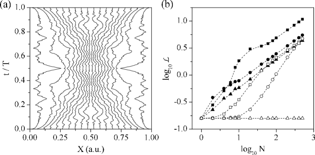
Figure 2: (a) QF–trajectories associated to a highly delocalized particle in a box. (b) Measure of the fractal dimension of a sample of QF–trajectories with initial positions: $x_{0}=0.01$ ($\blacksquare$), $x_{0}=0.1$ ($\bullet$), $x_{0}=0.4$ ($\blacktriangle$), $x_{0}=0.49$ ($\square$), $x_{0}=0.499$ ($\circ$), and $x_{0}=0.5$ ($\triangle$).

The complex space–time structure generated by $\rho_{t}$ along its evolution, the so–called fractal quantum carpet [13], can be easily understood by means of the QF–trajectories, which provide a causal description for such a pattern. As seen in figure 2(a), these trajectories manifest the symmetries displayed by $\Psi_{t}$, the guiding wave. Thus, in the case of the reflection symmetry with respect to $x_{c}$, the trajectories started at one side of the box (to the left or right of $x_{c}$) do not ever cross to the other side. This effect due to the single–valuedness of $S_{t}$, which avoids the trajectories to cross at the same time, can be compared with a hard–wall scattering problem; an ensemble of particles initially moving towards the wall will display similar features to those observed in figure 2(a) (see, for example, [14, 15]). Here, the particles cannot cross the point $x_{c}$, acting like a fictitious wall, and therefore they bounce backwards describing trajectories symmetric with respect to $t=T/2$. This inversion of the particle momentum is related to the second kind of symmetry that affects the wavefunction propagation: the change of sign of $S_{t}$ during the second half of the period. Moreover, unlike classical trajectories (and also caused by the single–valuedness of $S_{t}$), not all QF–trajectories can reach the wall, but will move parallel to it. This is a nice manifestation of the effects caused by the quantum pressure [1] under fractal conditions.

In figure 2(b), the logarithm of the length of several QF–trajectories, $\log_{10}\mathcal{L}$, is given as a function of $\log_{10}N$. As clearly seen, the converge to proportionality is faster for those QF–trajectories started at intermediate positions, between the boundary and the centre of the box. Notice also that, since the trajectory started at $x_{c}$ is not a fractal, its length does not depend on $N$. Independently of the initial position (and with the exception of the trajectory started at $x_{0}=0.5$), the fractal dimension of any trajectory asymptotically approaches the same value, $D_{f}\simeq 1.50$, which coincides with that found for $\rho_{t}$.

5 Causal considerations about the infiniteness of $\langle\hat{H}\rangle$

As seen in section 2, the expected value of the energy becomes infinite for quantum fractals. In the wavefunction (2), for example, the condition $2>s>0$ gives rise to a divergent series in $\langle\hat{H}\rangle$ when the limit (3) is taken into account. This property, unavoidable when dealing with quantum fractals, is related to their infinite scaling behaviour [8], which is lacking in (everywhere and anytime) regular wavefunctions. In the case of revivals of wavefunctions with discontinuities, like (20), which are regular only at certain times, $\langle\hat{H}\rangle$ also remains unbounded because an infinite number of eigenvectors is necessary to recreate the discontinuities. In this way, the discontinuities can be understood [6] as perturbations that propagate along the box in time, leading to the formation of the quantum fractals.

A more physical insight on the infiniteness of $\langle\hat{H}\rangle$ can be gained by appealing to the trajectory formulation introduced in section 3. In Bohmian mechanics, the particle energy is given by

$$E_{t}=\frac{(\nabla S_{t})^{2}}{2m}+V+Q_{t}.$$ (22)

Except in the case of particles associated to eigenvectors of the Hamiltonian, $E_{t}$ does not conserve in time in general, although the average energy of an ensemble of particles, initially distributed according to $\rho_{0}$,

$$\bar{E}=\int E_{t}\rho_{t}dx=\langle\hat{H}\rangle$$ (23)

does it, in agreement with the standard quantum mechanics. The classical analog of two couple particles can help to easily understand this fact; although the energy of each particle varies along time due to a continuous transfer between both, the total energy will remain constant. Therefore, though Bohmian particles are independent [12], the presence of the quantum potential in equation (14) leads to sort of non–local coupling or dependence between each particle and the rest from the ensemble (whose evolution is described by equation (13)).

In the example used in section 4 the potential energy is $V=0$ at any time. Thus, the initial total energy of almost all particles is zero, since they are distributed according to a constant probability density ($Q_{0}=0$) and the wavefunction is real ($S_{0}=0$). Only at the boundaries of the box $Q_{0}=\infty$ due to the discontinuity. This infinite amount of energy is stored up in the particles located at $x=\epsilon$ and $x=L-\epsilon$ with $\epsilon\to 0^{+}$, which constitute energy reservoirs. These energy reservoirs are the set of particles located at the discontinuities of $\Psi_{t}$ whenever a revival emerges, and not only at $t=0$.

The dynamical evolution of the system described by the wavefunction (20) can be explained in terms of this initial non–homogeneous energy distribution among particles as a function of their initial position. Although the particle distribution is homogeneous in space, the particles are not in quantum equilibrium, but subjected to an infinite gradient of energy at the boundaries of the box. This gradient leads to a strong, symmetric energy flow going from the boundaries towards the centre of the box that makes particles to move as shown in figure 2(a).

Figure 3: (a) Quantum trajectories associated to the wavefunction (20) with $N=3$. The total and kinetic energy, and the quantum potential are represented, respectively, in parts (b), (c) and (d) for three different trajectories of panel (a) with initial conditions: $x_{0}^{(1)}=0.01$ (thick solid line), $x_{0}^{(2)}=0.05$ (dashed line) and $x_{0}^{(3)}=0.3$ (dotted line). (e) Probability density at three different times: $t_{1}=0.15$ (dotted line), $t_{2}=0.35$ (dashed line) and $t_{3}=0.47$ (thick solid line), in units of $T$. These times are indicated in panel (a) by parallel, horizontal lines. The total and kinetic energy, and the quantum potential at these three times are represented, respectively, in parts (f), (g) and (h).

The relationship between the time dependence of the energy and the QF–trajectory dynamics can be better understood, without loss of generality, by recalling a simpler example consisting in assuming $N=3$ in the wavefunction (20). An ensemble of trajectories illustrating the dynamics associated with this case is shown in figure 3(a); these trajectories can be regarded as coarse–graining envelopes of the QF–trajectories shown above. Although the trajectories have not been distributed according to $\rho_{0}$, they provide an insight on how $\rho_{t}$ evolves, which is represented in figure 3(e) at three different times: $t_{1}=0.15$ (dotted line), $t_{2}=0.35$ (dashed line), and $t_{3}=0.47$ (thick solid line), in units of $T$. The total and kinetic energy, and the quantum potential are represented, respectively, in figures 3(f)–(h) at these three times. On the other hand, these magnitudes are also respectively displayed as a function of time in figures 3(b)–(d) for three different trajectories with initial conditions: $x_{0}^{(1)}=0.01$ (thick solid line), $x_{0}^{(2)}=0.05$ (dashed line), and $x_{0}^{(3)}=0.3$ (dotted line). As seen, the total energy can be, alternatively, positive or negative along time since it does not conserve.

The quantum potential acting on a particle depends on the structure of $\rho_{t}$ at each position of the particle. Thus, local minima in $\rho_{t}$ translate into negative wells in $Q_{t}$ that particles avoid [16], moving towards regions with positive values of $Q_{t}$, or, at least, presenting local maxima. The most dramatic case occurs when $\rho_{t}$ has a node (see $\rho_{t}$ at $t_{3}$), manifested as a singularity in $Q_{t}$. The intense forces around these regions make particles to move extremely fast apart from them [17], provoking peaks in their kinetic energies, as seen in figure 3(g). This behaviour is not observed, however, for those wells that appear in the central region. As commented above, this is because the particle cannot cross the point $x_{c}$ in these cases, but keeps moving for a certain time close to it until the quantum pressure decreases sufficiently, and can move backwards.

In this way, at $t_{1}$ very few particles remain close to the borders of the box (the maxima of $Q_{t}$ are relatively narrow), and most of them move towards the maxima located around $x\simeq 0.3$ and $x\simeq 0.7$, as can be seen in figure 3(a). This gives rise to the two important peaks in $\rho_{t}$; see figure 3(e). At $t_{2}$, the marginal maxima occupy a wider extension, however they are relatively high in energy, and therefore most of the particle flow directs towards the central maxima. As a consequence, $\rho_{t}$ displays an important central maximum, and two secondary, marginal maxima; see figure 3(e). Finally, at $t_{3}$, as seen in figure 3(e), most of the particles are collected in the centre of the box, between $x\simeq 0.25$ and $x\simeq 0.75$, impelled by the strong forces around $x\simeq 0.16$ and $x\simeq 0.84$, respectively. Moreover, since $Q_{t}$ reaches high values at the borders, very few particles will remain in such regions.

According to this analysis, it is clear that the three kinetic energy curves shown in figure 3(g) display peaks on the minima of $Q_{t}$, as would happen in a classical situation. However, the transient trapping observed along $x_{c}$ has a purely quantum nature, since there is no physical (classical) potential that may contribute to it [14, 15]. By following the sequence $t_{1}$–$t_{2}$–$t_{3}$, one can see that $Q_{t}$ progressively increases at the borders and develops deep wells that confine the particles within the central part of the box. In other words, the quantum pressure increases from the borders of the box towards the centre, pushing the particles towards $x_{c}$, and obliging them to move along this point for some time (approximately, half a period).

Taking into account the ideas exposed above, the analysis of a single particle dynamics becomes much simpler. For example, as seen in figure 3(a), the trajectory $x_{t}^{(1)}$ is initially slightly pushed away, towards $x_{c}$, by $Q_{t}$ until it reaches a turning point, and then moves backwards. Because of this, two peaks are observed in its kinetic energy, the second smaller than the first because the particle does not turn back to the original position. The turning point, like in classical mechanics, is characterized by a zero value of $K_{t}$. The fact that $Q_{t}$ reaches its minimum at the turning point can be understood as an appearance of a non–crossing wall (similar to that at $x_{c}$) avoiding the particle to go beyond it. On the other hand, between $t/T=0.3$ and $t/T=0.7$, the particle remains on top of the plateau seen in figure 3(h), and it is almost at rest (there is only a very slight oscillation at about $t/T=0.5$). The same is analysis applicable to the trajectory $x_{t}^{(2)}$, although the changes in its velocity are much more relevant, mainly at about $t/T=0.5$, when the particle undergoes the strong force due to the singularity in $Q_{t}$. Finally, for the trajectory $x_{t}^{(3)}$ the double peak is only observed at half of its evolution unlike the two previous cases. This is because this particle does not reach any turning point during the first part of its evolution, but only a sudden force that pushes it towards $x_{c}$ in a fast manner. Once in the trapping region (with the highest quantum pressure) the particle oscillates, and finally undergoes another sharp forcing that separates it from the neighbourhood of $x_{c}$.

In the light of the previous analysis, one can conclude that the variation in time of the energy can be understood as a regulating mechanism that adjusts the particle motion in such a way that it results consistent with the evolution of the wavefunction. The discussion applied to the trajectories guided by a three–state wavefunction also remains valid in the case of QF–trajectories. However, the motion adjustment takes place in a relatively faster manner, since particles will reach an infinite amount of turning points along their time evolution. Therefore, $Q_{t}$ and $K_{t}$ will display very deep wells and very sharp peaks, respectively, and the total (average) energy, given by equation (23), will diverge.

6 Conclusions

The consistent picture of quantum motion provided by Bohmian mechanics relies on a translation of the physics contained within the Schrödinger equation into a classical–like theory of motion. This transformation from one theory to the other is based on the regularity or differentiability of wavefunctions. Therefore, it does not hold for quantum fractals, non–regular solutions of the Schrödinger equation. A priori, this seems to be a failure of Bohmian mechanics in providing a complete explanation of quantum phenomena, since quantum fractals would not have a trajectory–based representation within its framework [5]. However, taking into account the fact that Bohmian mechanics is formally equivalent to the standard quantum mechanics, this incompleteness results quite “suspicious”.

By carefully studying the nature of quantum fractals, one can understand the source of such an incompatibility. These wavefunctions obey the Schrödinger equation in a weak sense [8], i.e., given the wavefunction as a linear superposition of eigenvectors of the Hamiltonian, the Schrödinger equation is satisfied by each eigenvector, but not by the wavefunction as a whole. This is because the eigenvectors are always continuous and differentiable everywhere, unlike quantum fractals, which are continuous everywhere, but differentiable nowhere. Taking this into account, a convenient way to express any arbitrary wavefunction, regular or fractal, is in terms of a superposition of eigenvectors of the Hamiltonian. This procedure is particularly important in those circumstances where the differentiability of the wavefunction is going to be invoked, like in the formulation of trajectory–based quantum theories like Bohmian mechanics.

In order to have a truly consistent particle equation of motion, Bohmian mechanics must be then reformulated in terms of an eigenvector decomposition of the wavefunction instead of considering the latter as a whole (as happens in standard Bohmian mechanics). The resulting generalized equation of motion, defined by a (convergent) limiting process, is valid for any arbitrary wavefunction, and provides the correct Bohmian trajectories. In the case of quantum fractals, one obtains the desired trajectory–based picture at the corresponding limit. Whereas, if the wavefunction is regular, the trajectories determined by means of this procedure will coincide with those given by the standard Bohmian equation of motion. This novel generalization thus proves the formal and physical completeness of Bohmian mechanics as a trajectory–based approach to quantum mechanics.

The trajectories associated to quantum fractals are also fractal. This explains both the formation of fractal quantum carpets and the unbounded expected value of the energy for quantum fractals. Although the example of a particle in a box has been used here to illustrate the peculiarities of quantum fractals, the analysis can be straightforwardly extended to continuum states [5] or other trajectory–based approaches to quantum mechanics, like Nelson’s theory of quantum Brownian motion [18]. Moreover, this kind of analysis can be of practical interest in the study of properties related to realistic systems, like those suggested by Wócik et al. [8] and Amanatidis et al. [9], providing moreover a causal insight on their physics.

Acknowledgments

The author gratefully acknowledges Prof. P. Brumer for his support during the preparation of this work, and Dr. M. J. W. Hall for interesting discussions on the problem posed here.

References

- [1] See, for example: Guantes R, Sanz A S, Margalef–Roig J and Miret–Artés S 2004 Surf. Sci. Rep. 53 199, and references therein.
- [2] Bohm D 1952 Phys. Rev. 85 166, 180
- [3] Dürr D, Goldstein S and Zanghì N 1992 J. Stat. Phys. 67 843
- [4] Holland P R 1993 The Quantum Theory of Motion (Cambridge: Cambridge University Press)
- [5] Hall M J W 2004 J. Phys. A 37 9549 (Hall M J W 2004 Preprint quant-ph/0406054)
- [6] Berry M V 1996 J. Phys. A 29 6617
- [7] Hall M J W, Reineker M S and Schleich W P 1999 J. Phys. A 32 8275
- [8] Wójcik D, Bialynicki–Birula I and Zyczkowski K 2000 Phys. Rev. Lett. 85 5022
- [9] Amanatidis E J, Katsanos D E and Evangelou S N 2004 Phys. Rev. B 69 195107
- [10] Mandelbrot B 1982 The Fractal Geometry of Nature (Freeman: San Francisco)
- [11] Strictly speaking, the wave function (3) is a semifractal [8] or prefractal [10], since it is derived from a convergent series. Prefractals are characterized by having a fractal first derivative.
- [12] In Bohmian mechanics each state is associated to one single particle. However, in agreement to the statistical postulate of the standard quantum mechanics, this particle can have any initial position with probability . Sampling all these initial positions one reproduces the results given by the standard quantum mechanics. This is equivalent to consider a system constituted by many non–interacting particles associated to the same wave function, and distributed according to .
- [13] The concept of fractal quantum carpet [8] arises from the term quantum carpet, which describes the (+1)–dimensional spacetime patterns generated by (regular) wave functions due to interference (see: Kaplan A E, Stifter P, van Leeuwen K A H, Lamb W E (Jr) and Schleich W P 1998 Phys. Scr. T76 93)
- [14] Sanz A S, Borondo F and Miret–Artés S 2004 J. Chem. Phys. 120 8794
- [15] Sanz A S and Miret–Artés S 2005 J. Chem. Phys. 122 14702
- [16] Sanz A S, Borondo F and Miret–Artés S 2000 Phys. Rev. B 61 7743
- [17] In the case of punctual nodes in high–dimensional problems, a vortical dynamics appear [14], and the particle can get trapped around the quantum vortex temporarily.
- [18] Nelson E 1966 Phys. Rev. 150 1079