Experimental Test of the Kochen-Specker Theorem for Single Qubits using Positive Operator-Valued Measures

Abstract

We present an experimental scheme for the implementation of arbitrary generalized measurements, represented by positive-operator valued measures, on the polarization of single photons, using linear optical devices. Further, we experimentally test a Kochen-Specker theorem for single qubits using positive operator-valued measures. Our experimental results for the first time disprove non-contextual hidden-variable theories, even for single qubits.

Hidden-variable theories (HV), inspired by Einstein, Podolsky, and Rosen (EPR) with their famous paradox r1 , has attracted broad interests. In 1960’s, Bell published his famous inequality r2 that revealed the quantitative contradiction between local hidden-variable (LHV) theories and quantum mechanics (QM), leading to experimental tests on this fundamental problem. A number of experiments r3 have observed the incompatibilities of LHV theories and experimental data, confirming that only by QM can the experimental results be correctly explained. There is another type, in fact a general type, of hidden-variable theories, i.e. the noncontextual hidden-variable (NCHV) theories. In such theories, values of physical observables are the same whatever the experimental context in which they appear. Kochen-Specker (KS) theorem r4 dictates the contradiction between such NCHV theories and QM. Recently, an all-or-nothing–type Kochen-Specker theorem has been experimentally tested r5 . Traditional KS theorem applies only to physical systems described by Hilbert spaces of dimension three or higher. However, it has been proved that KS theorems can be proved for a single two-level system (a qubit) cabello , using generalized measurements represented by positive operator-valued measures (POVMs) book1 ; book2 , which have found applications in various fields of physical research r6 ; cabello .

In this paper, we present an experimental scheme for implementation of arbitrary generalized measurements on polarization states of single photons, using linear optical devices. One interesting and important application is to experimentally test the Kochen-Specker (KS) theorem for a single qubit using POVMs cabello , as will be presented in this paper. We believe this is the first experimental test of a KS theorem for single qubits. Our results show that even for a single qubit NCHV theories cannot be consistent with experiments.

The POVM elements can always be expressed as linear combinations of one-dimensional operators, each of that has one and only one non-zero eigenvalue. Therefore it is sufficient davies to consider POVMs that consist all of one-dimensional operators. Based on the Neumark’s theorem neumark , it can be proved that either a $2\mathcal{N}$- or a $(2\mathcal{N}-1)$-element POVM in $\mathbb{C}^{2}$ can be realized via some orthogonal measurement (OM) in a $2\mathcal{N}$-dimensional Hilbert space $\mathbb{C}^{\mathcal{N}}\otimes\mathbb{C}^{2}$. First, we consider the POVM associated with the $2\mathcal{N}$-element set $\{E_{d}\}$ ($d=1,\cdots,2\mathcal{N}$) of the form

$$E_{d}=|\widetilde{\psi}_{d}\rangle\langle\widetilde{\psi}_{d}|,$$ (1)

where $|\widetilde{\psi}_{d}\rangle\in\mathbb{C}^{2}$ (not normalized) and $\sum_{d}E_{d}=I$ (the identity), there always exist vectors $|\widetilde{\phi}_{d}\rangle$ such that the following vectors

$$|\varphi_{d}\rangle=\left(\begin{array}[c]{c}|\widetilde{\psi}_{d}\rangle\\ |\widetilde{\phi}_{d}\rangle\end{array}\right)\in\mathbb{C}^{\mathcal{N}}\otimes\mathbb{C}^{2}$$ (2)

are orthonormal. The set $\{|\varphi_{d}\rangle\langle\varphi_{d}|\}$ thus represents the OM in $\mathbb{C}^{\mathcal{N}}\otimes\mathbb{C}^{2}$ that realizes the POVM $\{E_{d}\}$ in $\mathbb{C}^{2}$. The POVM $\{E_{d}\}$ on the state

$$|\Psi\rangle=\left(\begin{array}[c]{c}\alpha\\ \beta\end{array}\right)\in\mathbb{C}^{2}\ \left(|\alpha|^{2}+|\beta|^{2}=1\right)$$ (3)

can then be realized via the OM $\{|\varphi_{d}\rangle\langle\varphi_{d}|\}$ on the state

$$|\Phi\rangle=\left(\alpha,\beta,0,\cdots,0\right)^{Transpose}\in\mathbb{C}^{\mathcal{N}}\otimes\mathbb{C}^{2}.$$ (4)

Now consider the POVM associated with a $(2\mathcal{N}-1)$-element set $\{E_{d}^{\prime}\}$ ($d=1,\cdots,2\mathcal{N}-1$) of the form similar to Eq. (1):

$$E_{d}^{\prime}=|\widetilde{\psi}_{d}^{\prime}\rangle\langle\widetilde{\psi}_{d}^{\prime}|.$$ (5)

There also exist vectors $|\widetilde{\phi}_{d}^{\prime}\rangle$ such that the following $2\mathcal{N}$ vectors

$$|\varphi_{d}\rangle=\left(\begin{array}[c]{c}|\widetilde{\psi}_{d}^{\prime}\rangle\\ |\widetilde{\phi}_{d}^{\prime}\rangle\\ 0\end{array}\right),\qquad|\varphi_{2\mathcal{N}}\rangle=\left(\begin{array}[c]{c}0\\ \vdots\\ 0\\ 1\end{array}\right)\in\mathbb{C}^{\mathcal{N}}\otimes\mathbb{C}^{2},$$ (6)

are orthonormal. Hence the POVM $\{E_{d}^{\prime}\}$ on the state $|\Psi\rangle$ in Eq. (3) could be realized via the OM $\{|\varphi_{d}\rangle\langle\varphi_{d}|,|\varphi_{2\mathcal{N}}\rangle\langle\varphi_{2\mathcal{N}}|\}$ on the state $|\Phi\rangle$ in Eq. (4). Here we shall note that since $\langle\varphi_{2\mathcal{N}}|\Phi\rangle=0$, the projector $|\varphi_{2\mathcal{N}}\rangle\langle\varphi_{2\mathcal{N}}|$ will always yield null outcome when measuring the state $|\Phi\rangle$. Only the projectors $\{|\varphi_{d}\rangle\langle\varphi_{d}|\}$ could yield non-null outcomes, precisely corresponding to the POVM $\{E_{d}^{\prime}\}$.

For POVMs on the polarization states of a single photon, $\mathcal{N}$ different paths could be used to span the ancilla Hilbert space $\mathbb{C}^{\mathcal{N}}$. We denote them by mode states $|k\rangle$ ($k=1,\cdots,\mathcal{N}$). States $|\Psi\rangle$ in Eq. (3) and $|\Phi\rangle$ in Eq. (4) could thus be written as

$$|\Psi\rangle =\alpha|\text{H}\rangle+\beta|\text{V}\rangle,$$ (7)

$$|\Phi\rangle =|1\rangle\otimes\left(\alpha|\text{H}\rangle+\beta|\text{V}\rangle\right).$$ (8)

where $|\text{H}\rangle$ ($|\text{V}\rangle$) denotes the horizontal (vertical) polarization. The crucial step is then to perform the OM given in Eq. (2) or (6) on $|\Phi\rangle$.

Indeed, one can always find a $2\mathcal{N}$-dimensional unitary operator, say $U_{2\mathcal{N}}$, that fulfills exactly the following transformation,

$$|\varphi_{2k-1}\rangle\ ^{\underrightarrow{\ U_{2\mathcal{N}}\ }}\ |k,\text{H}\rangle,\qquad|\varphi_{2k}\rangle\ ^{\underrightarrow{\ U_{2\mathcal{N}}\ }}\ |k,\text{V}\rangle,$$ (9)

with $k=1,\cdots,\mathcal{N}$ and $|k,\text{H}\rangle=|k\rangle\otimes|\text{H}\rangle$ etc. Therefore the OM on the state $|1\rangle\otimes\left(\alpha|\text{H}\rangle+\beta|\text{V}\rangle\right)$, and consequently POVM $\{E_{d}\}$ on $\alpha|\text{H}\rangle+\beta|\text{V}\rangle$, can be realized by performing OM $\{|k,\text{H}\rangle\langle k,\text{H}|,|k,\text{V}\rangle\langle k,\text{V}|\}$ on $U_{2\mathcal{N}}\left[|1\rangle\otimes\left(a|\text{H}\rangle+b|\text{V}\rangle\right)\right]$. It is obvious that OM $\{|k,\text{H}\rangle\langle k,\text{H}|,|k,\text{V}\rangle\langle k,\text{V}|\}$ can be carried out by placing polarizing beam splitters (PBS) followed by single-photon detectors at out-ports of every path. In what follows, we describe the scheme for implementing arbitrary unitary operators on the Hilbert space $\mathbb{C}^{\mathcal{N}}\otimes\mathbb{C}^{2}$, of which $\mathbb{C}^{\mathcal{N}}$ is spanned by paths while $\mathbb{C}^{2}$ by polarization.

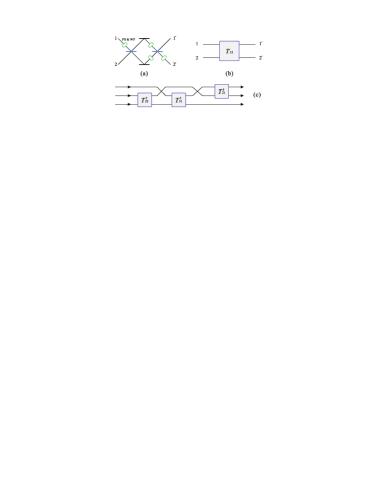
Figure 1: (a) A Mach-Zehnder interferometer with properly placed phase shifters and wave plates (PS&WP’s) can be used as the basic building block of any $2N$-dimensional unitary matrix. The Mach-Zehnder interferometer can be represented by the abstract four-port device in (b). (c) Three Mach-Zehnder interferometer devices $T_{pq}$ are enough to build any unitary operators on $\mathbb{C}^{3}\otimes\mathbb{C}^{2}$.

The technique employed here is similar as in Ref. reck . As shown in Ref. eng , the most general element of $U\left(4\right)$ can be realized by a Mach-Zehnder (MZ) interferometer with four specific unitary operation on the polarization, which could be realized by a proper combination of phase shifters, quarter- and half-wave plates [see in Fig. 1(a)]. The most crucial observation is that an arbitrary $2\mathcal{N}$-dimensional unitary operator can be factorized into a product of block matrices which can be realized by a $U\left(4\right)$ operation on the Hilbert space spanned by the polarizations and two different paths.

We define a matrix $T_{pq}$ ($p,q=1,\cdots,\mathcal{N}$) which is a $2\mathcal{N}$-dimensional identity matrix with the elements $I_{ij}$ ($i=2p-1,2p;j=2q-1,2q$) replaced by corresponding elements of the $U\left(4\right)$ operator of a MZ as in Fig. 1(a,b). Using methods similar to Gaussian elimination, by being multiplied from the right with a succession of MZ $T_{\mathcal{N},q}$ ($q=\mathcal{N}-1,\cdots,1$), a $2\mathcal{N}$-dimensional unitary operator $U_{2\mathcal{N}}$ can be reduced into a direct sum of a $\left(2\mathcal{N}-2\right)$-dimensional unitary operator $U_{2\mathcal{N}-2}$ and the $2$-dimensional identity operator $I_{2}$:

$$U_{2\mathcal{N}}\cdot T_{\mathcal{N},\mathcal{N}-1}\cdot T_{\mathcal{N},\mathcal{N}-2}\cdot\cdots\cdot T_{\mathcal{N},1}=\left(\begin{array}[c]{cc}U_{2\mathcal{N}-2}&0\\ 0&I_{2}\end{array}\right).$$ (10)

The sequence of MZ transformations can be applied recursively to the matrix with reduced dimensions. Thus we can make the resulting matrix equal to the identity,

$$U_{2\mathcal{N}}\cdot T_{\mathcal{N},\mathcal{N}-1}\cdot T_{\mathcal{N},\mathcal{N}-2}\cdots\cdot T_{2,1}=I_{2\mathcal{N}},$$ (11)

and consequently we have

$$U_{2\mathcal{N}} =\left(T_{\mathcal{N},\mathcal{N}-1}\cdot T_{\mathcal{N},\mathcal{N}-2}\cdot\cdots\cdot T_{2,1}\right)^{-1}$$

$$=T_{2,1}^{{\dagger}}\cdot\cdots\cdot T_{\mathcal{N},\mathcal{N}-2}^{{\dagger}}\cdot T_{\mathcal{N},\mathcal{N}-1}^{{\dagger}}.$$ (12)

Therefore the unitary transformation $U_{2\mathcal{N}}$ could be realized by recursively placing proper MZs shown in Fig. 1(a). As an example, we present in Fig. 1(c) the setup for a general unitary matrix on $\mathbb{C}^{3}\otimes\mathbb{C}^{2}$. We shall note that our scheme is similar to the one proposed in Ref. reck , where however the polarization was not involved. Once all unitary transformations on $\mathbb{C}^{\mathcal{N}}\otimes\mathbb{C}^{2}$ becomes realizable, it is possible to perform any POVM on the polarization states of single photons. For the task of performing a POVM on the polarization states of single photons, the full setup according to Eq. (12) contains MZs of which the inputs and outputs are exactly vacuum states. These MZs can be simply removed [e.g. the $T_{32}^{{\dagger}}$ in Fig. 1(c)], and the setup of the POVM can hence be further simplified.

One of the applications of the above scheme is to the optical test of a KS theorem for a single qubit using positive operator-valued measures, proposed by M. Nakamura (see Ref. [28] of cabello ). We now briefly describe the KS theorem tested in this paper, which is in fact a simpler version of the one proved in Ref. cabello .

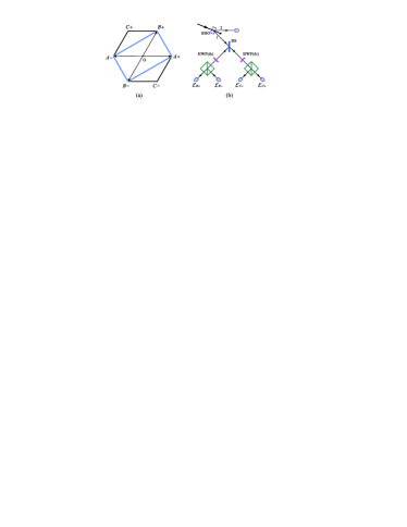
Figure 2: (a) Notation for the six vertices of the regular hexagon: $A+$ is the antipode of $A-$, etc. $O$ is the center of the regular hexagon. The rectangle formed by $A\pm$ and $B\pm$ is one of the three inscribed (sharing vertices) in the regular hexagon. It corresponds to the four-element POVM $\{\mathcal{E}_{A\pm},\mathcal{E}_{B\pm}\}$. (b) The schematic setup for the realization of the POVM $\{\mathcal{E}_{B\pm},\mathcal{E}_{C\pm}\}$. The beam splitter is a 50:50 one. The two half-wave plates are set at $\theta_{B}=15{{}^{\circ}}$ and $\theta_{C}=30{{}^{\circ}}$.

Let $A$, $B$, $C$ be the three directions obtained by joining the center of a regular hexagon with its three non-antipodal vertices, as illustrated in Fig. 2(a). We can define six positive-semidefinite operators, $\{\mathcal{E}_{A\pm},\mathcal{E}_{B\pm},\mathcal{E}_{C\pm}\}$, as follows.

$$\mathcal{E}_{A\pm} =\frac{1}{2}\left|A\pm\right\rangle\left\langle A\pm\right|,\qquad\mathcal{E}_{B\pm}=\frac{1}{2}\left|B\pm\right\rangle\left\langle B\pm\right|,$$

$$\mathcal{E}_{C\pm} =\frac{1}{2}\left|C\pm\right\rangle\left\langle C\pm\right|.$$ (13)

These six operators can be used to construct three four-element POVMs:

$$\{\mathcal{E}_{A\pm},\mathcal{E}_{B\pm}\},\qquad\{\mathcal{E}_{B\pm},\mathcal{E}_{C\pm}\},\qquad\{\mathcal{E}_{C\pm},\mathcal{E}_{A\pm}\}.$$ (14)

Geometrically, as shown in Fig. 2(a), there are only three rectangles share inscribed (sharing vertices) in a regular hexagon. All of them share the same center, and any two rectangles share two antipodal vertices. Each rectangle allows us to define a four-element POVM, which can be expressed as

$$\mathcal{E}_{A+}+\mathcal{E}_{B+}+\mathcal{E}_{A-}+\mathcal{E}_{B-} =I_{2},$$

$$\mathcal{E}_{B+}+\mathcal{E}_{C+}+\mathcal{E}_{B-}+\mathcal{E}_{C-} =I_{2},$$

$$\mathcal{E}_{C+}+\mathcal{E}_{A+}+\mathcal{E}_{C-}+\mathcal{E}_{A-} =I_{2}.$$ (15)

Each equation contains four positive-semidefinite operators, summing up to the identity. A NCHV theory must assign the answer yes to one and only one of these four operators. However, such an assignment is impossible, since each operator appears twice in Eqs. (15), so that the total number of yes answers must be an even number, while the number of possible yes answers, is three.

Experimentally, a qubit can be represented by polarization of a single photon. In the basis of horizontal polarization $|\text{H}\rangle$ and vertical polarization $\left|\text{V}\right\rangle$, we can write,

$$\begin{array}[c]{ll}|A+\rangle=|\text{H}\rangle,&|A-\rangle=|\text{V}\rangle,\\ |B+\rangle=\frac{\sqrt{3}}{2}|\text{H}\rangle+\frac{1}{2}|\text{V}\rangle,&|B-\rangle=\frac{1}{2}|\text{H}\rangle-\frac{\sqrt{3}}{2}|\text{V}\rangle,\\ |C+\rangle=\frac{1}{2}|\text{H}\rangle+\frac{\sqrt{3}}{2}|\text{V}\rangle,&|C-\rangle=\frac{\sqrt{3}}{2}|\text{H}\rangle-\frac{1}{2}|\text{V}\rangle.\end{array}$$ (16)

Taking the implementation of the POVM $\{\mathcal{E}_{B\pm},\mathcal{E}_{C\pm}\}$ as an example, the corresponding OM can be constructed with the following four orthonormal states in $\mathbb{C}^{2}\otimes\mathbb{C}^{2}$ [see Eq. (2)]:

$$\frac{1}{\sqrt{2}}\begin{pmatrix}|B\pm\rangle\\ i|B\pm\rangle\end{pmatrix} =\frac{|1\rangle+i|2\rangle}{\sqrt{2}}\otimes|B\pm\rangle,$$

$$\frac{1}{\sqrt{2}}\begin{pmatrix}|C\pm\rangle\\ -i|C\pm\rangle\end{pmatrix} =\frac{|1\rangle-i|2\rangle}{\sqrt{2}}\otimes|C\pm\rangle.$$ (17)

Due to the specific form of Eqs. (17), the unitary transformation shown in Eq. (9) can be realized simply by a single 50:50 beam splitter (BS) followed by two unitary transformations on the polarization states, without the necessity of a full setup of the MZ shown in Fig. 1(a). To be specific, the BS (with properly defined phase shifts) realizes transformation

$$\frac{|1\rangle+i|2\rangle}{\sqrt{2}}\rightarrow|1\rangle,\qquad\frac{|1\rangle-i|2\rangle}{\sqrt{2}}\rightarrow|2\rangle,$$ (18)

The two unitary transformations on the polarization states are designed to be

$$U_{B}=\left(\begin{array}[c]{cc}\frac{\sqrt{3}}{2}&\frac{1}{2}\\ \frac{1}{2}&-\frac{\sqrt{3}}{2}\end{array}\right),\qquad U_{C}=\left(\begin{array}[c]{cc}\frac{1}{2}&\frac{\sqrt{3}}{2}\\ \frac{\sqrt{3}}{2}&-\frac{1}{2}\end{array}\right),$$ (19)

which realize transformation

$$U_{B}|B+\rangle =U_{C}|C+\rangle=|\text{H}\rangle,$$

$$U_{B}|B-\rangle =U_{C}|C-\rangle=|\text{V}\rangle.$$ (20)

Hence the unitary transformation shown in Eq. (9) for this case is realized.

According to Ref. eng , $U_{B}$, and $U_{C}$ could be realized by only half-wave plates (HWP). The HWP, with its major axis at an angle $\theta$ to the vertical direction, is accounted for the unitary operator (up to an overall phase factor)

$$\text{HWP}\left(\theta\right)=\left(\begin{array}[c]{cc}\cos 2\theta&\sin 2\theta\\ \sin 2\theta&-\cos 2\theta\end{array}\right).$$ (21)

Therefore we have

$$U_{B}=\text{HWP}\left(\theta_{B}\right),\qquad U_{C}=\text{HWP}\left(\theta_{C}\right),$$ (22)

with

$$\theta_{B}=\frac{1}{2}\arccos\frac{\sqrt{3}}{2}=15{{}^{\circ}},\qquad\theta_{C}=\frac{1}{2}\arccos\frac{1}{2}=30{{}^{\circ}}.$$ (23)

The schematic drawing of the implementation of POVM $\{\mathcal{E}_{B\pm},\mathcal{E}_{C\pm}\}$ is shown in Fig. 2(b). The POVM $\{\mathcal{E}_{A\pm},\mathcal{E}_{B\pm}\}$ ($\{\mathcal{E}_{C\pm},\mathcal{E}_{A\pm}\}$) could be implemented by simply removing HWP$\left(\theta_{C}\right)$ [HWP$\left(\theta_{B}\right)$] in Fig. 2(b), with the detectors that previously corresponds to $\mathcal{E}_{C\pm}$ ($\mathcal{E}_{B\pm}$) now corresponding to $\mathcal{E}_{A\pm}$.

Table 1: The experimental data counted in $10$ seconds. For each POVM, “1-fold counts” shows the counts that only one operator yields the answer yes with coincidence with the detector of photon $2$, while “2-fold counts” means that two operators simultaneously yield answer yes with coincidence with the detector of photon $2$. The data in “2-fold counts” has been scaled according to the carefully measured efficiency of our single photon detectors and is hence comparable with data in “1-fold counts”. In our experiments, the 3- and 4-fold coincidence counts, corresponding to that more than two operators yield the answer yes, turn out to be virtually zero in $10$ seconds.

$\{\mu_{\pm},\nu_{\pm}\}$		1-fold counts				2-fold counts
$\mu$	$\nu$	$\mu_{+}$	$\mu_{-}$	$\nu_{+}$	$\nu_{-}$	$\begin{array}[]{c}\mu_{+}\\ \nu_{+}\end{array}$	$\begin{array}[]{c}\mu_{+}\\ \nu_{-}\end{array}$	$\begin{array}[]{c}\mu_{-}\\ \nu_{+}\end{array}$	$\begin{array}[]{c}\mu_{-}\\ \nu_{-}\end{array}$
$\mathcal{E}_{A}$	$\mathcal{E}_{B}$	$14718$	$10474$	$13156$	$12587$	$34$	$69$	$38$	$40$
$\mathcal{E}_{B}$	$\mathcal{E}_{C}$	$10660$	$14781$	$11902$	$12103$	$95$	$47$	$85$	$63$
$\mathcal{E}_{C}$	$\mathcal{E}_{A}$	$12883$	$10586$	$13764$	$10940$	$128$	$39$	$18$	$24$

Here we shall note that although our experiment and that in Ref. r5 are both based on single photons, there are substantial differences. In theory, our experiment tests the KS theorem for a single two-level system. The path degrees of freedom are used as ancilla, which according to Ref. cabello should be regarded as part of the measurement apparatus, which can be considered to arise from the beam splitter-induced “interference” between the photon to be measured and the vacuum. While in Ref. r5 the path degrees of freedom are part of the system to be tested. In practice, our experiment does not demand the full MZ setup, and is irrelevant to relative phases between paths. Hence our experiment is much simpler and more convenient.

In experiments, we generate two photons (labelled by $1$ and $2$) in the maximally entangled state, with a visibility of about $82\%$, $|\Psi^{-}\rangle_{12}=\frac{1}{\sqrt{2}}\left(|\text{H}\rangle_{1}|\text{V}\rangle_{2}-|\text{V}\rangle_{1}|\text{H}\rangle_{2}\right)$ by type-II spontaneous parametric down conversion (SPDC) from a pump pulse passing through a beta-barium borate (BBO) crystal. The UV laser with a central wavelength of $394$nm has a pulse duration of $80$fs, a repetition rate of $80$MHz, and an average power of $110$mw. By tracing out photon $2$, photon $1$ is left in a maximal mixed state described by density matrix $\rho_{1}=\frac{1}{2}\left(|\text{H}\rangle\langle\text{H}|+|\text{V}\rangle\langle\text{V}|\right).$ The three POVMs, $\{\mathcal{E}_{A\pm},\mathcal{E}_{B\pm}\}$, $\{\mathcal{E}_{B\pm},\mathcal{E}_{C\pm}\}$, and $\{\mathcal{E}_{C\pm},\mathcal{E}_{A\pm}\}$, are performed on photon $1$ at state $\rho_{1}$.

The experimental data contained in Table 1 shows the number of the events in which one and only one operator yields the answer yes, and the number of those in which more than one operator simultaneously yield the answer yes. The collection and detection efficiencies of the four port are $\sim 5\%$ in our experiments. Through careful calculation, the 2-fold coincidence has been scaled to be comparable to 1-fold data and the experimental results coincide with a very high precision ($\sim 99\%$) with Eqs. (15), which therefore experimentally excludes the existence of a non-contextual hidden-variable theory even for a single qubit. From the experimental point of view, these 2-fold counts are due to the imperfect entangled photon source. In our experiments, because of the probablistic feature of pair creation in SPDC, there will be a small probability that more than one pair is generated. The additional pair(s) will give some 2-fold counts (about $150$), which is of the same order of the counts observed in our experiments as presented in Table 1.

In conclusion, we propose an experimental scheme for the implementation of arbitrary positive operator-valued measures on the polarization states of single photons using linear optical devices. This scheme may have various applications in quantum information processing. As a demonstration, we present the experimental test of the KS theorem for a single qubit using POVM. Our experiment verifies with very good precision that even a single qubit could not be described by NCHV theory.

We thank Z.B. Chen for fruitful discussions and valuable suggestions. This work was supported by the Nature Science Foundation of China, the Chinese Academy of Sciences, and the National Fundamental Research Program (under Grant No. 2001CB309300).

References

(1)A. Einstein, B. Podolsky, and N. Rosen, Phys. Rev. 47,
777 (1935).
(2)J. S. Bell, Rev. Mod. Phys. 38, 447 (1966).
(3)A. Aspect et al., Phys. Rev. Lett. 49, 1804 (1982); Y.H.
Shih and C.O. Alley, Phys. Rev. Lett. 61, 2921 (1988);
J.-W. Pan et al., Nature (London) 403, 515 (2000); Zhi
Zhao et al., Phys. Rev. Lett. 91, 180401 (2003).
(4)S. Kochen and E.P. Specker, J. Math. Mech. 17, 59 (1967).
(5)Y.F. Huang et al., Phys. Rev. Lett. 90, 250401 (2003).
(6)A. Cabello, Phys. Rev. Lett. 90, 190401 (2003).
(7)P. Busch et al., Operational Quantum Physics
(Springer-Verlag, Berlin Heidelberg, 1995).