Transmission of ultracold atoms through a micromaser : detuning effects

Abstract

The transmission probability of ultracold atoms through a micromaser is studied in the general case where a detuning between the cavity mode and the atomic transition frequencies is present. We generalize previous results established in the resonant case (zero detuning) for the mesa mode function. In particular, it is shown that the velocity selection of cold atoms passing through the micromaser can be very easily tuned and enhanced using a non-resonant field inside the cavity. Also, the transmission probability exhibits with respect to the detuning very sharp resonances that could define single cavity devices for high accuracy metrology purposes (atomic clocks).

I Introduction

Laser cooling of atoms has become these last years an interesting tool in atom optics (see e.g. Refs. Adams et al. (1994); Adams and Riis (1997) for a review of these topics). The production of slow atomic beams and the control of their motion by laser light has opened a variety of applications including matter-wave interferometers Kasevich and Chu (1991), atomic lenses or atom lithography Timp et al. (1992). In such experiments, it is often highly desirable to control actively the velocity distribution of an atomic ensemble. More particularly, devices for narrowing this distribution over a well fixed velocity are very useful to define an atomic beam with a long coherence length (like in atom lasers Ketterle (2002)). Velocity monochromatization of atomic beams making use of an optical cavity has already been suggested by Balykin Balykin (1989). For ultracold atoms, Löffler et al. Löffler et al. (1998) have recently proposed a velocity selector based on a 1D micromaser scheme (also referred to as mazer). They suggest to send a beam of cold atoms through a microwave cavity in resonance with one of the atomic transitions. The small velocity of the atoms at the entrance of the micromaser require to quantize their center-of-mass motion to describe correctly their interaction with the cavity quantum field (see e.g. Refs. Schleich (1997); Bastin and Martin (2003) for an overview of quantized motion in quantized fields). This quantization is an essential feature as it leads to a fundamental interplay between their motion and the atom-field internal state Scully et al. (1996). It results from this that most of the incoming atoms may be found reflected by the field present in the cavity, except at certain velocities where they can be transmitted through with a reasonable efficiency. At the exit of the cavity, the longitudinal velocity distribution of the cold atomic beam may be this way significantly narrowed Löffler et al. (1998) and a splitting of the atomic wave packet may be observed Bienert and Freyberger (2001). These effects have been first described by Haroche et al. Haroche et al. (1991), Englert et al. Englert et al. (1991) and Battocletti and Englert Battocletti and Englert (1994). They have been recently experimentally observed in the optical domain (see, for example, Pinkse et al. Pinske et al. (2000)).

In this paper, we extend the proposal of Löffler et al. Löffler et al. (1998) by considering an off-resonant interaction between the atoms and the cavity field. This case offers new attractive perspectives for metrology purposes and in the velocity selection scheme. Let us emphasize that this scheme is in no way a proposal to reduce the transverse momentum spread of an atomic beam. For applications where this point is important (like for example in the case of an atomic beam splitter based on Doppleron resonances Glasgow et al. (1991)), other schemes like quantum-nondemolition measurement of atomic momentum Sleator and Wilkens (1993) should rather be used.

II Transmission probability through the mazer

We consider two-level atoms moving along the $z$ direction on the way to a cavity of length $L$. The atoms are coupled off-resonantly to a single mode of the quantized field present in the cavity. The atomic center-of-mass motion is described quantum mechanically and the usual rotating-wave approximation is made. The Hamiltonian of the system reads

$$H=\hbar\omega_{0}\sigma^{\dagger}\sigma+\hbar\omega a^{\dagger}a+\frac{p^{2}}{2m}+\hbar gu(z)(a^{\dagger}\sigma+a\sigma^{\dagger}),$$ (1)

where $p$ is the atomic center-of-mass momentum along the $z$ axis, $m$ the atomic mass, $\omega_{0}$ the atomic transition frequency, $\omega$ the cavity field mode frequency, $\sigma=|b\rangle\langle a|$ ($|a\rangle$ and $|b\rangle$ are respectively the upper and lower levels of the two-level atom), $a$ and $a^{\dagger}$ are respectively the annihilation and creation operators of the cavity radiation field, $g$ is the atom-field coupling strength and $u(z)$ is the cavity field mode. We denote also hereafter $\kappa=\sqrt{2mg/\hbar}$, $\kappa_{n}=\kappa\sqrt[4]{n+1}$, $\delta$ the detuning $\omega-\omega_{0}$, and $\theta_{n}$ the angle defining the dressed-state basis given by

$$\cot 2\theta_{n}=-\frac{\delta}{\Omega_{n}}\,,$$ (2)

with $\Omega_{n}=2g\sqrt{n+1}$.

The properties of the mazer have been established in the resonant case by Scully and collaborators Meyer et al. (1997); Löffler et al. (1997); Schröder et al. (1997). We extended very recently these studies in the non-resonant case Bastin and Martin (2003), especially for the mesa mode function ($u(z)=1$ inside the cavity, 0 elsewhere). Particularly, we have shown that, if the cavity field is prepared in the Fock state $|n\rangle$, an atom initially in the excited state $|a\rangle$ with a momentum $\hbar k$ will be found transmitted by the cavity in the same state or in the lower state $|b\rangle$ with the respective probabilities

$$T^{a}_{n}(k)=|\tau^{a}_{n}(k)|^{2},$$ (3)

and

$$\qquad T^{b}_{n+1}(k)=\left\{\begin{array}[]{ll}\frac{k_{b}}{k}|\tau^{b}_{n+1}(k)|^{2}&\textrm{ if }\left(\frac{k}{\kappa}\right)^{2}>\frac{\delta}{g},\vspace{0.2cm}\\ 0&\textrm{ otherwise},\end{array}\right.$$ (4)

where

$$k^{2}_{b}=k^{2}-\kappa^{2}\frac{\delta}{g},$$ (5)

and

$$\tau^{a}_{n}(k) =\frac{\cos^{2}\theta_{n}\frac{\tau^{-}_{n}(k)}{\tau^{-}_{n}(k_{b})}\,\tau^{+}_{n}(k_{b})+\sin^{2}\theta_{n}\,{\tau^{-}_{n}(k)}}{\left(\cos^{2}\theta_{n}\frac{k-k_{b}}{k^{c}_{n}}-1\right)\left(\cos^{2}\theta_{n}\frac{k-k_{b}}{k^{t}_{n}}-1\right)},$$ (6)

$$\tau^{b}_{n+1}(k) =\frac{\sin 2\theta_{n}}{4}\left(1+\frac{k}{k_{b}}\right)$$

$$\;\;\times\frac{\frac{\tau^{-}_{n}(k)}{\tilde{\tau}^{-}_{n}(k,k_{b})}\,\tau^{+}_{n}(k_{b})-\frac{\tau^{+}_{n}(k_{b})}{\tilde{\tau}^{+}_{n}(k,k_{b})}\,\tau^{-}_{n}(k)}{\left(\cos^{2}\theta_{n}\frac{k-k_{b}}{k^{c}_{n}}-1\right)\left(\cos^{2}\theta_{n}\frac{k-k_{b}}{k^{t}_{n}}-1\right)},$$ (7)

with

$$\tau^{\pm}_{n}(k)=\left[\cos(k^{\pm}_{n}L)-i\Sigma^{\pm}_{n}(k)\sin(k^{\pm}_{n}L)\right]^{-1},$$ (8)

$$\tilde{\tau}^{\pm}_{n}(k,k_{b})=\left[\cos(k^{\pm}_{n}L)-i\tilde{\Sigma}^{\pm}_{n}(k,k_{b})\sin(k^{\pm}_{n}L)\right]^{-1},$$ (9)

$${k^{+}_{n}}^{2} =k^{2}-\kappa_{n}^{2}\tan\theta_{n},$$ (10)

$${k^{-}_{n}}^{2} =k^{2}+\kappa_{n}^{2}\cot\theta_{n},$$ (11)

$$\Sigma^{\pm}_{n}(k)=\frac{1}{2}\left(\frac{k^{\pm}_{n}}{k}+\frac{k}{k^{\pm}_{n}}\right),$$ (12)

$$\tilde{\Sigma}^{\pm}_{n}(k,k_{b})=\left(\frac{k^{\pm}_{n}}{k+k_{b}}+\frac{k_{b}}{k+k_{b}}\frac{k}{k^{\pm}_{n}}\right),$$ (13)

$$k^{c}_{n}=i\frac{\left(k+i\cot(\frac{k^{-}_{n}L}{2})k^{-}_{n}\right)\left(k_{b}+i\cot(\frac{k^{+}_{n}L}{2})k^{+}_{n}\right)}{\cot(\frac{k^{-}_{n}L}{2})k^{-}_{n}-\cot(\frac{k^{+}_{n}L}{2})k^{+}_{n}},$$ (14)

$$k^{t}_{n}=i\frac{\left(k-i\tan(\frac{k^{-}_{n}L}{2})k^{-}_{n}\right)\left(k_{b}-i\tan(\frac{k^{+}_{n}L}{2})k^{+}_{n}\right)}{\tan(\frac{k^{+}_{n}L}{2})k^{+}_{n}-\tan(\frac{k^{-}_{n}L}{2})k^{-}_{n}}.$$ (15)

The atom transmission in the lower state $|b\rangle$ results in a photon induced emission inside the cavity. In presence of a detuning, these atoms are found to propagate with a momentum $\hbar k_{b}$ different from the initial value $\hbar k$ (see Bastin and Martin (2003)). This results merely from the energy conservation. Contrary to the resonant case, the final state of the process $|b,n+1\rangle$ has an internal energy different from that of the initial one ($|a,n\rangle$). The energy difference $\hbar\delta$ is transferred to the atomic kinetic energy. According to the sign of the detuning, the atoms are either accelerated ($\delta<0$, heating process) or decelerated ($\delta>0$, cooling process). In this last case, the initial atomic kinetic energy ($\hbar^{2}k^{2}/2m$) must be greater than $\hbar\delta$ to ensure that the photon emission may occur. This justifies the conditional result in Eq. (4).

In the ultracold regime ($k\ll\kappa_{n}\sqrt{\tan\theta_{n}}$) and for $\exp(\kappa_{n}L)\gg 1$ we have $\tau^{+}_{n}(k)\simeq 0$ and the total transmission probability $T_{n}(k)=T^{a}_{n}(k)+T^{b}_{n+1}(k)$ simplifies to

$$\qquad T_{n}(k)=f(\theta_{n})\mathcal{I}(L)|\tau^{-}_{n}(k)|^{2}$$ (16)

with

$$f(\theta_{n})=\left\{\begin{array}[]{ll}\sin^{2}\theta_{n}(\sin^{2}\theta_{n}+\frac{k_{b}}{k}\cos^{2}\theta_{n})&\textrm{ if }\left(\frac{k}{\kappa}\right)^{2}>\frac{\delta}{g},\\ \sin^{4}\theta_{n}&\textrm{ otherwise}.\end{array}\right.$$ (17)

$$\mathcal{I}(L)=\frac{1}{\left|\cos^{2}\theta_{n}\frac{k-k_{b}}{k^{c}_{n}}-1\right|^{2}\left|\cos^{2}\theta_{n}\frac{k-k_{b}}{k^{t}_{n}}-1\right|^{2}},$$ (18)

and

$$|\tau^{-}_{n}(k)|^{2}\simeq\frac{1}{1+\left(\frac{\kappa_{n}}{2k}\right)^{2}\cot\theta_{n}\sin^{2}(k_{n}^{-}L)}.$$ (19)

At resonance ($\delta=0$), $k_{b}=k$, $\theta_{n}=\pi/4$ and Eq. (16) well reduces to the result of Löffler et al. Löffler et al. (1998)

$$T_{n}(k)=\frac{1}{2}|\tau^{-}_{n}(k)|^{2}=\frac{1}{2}\frac{1}{1+\left(\frac{\kappa_{n}}{2k}\right)^{2}\sin^{2}(k_{n}^{-}L)}.$$ (20)

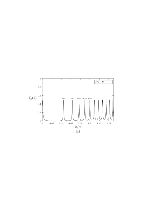
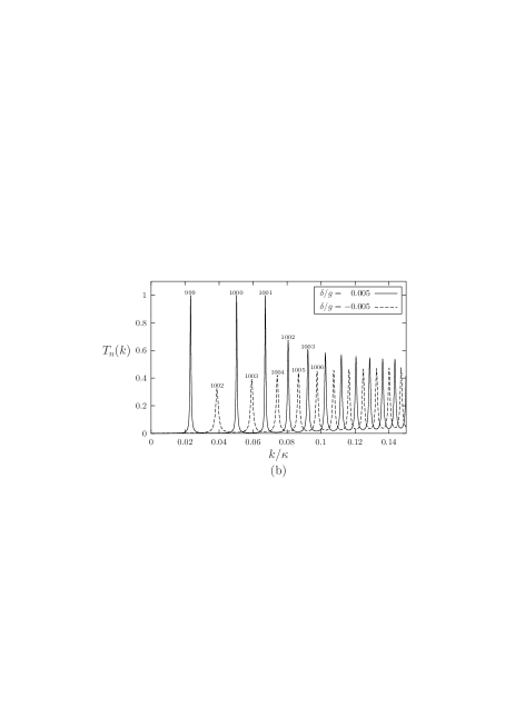
Figure 1: Transmission probability of an excited atom through the mazer with respect to $k/\kappa$. (a) $\delta/g=0$, (b) $\delta/g=\pm 0.005$. The interaction length was fixed to $\kappa L=10^{3}\pi$ and $n=0$.

We present on figs. 1 the transmission probability of an initially excited atom through the mazer. With respect to the wavenumber of the incoming atoms $k/\kappa_{n}$ or the interaction length $\kappa_{n}L$, the transmission probability $T$ shows various resonances. For $(k/\kappa)^{2}>\delta/g$, their position is given by

$$k_{n}^{-}L=m\pi\quad(m\textrm{ a positive integer}).$$ (21)

As the de Broglie wavelength is given in the ultracold regime by $\lambda_{\mathrm{dB}}=2\pi/k^{-}_{n}$, this occurs when the cavity length fits a multiple of half the de Broglie wavelength $\lambda_{\mathrm{dB}}$ of the atom inside the cavity :

$$L=m\frac{\lambda_{\mathrm{dB}}}{2}.$$ (22)

The position of the $m^{\textrm{th}}$ resonance in the $k$ space is therefore given by

$$\left.\frac{k}{\kappa}\right|_{m}=\sqrt{\left(\frac{m\pi}{\kappa L}\right)^{2}-\sqrt{n+1}\cot\theta_{n}}.$$ (23)

For $(k/\kappa)^{2}\leq\delta/g$, a careful analysis of the transmission probability (16) yields resonance positions slightly shifted from the values given by Eq. (21).

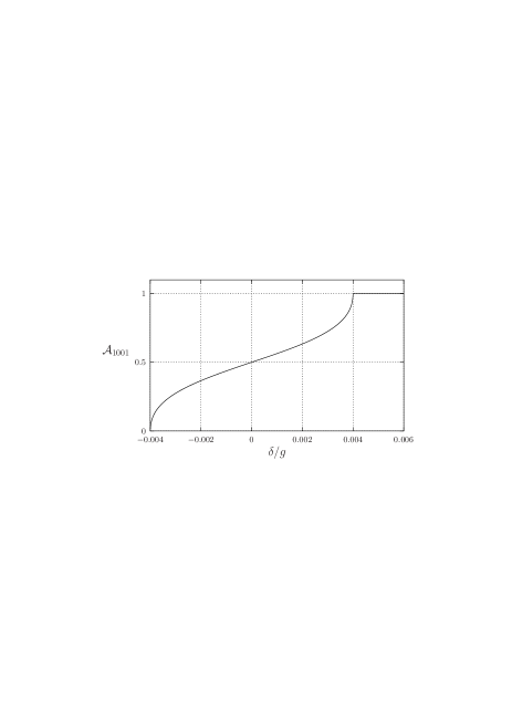
Figure 2: Amplitude of the $1001^{\textrm{st}}$ resonance with respect to the detuning value ($n=0$, $\kappa L=10^{3}\pi$).

We have labelled most resonances of figs. 1 by the corresponding integer $m$. The amplitude $\mathcal{A}_{m}$ of a given resonance strongly depends on the detuning value (see fig. 2). We have

$$\mathcal{A}_{m}=\left\{\begin{array}[]{ll}\displaystyle f(\theta_{n})\mathcal{I}(m\frac{\lambda_{\mathrm{dB}}}{2})\simeq\frac{4f(\theta_{n})}{(1+\left.\frac{k_{b}}{k}\right|_{m})^{2}}&\displaystyle\textrm{ if }\left.\frac{k}{\kappa}\right|_{m}>\sqrt{\frac{\delta}{g}},\vspace{0.2cm}\\ 1&\textrm{ otherwise}.\end{array}\right.$$ (24)

For $(k/\kappa)^{2}\leq\delta/g$ and according to Eq. (4), the atom cannot leave the cavity in the state $|b\rangle$. The system becomes in this case very similar to the elementary problem of the transmission of a structureless particle through a potential well defined by the cavity and the resonance amplitudes reach the value 1.

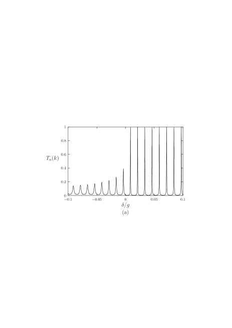
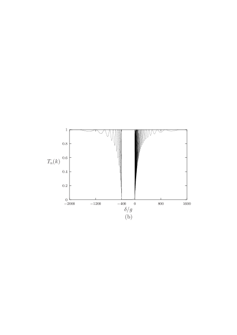
Figure 3: Transmission probability of an excited atom through the mazer with respect to the detuning ($k/\kappa=0.05$, $\kappa L=1000$, $n=0$). The only difference between the two curves resides in the scale used for the horizontal axis.

Same kind of resonances for the transmission probability are observed with respect to the detuning (see fig. 3(a)). For realistic experimental parameters (see discussion in Löffler et al. (1997)), these resonances may even become extremely narrow. Their width amounts only $10^{-2}$ Hz for $\kappa L=10^{5}$, $g=100$ kHz and $k/\kappa=0.01$. This could define very useful metrology devices (atomic clocks for example) based on a single cavity passage and with better performances than what is usually obtained in the well known Ramsey configuration with two cavities or two passages through the same cavity Clairon et al. (1991).

The same curve of the transmission probability is shown on fig. 3(b) over an extended scale. As expected, for very large (positive or negative) detunings, the atom-cavity coupling vanishes and the transmission probability tends towards 1. For large positive detunings, $\theta_{n}\rightarrow\pi/2$ and this behavior is well predicted by Eq. (16) which yields $T_{n}(k)\rightarrow 1$. For large negative detunings, $\theta_{n}\rightarrow 0$ and we get from Eq. (16) $T_{n}(k)\rightarrow 0$. In fact, when increasing the detuning towards negative values, the system leaves the cold atom regime and switches to the hot atom one. For $k\ll\kappa$, this occurs at the detuning value (see Bastin and Martin (2003))

$$-\frac{\delta}{g}=(n+1)\left(\frac{\kappa}{k}\right)^{2}.$$ (25)

For large negative detunings, Eq. (16) is therefore no more valid and the transmission probability must be computed directly using Eqs. (3) and (4). This explains why the transmission probability changes abruptly at $\delta/g~{}\simeq~{}-400$ on fig. 3(b), defining this way a well-defined “window” where the transmission probability drops to a negligible value. This window is all the larger since the atoms are initially colder.

III Velocity selection

If we consider an atomic beam characterized with a velocity distribution $\mathcal{P}_{i}(k)$, each atom will be transmitted through the cavity with more or less efficiency depending on the $T_{n}(k)$ value. The interaction of these atoms with the cavity will lead through the photon emission process to a progressive grow of the cavity photon number. By taking into account the presence of thermal photons and the cavity field damping, Meyer et al. Meyer et al. (1997) have shown that a stationary photon distribution $\mathcal{P}_{\textrm{st}}(n)$ is established inside the cavity. This distribution is given by

$$\mathcal{P}_{\textrm{st}}(n)=\mathcal{P}_{\textrm{st}}(0)\prod_{m=1}^{n}\frac{n_{b}+[r/C]\overline{\mathcal{P}}_{\textrm{em}}(m-1)/m}{n_{b}+1},$$ (26)

where $n_{b}$ is the mean thermal photon number, $r$ is the atomic injection rate, $C$ is the cavity loss rate and $\overline{\mathcal{P}}_{\textrm{em}}(m-1)$ is the mean induced emission probability

$$\overline{\mathcal{P}}_{\textrm{em}}(n)=\int_{0}^{\infty}\mathcal{P}_{\textrm{em}}(n,k)\mathcal{P}_{i}(k)dk,$$ (27)

with $\mathcal{P}_{\textrm{em}}(n,k)$ the induced emission probability of a single atom with momentum $\hbar k$ interacting with the cavity field containing $n$ photons. In presence of a detuning and in the ultracold regime we have shown in Bastin and Martin (2003) that this probability is given by

$$\mathcal{P}_{\textrm{em}}(n,k)=\frac{k_{b}}{k}\frac{\mathcal{I}(L)}{2}\frac{1+\frac{\cot\theta_{n}}{2}\sin(2\kappa_{n}\sqrt{\cot\theta_{n}}L)}{1+\left(\frac{\kappa_{n}}{2k}\right)^{2}\cot\theta_{n}\sin^{2}(\kappa_{n}\sqrt{\cot\theta_{n}}L)}.$$ (28)

After the stationary photon number distribution has been established, the atomic transmission probabilities in the $|a\rangle$ state and the $|b\rangle$ state are respectively given by

$$T^{a}(k)=\sum_{n=0}^{\infty}\mathcal{P}_{\textrm{st}}(n)T^{a}_{n}(k),$$ (29)

and

$$T^{b}(k)=\sum_{n=0}^{\infty}\mathcal{P}_{\textrm{st}}(n)T^{b}_{n+1}(k).$$ (30)

This results in the following final velocity distribution of the transmitted atomic beam :

$$\mathcal{P}_{f}(k)=\left\{\begin{array}[]{ll}P_{i}(k)T^{a}(k)+P_{i}(k^{\prime})T^{b}(k^{\prime})&\textrm{ if }\left(\frac{k}{\kappa}\right)^{2}>-\frac{\delta}{g},\vspace{0.2cm}\\ P_{i}(k)T^{a}(k)&\textrm{ otherwise},\end{array}\right.$$ (31)

where $k^{\prime}$ is such that

$$k^{\prime}_{b}\equiv\sqrt{k^{\prime 2}-\kappa^{2}\frac{\delta}{g}}=k$$ (32)

that is

$$k^{\prime 2}=k^{2}+\kappa^{2}\frac{\delta}{g}$$ (33)

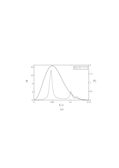
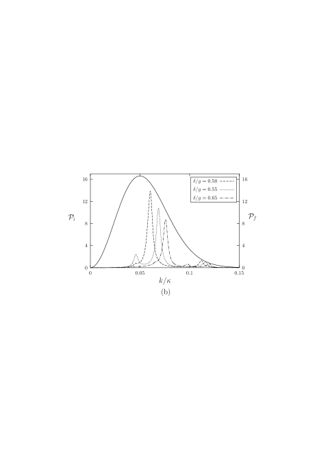
Figure 4: Initial (plain curve) and final (dashed curves) velocity distributions (a) at resonance and (b) for various detuning values. These curves were computed for $\kappa L=200\pi$, $r/C=100$ and $n_{b}=0.2$.

We show on figs. 4 how a Maxwell-Boltzmann distribution (with $k_{0}/\kappa=0.05$ where $k_{0}$ is the most probable wave number) is affected when the atoms are sent through the cavity. The cavity parameters have been taken identical to those considered in Löffler et al. (1998) to underline the detuning effects. We see from these figures that the final distributions are dominated by a narrow single peak whose position depends significantly on the detuning value. This could define a very convenient way to select any desired velocity from an initial broad distribution. Also, notice from the $\mathcal{P}_{f}$ scale that a positive detuning significantly enhances the selection process. Such detunings indeed maximize the resonances of the transmission probability through the cavity (see fig. 3(a)).

IV Summary

In this paper, we have presented the general properties of the transmission probability of ultracold atoms through a micromaser in the general off-resonant case. An analytical expression of this probability has been given in the special case of the mesa mode function. Particularly, we have shown that this probability exhibits with respect to the detuning very fine resonances that could be very useful for metrology devices. We have also demonstrated that the velocity selection in an atomic beam may be significantly enhanced and easily tuned by use of a positive detuning.