Detuning effects in the one-photon mazer

Abstract

The quantum theory of the mazer in the non-resonant case (a detuning between the cavity mode and the atomic transition frequencies is present) is written. The generalization from the resonant case is far from being direct. Interesting effects of the mazer physics are pointed out. In particular, it is shown that the cavity may slow down or speed up the atoms according to the sign of the detuning and that the induced emission process may be completely blocked by use of a positive detuning. It is also shown that the detuning adds a potential step effect not present at resonance and that the use of positive detunings defines a well-controlled cooling mechanism. In the special case of a mesa cavity mode function, generalized expressions for the reflection and transmission coefficients have been obtained. The general properties of the induced emission probability are finally discussed in the hot, intermediate and cold atom regimes. Comparison with the resonant case is given.

I Introduction

The interaction of cold atoms with microwave high-$Q$ cavities (a cold atom micromaser) has recently attracted increasing interest since it was demonstrated by Scully et al. Scully et al. (1996) that this interaction leads to a new type of induced emission inside the cavity. The new emission properties arise from the necessity to treat quantum mechanically the center-of-mass motion of the atoms interacting with the cavity. To insist on the importance of this quantization, usually defined along the $z$ axis, the system was called a mazer (for microwave amplification via $z$-motion-induced emission of radiation). The complete quantum theory of the mazer was described in a series of three papers by Scully and co-workers Meyer et al. (1997); Löffler et al. (1997); Schröder et al. (1997). The theory was written for two-level atoms interacting with a single mode of the high-$Q$ cavity via a one-photon transition. In particular, it was shown that the induced emission properties are strongly dependent on the cavity mode profile. Results were presented for the mesa, sech² and sinusoidal modes. Retamal et al. Retamal et al. (1998) later refined these results in the special case of the sinusoidal mode, and a numerical method was proposed by Bastin and Solano Bastin and Solano (2000) for efficiently computing the mazer properties with arbitrary cavity field modes. Löffler et al. Löffler et al. (1998) showed also that the mazer may be used as a velocity selection device for an atomic beam. The mazer concept was extended by Zhang et al. Zhang et al. (1999a); Zhang and He (1998); Zhang et al. (1999b), who considered two-photon transitions Zhang et al. (1999a), three-level atoms interacting with a single cavity Zhang and He (1998) and with two cavities Zhang et al. (1999b). Collapse and revival patterns with a mazer have been computed by Du et al. Si-de Du et al. (1999). Arun et al. Arun et al. (2000); Arun and Agarwal (2002) studied the mazer with bimodal cavities and Agarwal and Arun Agarwal and Arun (2000) demonstrated resonant tunneling of cold atoms through two mazer cavities.

In all these previous studies, the mazer properties were always presented in the resonant case where the cavity mode frequency $\omega$ is equal to the atomic transition frequency $\omega_{0}$. When three-level atoms were considered, a generalized resonant condition was assumed Zhang and He (1998); Zhang et al. (1999b); Arun et al. (2000). In this paper, we remove this restriction and establish the theory of the mazer in the nonresonant case ($\omega\neq\omega_{0}$) for two-level atoms.

The paper is organized as follows. In Sec. II, the Hamiltonian modeling the mazer in the nonresonant case is presented. The wave functions of the system are described and generalized expressions for the reflection and transmission coefficients in the special case of the mesa mode function are derived. The properties of the induced emission probability when a detuning is present are then discussed in Sec. III. Three regimes of the mazer are considered (hot, intermediate and cold). A brief summary of our results is finally given in Sec. IV.

II Model

II.1 The Hamiltonian

We consider a two-level atom moving along the $z$ direction on the way to a cavity of length $L$. The atom is coupled unresonantly to a single mode of the quantized field present in the cavity. The atomic center-of-mass motion is described quantum mechanically and the usual rotating-wave approximation is made. We thus consider the Hamiltonian

$$H=\hbar\omega_{0}\sigma^{\dagger}\sigma+\hbar\omega a^{\dagger}a+\frac{p^{2}}{2m}+\hbar g\,u(z)(a^{\dagger}\sigma+a\sigma^{\dagger}),$$ (1)

where $p$ is the atomic center-of-mass momentum along the $z$ axis, $m$ is the atomic mass, $\omega_{0}$ is the atomic transition frequency, $\omega$ is the cavity field mode frequency, $\sigma=|b\rangle\langle a|$ ($|a\rangle$ and $|b\rangle$ are, respectively, the upper and lower levels of the two-level atom), $a$ and $a^{\dagger}$ are, respectively, the annihilation and creation operators of the cavity radiation field, $g$ is the atom-field coupling strength, and $u(z)$ is the cavity field mode function. We denote in the following the detuning $\omega-\omega_{0}$ by $\delta$, the cavity field eigenstates by $|n\rangle$ and the global state of the atom-field system by $|\psi(t)\rangle$.

II.2 The wave functions

We introduce the orthonormal basis

$$\begin{array}[]{l}|\Gamma_{n}^{+}(\theta)\rangle=\cos\theta\,|a,n\rangle+\sin\theta\,|b,n+1\rangle,\vspace{8pt}\\ |\Gamma_{n}^{-}(\theta)\rangle=-\sin\theta\,|a,n\rangle+\cos\theta\,|b,n+1\rangle,\end{array}$$ (2)

with $\theta$ an arbitrary parameter. The $|\Gamma_{n}^{\pm}(\theta)\rangle$ states coincide with the noncoupled states $|a,n\rangle$ and $|b,n+1\rangle$ when $\theta=0$ and with the dressed states when $\theta=\theta_{n}$ given by

$$\cot 2\theta_{n}=-\frac{\delta}{\Omega_{n}}\,,$$ (3)

with

$$\Omega_{n}=2g\sqrt{n+1}.$$ (4)

We denote as $|\pm,n\rangle$ the dressed states $|\Gamma_{n}^{\pm}(\theta_{n})\rangle$. The Schrödinger equation reads in the $z$ representation and in the basis (2)

$$i\hbar\frac{\partial}{\partial t}\psi^{+}_{n,\theta}(z,t)=\left[-\frac{\hbar^{2}}{2m}\frac{\partial^{2}}{\partial z^{2}}+(n+1)\hbar\omega-\cos^{2}\theta\>\hbar\delta\;+\;\hbar gu(z)\sqrt{n\!+\!1}\sin 2\theta\right]\psi^{+}_{n,\theta}(z,t)\\ +\bigg{[}\hbar gu(z)\sqrt{n\!+\!1}\;\cos 2\theta+\frac{1}{2}\sin 2\theta\>\hbar\delta\bigg{]}\psi^{-}_{n,\theta}(z,t),$$ (5a)

$$i\hbar\frac{\partial}{\partial t}\psi^{-}_{n,\theta}(z,t)=\left[-\frac{\hbar^{2}}{2m}\frac{\partial^{2}}{\partial z^{2}}+(n+1)\hbar\omega-\sin^{2}\theta\>\hbar\delta\;-\;\hbar gu(z)\sqrt{n\!+\!1}\sin 2\theta\right]\psi^{-}_{n,\theta}(z,t)\\ +\bigg{[}\hbar gu(z)\sqrt{n\!+\!1}\;\cos 2\theta+\frac{1}{2}\sin 2\theta\>\hbar\delta\bigg{]}\psi^{+}_{n,\theta}(z,t),$$ (5b)

with

$$\psi^{\pm}_{n,\theta}(z,t)=\langle z,\Gamma_{n}^{\pm}(\theta)|\psi(t)\rangle.$$ (6)

We get for each $n$ two coupled partial differential equations. In the resonant case ($\delta=0$), these equations may be decoupled over the entire $z$ axis when working in the dressed state basis and the atom-field interaction reduces to an elementary scattering problem over a potential barrier and a potential well defined by the cavity (see Ref. Meyer et al. (1997)). In the presence of detuning, this is no longer the case : there is no basis where Eqs. (5) would separate over the entire $z$ axis and the interpretation of the atomic interaction with the cavity as a scattering problem over two potentials is less evident.

Outside the cavity (which we define to be located in the range $0<z<L$), the mode function $u(z)$ vanishes and Eqs. (5) become in the noncoupled state basis ($\theta=0$)

$$i\hbar\frac{\partial}{\partial t}\psi^{a}_{n}(z,t) = \left[-\frac{\hbar^{2}}{2m}\frac{\partial^{2}}{\partial z^{2}}\right]\psi^{a}_{n}(z,t),$$ (7a)

$$i\hbar\frac{\partial}{\partial t}\psi^{b}_{n+1}(z,t) = \left[-\frac{\hbar^{2}}{2m}\frac{\partial^{2}}{\partial z^{2}}+\hbar\delta\right]\psi^{b}_{n+1}(z,t),$$ (7b)

with

$$\psi^{a}_{n}(z,t) = e^{i(\omega_{0}+n\omega)t}\langle z,a,n|\psi(t)\rangle,\phantom{\bigg{|}}$$ (8a)

$$\psi^{b}_{n+1}(z,t) = e^{i(\omega_{0}+n\omega)t}\langle z,b,n+1|\psi(t)\rangle.$$ (8b)

In Eqs. (8), we have introduced the exponential factor $e^{i(\omega_{0}+n\omega)t}$ in order to define the energy scale origin at the $|a,n\rangle$ level. The solutions to Eqs. (7) are obviously given by linear combinations of plane wave functions. If we assume initially a monokinetic atom (with momentum $\hbar k$) coming upon the cavity from the left side (negative $z$ values) in the excited state $|a\rangle$ and the cavity field in the number state $|n\rangle$, the atom-field system is described outside the cavity by the wave function components (which correspond to the eigenstate $|\phi_{k}\rangle$ of energy $E_{k}=\hbar^{2}k^{2}/2m$)

$$\psi^{a}_{n}(z,t) = e^{-i\frac{\hbar k^{2}}{2m}t}\varphi^{a}_{n}(z),\phantom{\bigg{|}}$$ (9a)

$$\psi^{b}_{n+1}(z,t) = e^{-i\frac{\hbar k^{2}}{2m}t}\varphi^{b}_{n+1}(z),$$ (9b)

with

$$\varphi^{a}_{n}(z)\;\,=\;\,\left\{\begin{array}[]{ll}e^{ikz}+\rho^{a}_{n}\,e^{-ikz}&\;z<0,\vspace{0.2cm}\\ \tau^{a}_{n}\,e^{ik(z-L)}&\;z>L,\end{array}\right.$$ (12)

$$\varphi^{b}_{n+1}(z)=\left\{\begin{array}[]{ll}\rho^{b}_{n+1}\,e^{-ik_{b}z}&\;\;z<0,\vspace{0.2cm}\\ \tau^{b}_{n+1}\,e^{ik_{b}(z-L)}&\;\;z>L,\end{array}\right.$$ (15)

and

$$k^{2}_{b}=k^{2}-\frac{2m\delta}{\hbar}.$$ (16)

Introducing

$$\kappa^{2}=\frac{2mg}{\hbar}$$ (17)

we may write

$$k^{2}_{b}=k^{2}-\kappa^{2}\frac{\delta}{g}.$$ (18)

The solutions (9) must be interpreted as follows : the excited atom coming upon the cavity will be found reflected in the upper state or in the lower state with the amplitude $\rho^{a}_{n}$ and $\rho^{b}_{n+1}$, respectively, or transmitted with the amplitude $\tau^{a}_{n}$ or $\tau^{b}_{n+1}$. However, in contrast to the resonant case, the atom reflected or transmitted in the lower state $|b\rangle$ will be found to propagate with a momentum $\hbar k_{b}$ different from its initial value $\hbar k$. The atomic transition $|a\rangle\rightarrow|b\rangle$ induced by the cavity is responsible for a change of the atomic kinetic energy. According to the sign of the detuning [see Eq. (18)], the cavity will either speed up the atom (for $\delta<0$) or slow it down (for $\delta>0$). This results merely from energy conservation. When, after leaving the cavity region, the atom is passed from the excited state $|a\rangle$ to the lower state $|b\rangle$, the photon number has increased by one unit in the cavity and the internal energy of the atom-field system has varied by the quantity $\hbar\omega-\hbar\omega_{0}=\hbar\delta$. This variation needs to be exactly counterbalanced by the external energy of the system, i.e., the atomic kinetic energy. In this sense, when a photon is emitted inside the cavity by the atom, the cavity acts as a potential step $\hbar\delta$ (see Fig. 1), and the atom experiences an attractive or a repulsive force according to the sign of the detuning. Similar (although not identical) mechanical effects are obtained under the adiabatic approximation Haroche et al. (1991) (requiring no quantum treatment of the atomic center-of-mass motion). In this case, the dressed levels may also decelerate or accelerate the atoms. However, in this regime and contrary to what is described here, the atom always leaves the cavity with the same kinetic energy (if no dissipation process is considered) and the mechanical effects are not related to the emission of a photon inside the cavity.

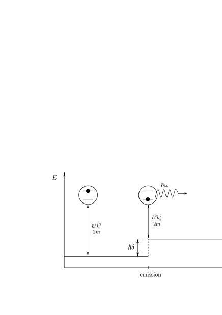
Figure 1: Potential step effect of the cavity when a photon is emitted by the atom. $E$ represents the total energy of the atom-field system.

Presently the use of positive detunings in the atom-field interaction defines a well-controlled cooling mechanism. A single excitation exchange between the atom and the field inside the cavity is sufficient to cool the atom to a desired temperature $T=\hbar^{2}k_{b}^{2}/2mk_{B}$ ($k_{B}$ is the Boltzmann constant) which may in principle be as low as imaginable. However, if the initial atomic kinetic energy $\hbar^{2}k^{2}/2m$ is lower than $\hbar\delta$ (i.e., if $k/\kappa<\sqrt{\delta/g}$), the transition $|a,n\rangle\rightarrow|b,n+1\rangle$ cannot take place (as it would remove $\hbar\delta$ from the kinetic energy) and no photon can be emitted inside the cavity. In this case the emission process is completely blocked.

Due to this change in the kinetic energy when a photon is emitted, the reflection and transmission probabilities of the atom in the lower state $|b\rangle$ are given, respectively, by (for $\hbar^{2}k^{2}/2m>\hbar\delta$)

$$R^{b}_{n+1} =\frac{k_{b}}{k}|\rho^{b}_{n+1}|^{2},$$ (19a)

$$T^{b}_{n+1} =\frac{k_{b}}{k}|\tau^{b}_{n+1}|^{2}.$$ (19b)

These probabilities vanish for $\hbar^{2}k^{2}/2m\leq\hbar\delta$. When the atom remains in the excited state $|a\rangle$ after having interacted with the cavity, there is no change in the atomic kinetic energy and the reflection and transmission probabilities are directly given by

$$R^{a}_{n} =|\rho^{a}_{n}|^{2},$$ (20a)

$$T^{a}_{n} =|\tau^{a}_{n}|^{2}.$$ (20b)

To calculate any quantity related to the reflection and transmission coefficients, we must solve the Schrödinger equation over the entire $z$ axis. Inside the cavity, the problem is much more complex since we have two coupled partial differential equations. In the special case of the mesa mode function [$u(z)=1$ inside the cavity, 0 elsewhere], the problem is, however, greatly simplified. In the dressed state basis ($\theta=\theta_{n}$), the Schrödinger equations (5) take the following form inside the cavity :

$$i\hbar\frac{\partial}{\partial t}\psi^{\pm}_{n}(z,t)=\left[-\frac{\hbar^{2}}{2m}\frac{\partial^{2}}{\partial z^{2}}+V^{\pm}_{n}\right]\psi^{\pm}_{n}(z,t)$$ (21)

with

$$\psi^{\pm}_{n}(z,t)=e^{i(\omega_{0}+n\omega)t}\langle z,\pm,n|\psi(t)\rangle$$ (22)

and

$$V^{+}_{n} =\sin^{2}\theta_{n}\,\hbar\delta+\hbar g\sqrt{n+1}\,\sin 2\theta_{n},\phantom{\bigg{|}}$$ (23a)

$$V^{-}_{n} =\hbar\delta-V^{+}_{n}.$$ (23b)

$V^{+}_{n}$ and $V^{-}_{n}$ represent the internal energies of the $|+,n\rangle$ and $|-,n\rangle$ components, respectively. Except for the resonant case, they cannot be strictly interpreted as a potential barrier and a potential well as Eq. (21) holds only inside the cavity.

Using Eq. (3), we have the well-known relations

$$\begin{array}[]{l}\sin\theta_{n}=\frac{\sqrt{\Lambda_{n}+\delta}}{\sqrt{2\Lambda_{n}}},\vspace{0.3cm}\\ \cos\theta_{n}=\frac{\sqrt{\Lambda_{n}-\delta}}{\sqrt{2\Lambda_{n}}},\end{array}\quad\begin{array}[]{l}\tan\theta_{n}=\sqrt{\frac{\Lambda_{n}+\delta}{\Lambda_{n}-\delta}},\vspace{0.3cm}\\ \cot\theta_{n}=\sqrt{\frac{\Lambda_{n}-\delta}{\Lambda_{n}+\delta}},\end{array}$$ (24)

with

$$\Lambda_{n}=\sqrt{\delta^{2}+\Omega_{n}^{2}}.$$ (25)

We thus have

$$V^{+}_{n} =\hbar g\sqrt{n+1}\tan\theta_{n},\phantom{\bigg{|}}$$ (26a)

$$V^{-}_{n} =-\hbar g\sqrt{n+1}\cot\theta_{n}.$$ (26b)

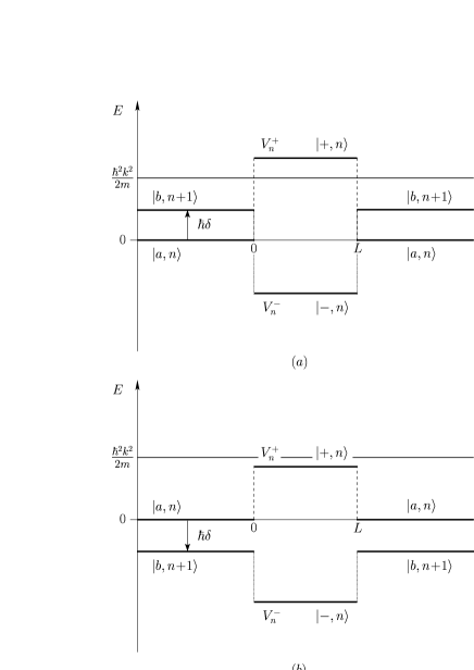
Figure 2: Schematic energy diagram of the atom-field system inside and outside the cavity, for $\delta>0$ (a) and $\delta<0$ (b).

The exponential factor $e^{i(\omega_{0}+n\omega)t}$ has been introduced as well in Eq. (22) in order to define the same energy scale inside and outside the cavity. Figure 2 illustrates the internal energies of the atom-field system over the whole $z$ axis. The positive internal energy $V^{+}_{n}$ increases with positive detunings and vice versa with negative ones. For a fixed value of the incident kinetic energy $E_{k}=\hbar^{2}k^{2}/2m$, $V^{+}_{n}$ may be switched in this way from a higher value than $E_{k}$ to a lower one. For large positive (negative) detunings, $V^{+}_{n}$ tends to the $|b,n+1\rangle$ ($|a,n\rangle$) state energy.

The most general solution of Eqs. (21) corresponding to the eigenstate $|\phi_{k}\rangle$ is given by

$$\psi^{\pm}_{n}(z,t)=e^{-i\frac{\hbar k^{2}}{2m}t}\varphi^{\pm}_{n}(z)$$ (27)

with

$$\varphi^{\pm}_{n}(z)=A^{\pm}_{n}e^{ik^{\pm}_{n}z}+B^{\pm}_{n}e^{-ik^{\pm}_{n}z},$$ (28)

where $A^{\pm}_{n}$ and $B^{\pm}_{n}$ are complex coefficients and

$${k^{\pm}_{n}}^{2}=k^{2}-\frac{2m}{\hbar^{2}}V^{\pm}_{n}.$$ (29)

Defining

$$\kappa_{n}=\kappa\sqrt[4]{n+1},$$ (30)

we have

$${k^{+}_{n}}^{2} =k^{2}-\kappa_{n}^{2}\tan\theta_{n},\phantom{\bigg{|}}$$ (31a)

$${k^{-}_{n}}^{2} =k^{2}+\kappa_{n}^{2}\cot\theta_{n}.$$ (31b)

Using Eq. (23b), we may also write

$${k^{-}_{n}}^{2}=k_{b}^{2}+\kappa_{n}^{2}\tan\theta_{n}.$$ (32)

From Eq. (2), we may express the wave function components of the atom-field state inside the cavity over the noncoupled state basis. We have

$$\psi^{a}_{n}(z,t) =\cos\theta_{n}\psi^{+}_{n}(z,t)-\sin\theta_{n}\psi^{-}_{n}(z,t),\phantom{\bigg{|}}$$ (33a)

$$\psi^{b}_{n+1}(z,t) =\sin\theta_{n}\psi^{+}_{n}(z,t)+\cos\theta_{n}\psi^{-}_{n}(z,t).$$ (33b)

This allows us to find the wave function components of the eigenstate $|\phi_{k}\rangle$ over the entire $z$ axis. The relations (9) hold with

$$\varphi^{a}_{n}(z)\;\,=\;\,\left\{\begin{array}[]{ll}e^{ikz}+\rho^{a}_{n}\,e^{-ikz}&\;z<0,\vspace{0.2cm}\\ \varphi^{a}_{n}(z)\big{|}_{C}&\;0<z<L,\vspace{0.2cm}\\ \tau^{a}_{n}\,e^{ik(z-L)}&\;z>L,\end{array}\right.$$ (37)

$$\varphi^{b}_{n+1}(z)=\left\{\begin{array}[]{ll}\rho^{b}_{n+1}\,e^{-ik_{b}z}&\;\;z<0,\vspace{0.2cm}\\ \varphi^{b}_{n+1}(z)\big{|}_{C}&\;\;0<z<L,\vspace{0.2cm}\\ \tau^{b}_{n+1}\,e^{ik_{b}(z-L)}&\;\;z>L,\end{array}\right.$$ (41)

and

$$\varphi^{a}_{n}(z)\big{|}_{C} =\cos\theta_{n}\left(A^{+}_{n}e^{ik^{+}_{n}z}+B^{+}_{n}e^{-ik^{+}_{n}z}\right)$$

$$\quad-\sin\theta_{n}\left(A^{-}_{n}e^{ik^{-}_{n}z}+B^{-}_{n}e^{-ik^{-}_{n}z}\right),\phantom{\bigg{|}}$$ (42a)

$$\varphi^{b}_{n+1}(z)\big{|}_{C} =\sin\theta_{n}\left(A^{+}_{n}e^{ik^{+}_{n}z}+B^{+}_{n}e^{-ik^{+}_{n}z}\right)$$

$$\quad+\cos\theta_{n}\left(A^{-}_{n}e^{ik^{-}_{n}z}+B^{-}_{n}e^{-ik^{-}_{n}z}\right).$$ (42b)

The coefficients $\rho^{a}_{n}$, $\rho^{b}_{n+1}$, $\tau^{a}_{n}$, $\tau^{b}_{n+1}$, $A^{+}_{n}$, $A^{-}_{n}$, $B^{+}_{n}$, and $B^{-}_{n}$ in expressions (37)-(42) are found by imposing the continuity conditions on the wave function and its first derivative at the cavity interfaces. A tedious calculation yields

$$\tau^{a}_{n} =\frac{\cos^{2}\theta_{n}\frac{\tau^{-}_{n}(k)}{\tau^{-}_{n}(k_{b})}\,\tau^{+}_{n}(k_{b})+\sin^{2}\theta_{n}\,{\tau^{-}_{n}(k)}}{\left(\cos^{2}\theta_{n}\frac{k-k_{b}}{k^{c}_{n}(L)}-1\right)\left(\cos^{2}\theta_{n}\frac{k-k_{b}}{k^{t}_{n}(L)}-1\right)},$$ (43)

$$\rho^{a}_{n} =\frac{\cos^{2}\theta_{n}\frac{\tau^{-}_{n}(k)}{\tau^{\prime-}_{n}(k,k_{b})}\frac{\Delta^{+}_{n}(k)}{\Delta^{+}_{n}(k_{b})}\rho^{+}_{n}(k_{b})+\left(1-\cos^{2}\theta_{n}\frac{\tau^{+}_{n}(k_{b})}{\tau^{\prime\prime+}_{n}(k,k_{b})}\right)\rho^{-}_{n}(k)+\frac{\cos^{2}\theta_{n}}{4}\left(\frac{k_{b}}{k}-\frac{k}{k_{b}}\right)u_{n}(k)\frac{\rho^{-}_{n}(k)\rho^{+}_{n}(k_{b})}{\Delta^{-}_{n}(k)\Delta^{+}_{n}(k_{b})}}{\left(\cos^{2}\theta_{n}\frac{k-k_{b}}{k^{c}_{n}(L)}-1\right)\left(\cos^{2}\theta_{n}\frac{k-k_{b}}{k^{t}_{n}(L)}-1\right)},$$ (44)

$$\tau^{b}_{n+1} =\frac{\sin 2\theta_{n}}{4}\left(1+\frac{k}{k_{b}}\right)\frac{\frac{\tau^{-}_{n}(k)}{\tilde{\tau}^{-}_{n}(k,k_{b})}\,\tau^{+}_{n}(k_{b})-\frac{\tau^{+}_{n}(k_{b})}{\tilde{\tau}^{+}_{n}(k,k_{b})}\,\tau^{-}_{n}(k)}{\left(\cos^{2}\theta_{n}\frac{k-k_{b}}{k^{c}_{n}(L)}-1\right)\left(\cos^{2}\theta_{n}\frac{k-k_{b}}{k^{t}_{n}(L)}-1\right)},$$ (45)

$$\rho^{b}_{n+1} =\sin 2\theta_{n}\frac{\frac{1}{2}\frac{\tau^{-}_{n}(k)}{\bar{\tau}^{-}_{n}(k,k_{b})}\frac{\Delta^{+}_{n}(k)}{\Delta^{+}_{n}(k_{b})}\rho^{+}_{n}(k_{b})-\frac{1}{2}\frac{\tau^{+}_{n}(k_{b})}{\bar{\tau}^{+}_{n}(k,k_{b})}\rho^{-}_{n}(k)+\frac{1}{4}\left(\frac{k}{k_{b}}-1\right)v_{n}(k)\tau^{-}_{n}(k)\tau^{+}_{n}(k_{b})}{\left(\cos^{2}\theta_{n}\frac{k-k_{b}}{k^{c}_{n}(L)}-1\right)\left(\cos^{2}\theta_{n}\frac{k-k_{b}}{k^{t}_{n}(L)}-1\right)},$$ (46)

with

$$u_{n}(k) =\sin^{2}\theta_{n}\frac{S^{+-}_{n}}{\sin(k^{+}_{n}L)\sin(k^{-}_{n}L)}+\left(\frac{k^{-}_{n}k^{+}_{n}}{k^{2}}-\frac{k^{2}}{k^{-}_{n}k^{+}_{n}}\right),$$ (47)

$$v_{n}(k) =i\left(\frac{k^{+}_{n}}{k}\sin(k^{+}_{n}L)\cos(k^{-}_{n}L)-\frac{k^{-}_{n}}{k}\sin(k^{-}_{n}L)\cos(k^{+}_{n}L)\right)-\frac{\cos 2\theta_{n}}{2}S^{+-}_{n},$$ (48)

$$S^{+-}_{n} =\sin(k^{+}_{n}L)\sin(k^{-}_{n}L)\left(\frac{k^{-}_{n}}{k^{+}_{n}}+\frac{k^{+}_{n}}{k^{-}_{n}}\right)+2(\cos(k^{-}_{n}L)\cos(k^{+}_{n}L)-1),$$ (49)

and

$$\rho^{\pm}_{n}(k)=i\Delta^{\pm}_{n}(k)\sin(k^{\pm}_{n}L)\tau^{\pm}_{n}(k),$$ (50)

$$\tau^{\pm}_{n}(k)=\left[\cos(k^{\pm}_{n}L)-i\Sigma^{\pm}_{n}(k)\sin(k^{\pm}_{n}L)\right]^{-1},$$ (51)

$$\Sigma^{\pm}_{n}(k)=\frac{1}{2}\left(\frac{k^{\pm}_{n}}{k}+\frac{k}{k^{\pm}_{n}}\right),$$ (52)

$$\Delta^{\pm}_{n}(k)=\frac{1}{2}\left(\frac{k^{\pm}_{n}}{k}-\frac{k}{k^{\pm}_{n}}\right),$$ (53)

$$\tau^{\prime\pm}_{n}(k,k_{b})=\left[\cos(k^{\pm}_{n}L)-i\frac{k_{b}}{k}\Sigma^{\pm}_{n}(k)\sin(k^{\pm}_{n}L)\right]^{-1}\!\!\!\!,$$ (54)

$$\tau^{\prime\prime\pm}_{n}(k,k_{b})=\left[\cos(k^{\pm}_{n}L)-i\frac{k}{k_{b}}\Sigma^{\pm}_{n}(k)\sin(k^{\pm}_{n}L)\right]^{-1}\!\!\!\!,$$ (55)

$$\tilde{\tau}^{\pm}_{n}(k,k_{b})=\left[\cos(k^{\pm}_{n}L)-i\tilde{\Sigma}^{\pm}_{n}(k,k_{b})\sin(k^{\pm}_{n}L)\right]^{-1},$$ (56)

$$\bar{\tau}^{\pm}_{n}(k,k_{b})=\left[\cos(k^{\pm}_{n}L)-i\frac{k+k_{b}}{2k_{b}}\Sigma^{\pm}_{n}(k)\sin(k^{\pm}_{n}L)\right]^{-1}\!\!\!\!,$$ (57)

$$\tilde{\Sigma}^{\pm}_{n}(k,k_{b})=\left(\frac{k^{\pm}_{n}}{k+k_{b}}+\frac{k_{b}}{k+k_{b}}\frac{k}{k^{\pm}_{n}}\right),$$ (58)

$$k^{c}_{n}(L)=i\frac{\left(k+i\cot(\frac{k^{-}_{n}L}{2})k^{-}_{n}\right)\left(k_{b}+i\cot(\frac{k^{+}_{n}L}{2})k^{+}_{n}\right)}{\cot(\frac{k^{-}_{n}L}{2})k^{-}_{n}-\cot(\frac{k^{+}_{n}L}{2})k^{+}_{n}},$$ (59)

$$k^{t}_{n}(L)=i\frac{\left(k-i\tan(\frac{k^{-}_{n}L}{2})k^{-}_{n}\right)\left(k_{b}-i\tan(\frac{k^{+}_{n}L}{2})k^{+}_{n}\right)}{\tan(\frac{k^{+}_{n}L}{2})k^{+}_{n}-\tan(\frac{k^{-}_{n}L}{2})k^{-}_{n}}.$$ (60)

At resonance, $\delta=0$, $\theta_{n}=\pi/4$, $k_{b}=k$, $\tau^{\pm}_{n}(k)=\tau^{\prime\pm}_{n}(k,k_{b})=\tau^{\prime\prime\pm}_{n}(k,k_{b})=\tilde{\tau}^{\pm}_{n}(k,k_{b})=\bar{\tau}^{\pm}_{n}(k,k_{b})$ and the reflection and transmission coefficients reduce to the well-known results (see Ref. Meyer et al. (1997))

$$\tau^{a}_{n}=\frac{1}{2}\left(\tau^{+}_{n}+\tau^{-}_{n}\right),$$ (61a)

$$\rho^{a}_{n}=\frac{1}{2}\left(\rho^{+}_{n}+\rho^{-}_{n}\right),$$ (61b)

and

$$\tau^{b}_{n+1}=\frac{1}{2}\left(\tau^{+}_{n}-\tau^{-}_{n}\right),$$ (62a)

$$\rho^{b}_{n+1}=\frac{1}{2}\left(\rho^{+}_{n}-\rho^{-}_{n}\right).$$ (62b)

III Induced emission probability

The induced emission probability of a photon inside the cavity is given by

$$\mathcal{P}_{\textrm{em}}(n)=R^{b}_{n+1}+T^{b}_{n+1}.$$ (63)

According to Eqs. (19), this probability may be written as

$$\mathcal{P}_{\textrm{em}}(n)=\left\{\begin{array}[]{ll}\frac{k_{b}}{k}\Big{(}\,|\rho^{b}_{n+1}|^{2}+|\tau^{b}_{n+1}|^{2}\,\Big{)}&\text{if }\frac{k}{\kappa}>\sqrt{\frac{\delta}{g}},\vspace{0.2cm}\\ 0&\text{otherwise.}\end{array}\right.$$ (64)

We distinguish three regimes determined by the incident kinetic energy of the atom compared with the internal energy $V_{n}^{+}$ (see Fig. 2) : the hot atom regime (when $k\gg\kappa_{n}\sqrt{\tan\theta_{n}}$ and $k_{b}$ is approximated to $k$), the intermediate regime ($k\approx\kappa_{n}\sqrt{\tan\theta_{n}}$) and the cold atom regime ($k\ll\kappa_{n}\sqrt{\tan\theta_{n}}$). In comparison with the resonant case, the detuning defines an additional parameter that fixes the working regime of the system.

III.1 Hot atom regime

In the hot atom regime, the kinetic energy is much higher than the energies $V_{n}^{\pm}$ and the atoms are always transmitted through the cavity. For the mesa mode, the atomic momentum inside the cavity is given by

$$\hbar k_{n}^{+}\simeq\hbar k\left(1-\frac{\kappa_{n}^{2}}{2k^{2}}\tan\theta_{n}\right),$$ (65a)

$$\hbar k_{n}^{-}\simeq\hbar k\left(1+\frac{\kappa_{n}^{2}}{2k^{2}}\cot\theta_{n}\right).$$ (65b)

After the atom-field interaction, the global state of the system reduces to

$$\begin{split}|\psi(t)\rangle=\int\!dz\,\psi(z,t)&\left(\cos\theta_{n}e^{-i\frac{\kappa_{n}^{2}L}{2k}\tan\theta_{n}}|z,+,n\rangle\right.\\ &\left.-\sin\theta_{n}e^{i\frac{\kappa_{n}^{2}L}{2k}\cot\theta_{n}}|z,-,n\rangle\right)\end{split}$$ (66)

with

$$\psi(z,t)=e^{ikz}e^{-i\frac{\hbar k^{2}}{2m}t}.$$ (67)

The induced emission probability is thus given by

$$\begin{split}\mathcal{P}_{\textrm{em}}(n)&=|\langle z,b,n+1|\psi(t)\rangle|^{2}\\ &=\frac{\sin^{2}(2\theta_{n})}{4}\left|\,e^{-i\frac{\kappa_{n}^{2}L}{2k}\tan\theta_{n}}-e^{i\frac{\kappa_{n}^{2}L}{2k}\cot\theta_{n}}\right|^{2}.\end{split}$$ (68)

Using Eq. (24) we get straightforwardly

$$\mathcal{P}_{\textrm{em}}(n)=\left[1+\left(\frac{\delta}{\Omega_{n}}\right)^{2}\right]^{-1}\sin^{2}\left(\frac{\tau}{2}\sqrt{\Omega_{n}^{2}+\delta^{2}}\right),$$ (69)

where $\tau=\frac{mL}{\hbar k}$ is the classical transit time of the thermal atoms through the cavity.

Equation (69) is exactly the classical expression of the induced emission probability of an atom interacting with a single mode during a time $\tau$. We recover the well-known Rabi oscillations in the general case where the field and the atomic frequencies are detuned by the quantity $\delta$.

III.2 Intermediate regime

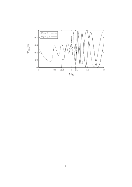
Figure 3: Induced emission probability $\mathcal{P}_{\textrm{em}}(n=0)$ with respect to $k/\kappa$ (for $\kappa L=10\pi$ and two different values of the detuning).

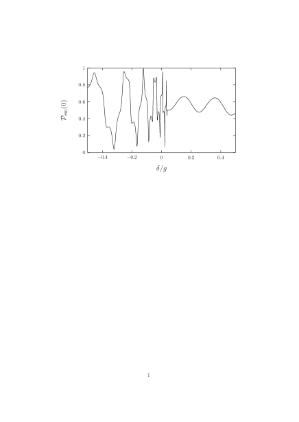
Figure 4: Induced emission probability $\mathcal{P}_{\textrm{em}}(n=0)$ with respect to $\delta/g$ in the intermediate regime ($k/\kappa=1.01$). The interaction length was fixed to $\kappa L=100$.

The frontier between the cold atom and the hot atom regime appears when the atomic kinetic energy becomes equal to the positive energy $V^{+}_{n}$ inside the cavity, i.e., when the ratio $k/\kappa_{n}$ is equal to the critical value

$$\left.\frac{k}{\kappa_{n}}\right|_{c}=\sqrt{\tan\theta_{n}}=\left(\frac{\sqrt{\left(\frac{\delta}{g}\right)^{2}+4(n+1)}\,+\,\frac{\delta}{g}}{\sqrt{\left(\frac{\delta}{g}\right)^{2}+4(n+1)}\,-\,\frac{\delta}{g}}\right)^{\frac{1}{4}}$$ (70)

At resonance, this frontier occurs for $k/\kappa_{n}=1$. This condition changes significantly when the cavity and the atomic transition are detuned. This is well illustrated in Fig. 3, which shows the induced emission probability as a function of $k/\kappa$ at resonance and for a positive value of the detuning. In the second case, the regime change occurs for a larger value of $k/\kappa$ than one. Please notice also that the induced emission probability vanishes for $k/\kappa<\sqrt{\delta/g}$ according to Eq. (64).

Equation (70) may be inverted to yield a critical detuning when working with a fixed value of $k/\kappa$. We get

$$\left.\frac{\delta}{g}\right|_{c}=\sqrt{n+1}\left[\left(\frac{k}{\kappa_{n}}\right)^{2}-\left(\frac{k}{\kappa_{n}}\right)^{\!\!-2}\right].$$ (71)

Figure 4 illustrates the induced emission probability as a function of the detuning for $k/\kappa$ slightly greater than one. At resonance, the system is on the hot atom regime side as the atomic kinetic energy is greater than the internal energy $V^{+}_{n}$. When the detuning is increased, $V^{+}_{n}$ is increased as well and becomes greater than the kinetic energy [see Fig. 2(a)], switching the system toward the cold atom regime. This therefore could define a convenient way to switch from one regime to the other rather than varying the incident atomic momentum.

A similar effect of the detuning is presented in Fig. 5 which presents the induced emission probability with respect to the interaction length in the intermediate regime. It appears clearly there that working with a negative detuning is similar to working with hotter atoms at resonance. This results merely from the level of $V^{+}_{n}$ compared to the incident kinetic energy, which is identical in both cases considered in Fig. 5.

From all these situations, we conclude that a detuning variation has an identical effect than a change of the kinetic energy of the incoming atoms, confirming that the only important parameter of the system in the intermediate regime is the actual value of the $V^{+}_{n}$ energy in comparison with the kinetic energy $\hbar^{2}k^{2}/2m$.

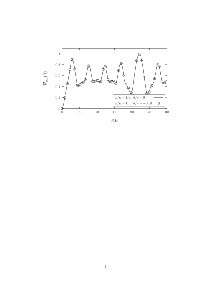
Figure 5: Induced emission probability $\mathcal{P}_{\textrm{em}}(n=0)$ with respect to the interaction length $\kappa L$ in the intermediate regime. Comparison of a detuning variation with a change of the atomic kinetic energy.

III.3 Cold atom regime

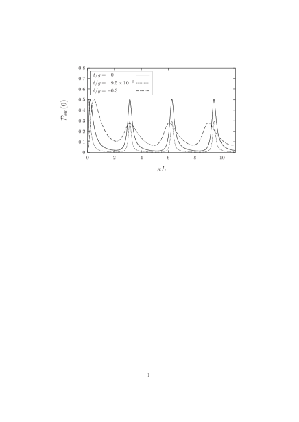
Figure 6: Induced emission probability $\mathcal{P}_{\textrm{em}}(n=0)$ with respect to the interaction length $\kappa L$ in the cold atom regime ($k/\kappa=0.1$) and for various values of the detuning.

In the cold atom regime ($k/\kappa_{n}\ll\sqrt{\tan\theta_{n}}$), the induced emission probability exhibits a completely different behavior. We have in this regime for $|\delta|/\Omega_{n}\ll 1$, $\exp(\kappa_{n}L)\gg 1$, and $\kappa_{n}L\ll(\kappa_{n}/k)^{2}$,

$$\mathcal{P}_{\textrm{em}}(n)=\frac{\mathcal{B}(L)}{2}\frac{1+\frac{\cot\theta_{n}}{2}\sin(2\kappa_{n}\sqrt{\cot\theta_{n}}L)}{1+\left(\frac{\kappa_{n}}{2k}\right)^{2}\cot\theta_{n}\sin^{2}(\kappa_{n}\sqrt{\cot\theta_{n}}L)},$$ (72)

with

$$\mathcal{B}(L)=\frac{k_{b}}{k}\frac{1}{\left|\cos^{2}\theta_{n}\frac{k-k_{b}}{k^{c}_{n}(L)}-1\right|^{2}\left|\cos^{2}\theta_{n}\frac{k-k_{b}}{k^{t}_{n}(L)}-1\right|^{2}}.$$ (73)

At resonance, this expression simplifies to

$$\mathcal{P}_{\textrm{em}}(n)=\frac{1}{2}\frac{1+\frac{1}{2}\sin(2\kappa_{n}L)}{1+\left(\frac{\kappa_{n}}{2k}\right)^{2}\sin^{2}(\kappa_{n}L)}$$ (74)

and the results of Meyer et al. Meyer et al. (1997) are well recovered. Figure 6 illustrates the induced emission probability (72) with respect to the interaction length $\kappa L$ for various values of the detuning. The curves present a series of peaks where the induced emission probability is optimum. The detuning affects the peak position, amplitude, and width. Similarly to the resonant case, the curves still look like the Airy function of classical optics $[1+F\sin^{2}(\Delta/2)]^{-1}$ with finesse $F$ and total phase difference $\Delta$, even if the structure of Eq. (72) has become complicated with the factor $\mathcal{B}(L)$. In fact, this equation is extremely well fitted in its domain of validity by the function

$$\mathcal{P}_{\textrm{em}}(n)=\frac{2k_{b}/k}{(1+k_{b}/k)^{2}}\frac{1+\frac{1}{2}\sin(2\kappa_{n}\sqrt{\cot\theta_{n}}L)}{1+(\frac{\kappa_{n}}{k_{b}+k})^{2}\sin^{2}(\kappa_{n}\sqrt{\cot\theta_{n}}L)}.$$ (75)

III.3.1 Peak position

The induced emission probability is optimum when

$$\kappa_{n}\sqrt{\cot\theta_{n}}L=m\pi\quad(m\textrm{ a positive integer}).$$ (76)

This occurs when the cavity length fits a multiple of one-half the de Broglie wavelength $\lambda_{\mathrm{dB}}$ of the atom inside the cavity :

$$L=m\frac{\lambda_{\mathrm{dB}}}{2}.$$ (77)

Indeed, in the cold atom regime, only the $|-,n\rangle$ component propagates inside the cavity with the de Broglie wavelength

$$\lambda_{\mathrm{dB}}=\frac{2\pi}{k^{-}_{n}}\simeq\frac{2\pi}{\kappa_{n}\sqrt{\cot\theta_{n}}}.$$ (78)

Inserting Eq. (78) into Eq. (77) gives the condition (76).

III.3.2 Peak amplitude

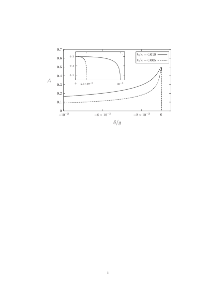
Figure 7: Amplitude $\mathcal{A}$ of the resonances with respect to $\delta/g$ for two values of $k/\kappa$ in the cold atom regime.

The peak amplitude of the induced emission probability $\mathcal{P}_{\textrm{em}}(n)$ is given by

$$\mathcal{A}\equiv\frac{\mathcal{B}(L=m\frac{\lambda_{\mathrm{dB}}}{2})}{2}\simeq\frac{1}{2}\frac{4k_{b}/k}{(1+k_{b}/k)^{2}}.$$ (79)

We illustrate this amplitude in Fig. 7 as a function of the detuning $\delta$. In contrast to the hot atom regime [see Eq. (69)], the curves present a strong asymmetry with respect to the sign of the detuning. This results from the potential step $\hbar\delta$ (see Sec. II.) experienced by the atoms when they emit a photon. For cold atoms whose energy is similar or less than the step height, the sign of the step is a crucial parameter. According to Eq. (64), the induced emission probability drops down very rapidly to zero for positive detunings, in contrast to what happens for negative detunings.

It is also interesting to note that the peak amplitude (79) is equal to the amplitude at resonance ($1/2$) times the factor $(4k_{b}/k)/(1+k_{b}/k)^{2}$ that corresponds exactly to the transmission factor of a particle of momentum $\hbar k$ through a potential step $\hbar\delta$. This is an additional argument to say that the use of a detuning adds a potential step effect for the atoms emitting a photon inside the cavity (see Fig. 1).

III.3.3 Peak width

The peak width is determined by the finesse $(\frac{\kappa_{n}}{k_{b}+k})^{2}$. Positive detunings increase the finesse ($k_{b}<k$) while negative ones decrease it ($k_{b}>k$).

III.3.4 Large detunings

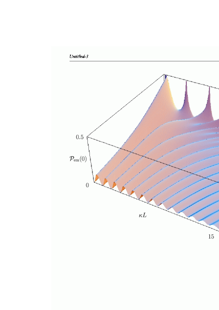
Figure 8: Induced emission probability $\mathcal{P}_{\textrm{em}}(n=0)$ with respect to the interaction length $\kappa L$ and $\delta/g$ (for $k/\kappa=0.1$).

For large detunings, Eq. (72) is no longer valid and the induced emission probability must be computed using the general relation (64). We present in Fig. 8 $\mathcal{P}_{\textrm{em}}(0)$ as a function of the detuning and the interaction length $\kappa L$. The variation of the resonance positions with respect to the detuning is very clear in this figure. It is interesting to note that one resonance out of two disappears when increasing the detuning toward negative values. Also, the induced emission probability does not decrease monotonically with the detuning (especially for small interaction lengths). This effect is strictly limited to the cold atom regime as for hot atoms the Rabi oscillation amplitudes always decrease when larger and larger detunings are used [see Eq. (69)].

The use of large negative detunings in the cold atom regime is not limitless. As $-\delta$ increases, the internal energy $V_{n}^{+}$ decreases [see Fig. 2(b)] and may finally become lower than the incident kinetic energy. To keep the system in the cold atom regime, we must have for $k/\kappa_{n}\ll 1$ [see Eq. (71)]

$$-\frac{\delta}{g}<\sqrt{n+1}\left(\frac{\kappa_{n}}{k}\right)^{2}.$$ (80)

This condition is well respected on Fig. 8 as the limiting lower value of $\delta/g$ to keep the system in the cold atom regime is $-100$ for $k/\kappa=0.1$.

The use of large positive detunings in the cold atom regime is not possible as the induced emission probability vanishes for

$$\frac{\delta}{g}\geq\left(\frac{k}{\kappa}\right)^{2}.$$ (81)

IV Summary

In this paper we have presented the quantum theory of the mazer in the nonresonant case. Interesting effects have been pointed out. In particular, we have shown that the cavity may slow down or speed up the atoms according to the sign of the detuning and that the induced emission process may be completely blocked by use of a positive detuning. We have also demonstrated that the detuning adds a potential step effect not present at resonance. This defines a well-controlled cooling mechanism for positive detunings. In the special case of the mesa mode function, generalized expressions for the reflection and transmission coefficients have been obtained. The properties of the induced emission probability in the presence of a detuning have been discussed. In the cold atom regime, we have obtained a simplified expression for this probability and have been able to describe the detuning effects on the resonance amplitude, width, and position. In contrast to the hot atom regime, we have shown that the mazer properties are not symmetric with respect to the sign of the detuning. In the intermediate regime, the use of detuning could be a convenient way to switch from the hot atom regime to the cold atom one.