Non-cyclic Geometric Phase due to Spatial Evolution in a Neutron Interferometer

Abstract

We present a split-beam neutron interferometric experiment to test the non-cyclic geometric phase tied to the spatial evolution of the system: the subjacent two-dimensional Hilbert space is spanned by the two possible paths in the interferometer and the evolution of the state is controlled by phase shifters and absorbers. A related experiment was reported previously by Hasegawa et al. [Phys. Rev. A 53, 2486 (1996)] to verify the cyclic spatial geometric phase. The interpretation of this experiment, namely to ascribe a geometric phase to this particular state evolution, has met severe criticism from Wagh [Phys. Rev. A 59, 1715 (1999)]. The extension to a non-cyclic evolution manifests the correctness of the interpretation of the previous experiment by means of an explicit calculation of the non-cyclic geometric phase in terms of paths on the Bloch-sphere.

Reported already by Pancharatnam Pancharatnam (1956) in the 1950s a vast amount of intellectual work has been put into the investigation of geometric phases. In particular, Berry showed in 1984 Berry (1984) that a geometric phase arises for the adiabatic evolution of a quantum mechanical state which triggered renewed interest in this topic. The evolution of a system returning to its initial state causes an additional phase factor connected only to the path transversed in state space. There have been several extensions in various directions Wilczek and Zee (1984); Aharonov and Anandan (1987); Samuel and Bhandari (1988); Mukunda and Simon (1993); Pati (1995); Manini and Pistolesi (2000) for pure states, but also for the mixed state case Uhlmann (1986); Sjöqvist et al. (2000); Filipp and Sjöqvist (2003). Besides these theoretical work numerous experiments have been performed to verify geometric phases using various types of quantum mechanical systems, e. g. polarized photons Tomita and Chiao (1986) or NMR Du et al. (2003). In addition, neutron interferometry has been established as a particularly suitable tool to study basic principles of quantum mechanics Rauch and Werner (2000); Rauch et al. (2002); Hasegawa et al. (2003) providing explicit demonstrations Bitter and Dubbers (1987); Wagh (1998); Hasegawa et al. (1996, 2001) and facilitating further studies Bertlmann et al. (2004) of geometric phenomena.

There is no reason to consider only inherent quantum properties like spin and polarization for the emergence of a geometric phase; equally well one can consider a subspace of the momentum-space of a particle and its geometry. On this issue some authors of the present article performed an experiment to test the spatial geometric phase Hasegawa et al. (1996) . The results are fully consistent with the values predicted by theory, however, there is an ambiguity in the interpretation as pointed out by Wagh Wagh (1999). He concludes that in this setup the phase picked up by a state during its evolution is merely a U(1) phase factor stemming from the dynamics of the system and not due to the geometric nature of the subjacent Hilbert space.

In this paper we generalize the idea of the experiment in Hasegawa et al. (1996) to resolve the ambiguity in the interpretation of this antecedent neutron interferometry experiment. There the geometric phase has been measured for a $2\pi$ (cyclic) rotation of the Bloch-vector representing the path state of the neutron. In order to deny Wagh’s criticism we have now measured the geometric phase for a rotation by an angle in the intervall $[0,2\pi]$ (non-cyclic) and – to show the applicability of the geometric phase concept – we have devised the path of the state vector on the Bloch-sphere to calculate the corresponding surface area enclosed by the evolution path. In the theory this surface area is proportional to the geometric phase, which has been determined experimentally to confirm the validity of our considerations and therefore the proper interpretation in terms of a geometric phase.

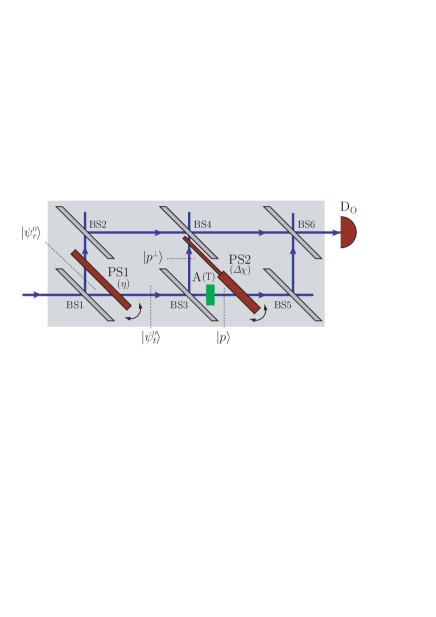
Figure 1: Experimental setup utilizing a double-loop perfect-crystal neutron interferometer: One loop is used for the state manipulation with a phase shifter (PS2) together with a beam attenuator(A) and the other one provides a reference beam with adjustable phase by use of the phase shifter (PS1).

For testing the spatial geometric phase we use a double-loop interferometer (cf. Fig. 1), where the incident (unpolarized) neutron beam $|\psi\rangle$ is split at the beam splitter BS1 into a reflected beam $|\psi_{r}^{0}\rangle$ and a transmitted beam $|\psi_{t}^{0}\rangle$.

The reflected beam $|\psi_{r}^{0}\rangle$ is used as a reference with adjustable relative phase $\eta$ to $|\psi_{t}^{0}\rangle$ due to the phase shifter PS1. The latter beam is defined to be in the state $|\psi_{t}^{0}\rangle\equiv|p\rangle$ before the beam splitter BS3, where $|p\rangle$ is the eigenstate to the operator $P_{p}\equiv|p\rangle\langle p|$ measuring the path. Behind BS3 there are two possible orthogonal paths $|p\rangle$ and $|p^{\perp}\rangle$ spanning a two-dimensional Hilbert space, where $|p\rangle$ denotes the state of the transmitted beam and $|p^{\perp}\rangle$ the state of the reflected beam, respectively. Having a 50:50 beam splitter $|\psi_{t}^{0}\rangle$ is transformed into a superposition of the basis vectors $|p\rangle$ and $|p^{\perp}\rangle$: $|\psi_{t}^{0}\rangle\mapsto|q\rangle\equiv(|p\rangle+|p^{\perp}\rangle)/\sqrt{2}$. The corresponding projection operator $P_{q}\equiv|q\rangle\langle q|=(1+|p\rangle\langle p^{\perp}|+|p^{\perp}\rangle\langle p|)/2$ (and also $P_{q^{\perp}}=1-P_{q}=|q^{\perp}\rangle\langle q^{\perp}|$) measures the interference instead of the paths.

The transmitted beam $|\psi_{t}^{0}\rangle$ is subjected to further evolution in the second loop of the interferometer by use of beam splitters (BS4, BS5 and BS6), an absorber (A) with transmission coefficient $T$ and a phase shifter (PS2) generating a phase shift of $e^{i\chi_{1}}$ on the upper ($|p^{\perp}\rangle$) and $e^{i\chi_{2}}$ on the lower beam path ($|p\rangle$), respectively, yielding the final state $|\psi_{t}\rangle$. Thus, the evolution causing the spatial geometric phase can be written as

$$|\psi_{t}^{0}\rangle \xrightarrow{\text{BS3}} \frac{1}{\sqrt{2}}(|p^{\perp}\rangle+|p\rangle)\xrightarrow{\text{A}}\frac{1}{\sqrt{2}}(|p^{\perp}\rangle+\sqrt{T}|p\rangle)$$

$$\xrightarrow{\text{PS2}} \frac{1}{\sqrt{2}}(e^{i\chi_{1}}|p^{\perp}\rangle+\sqrt{T}e^{i\chi_{2}}|p\rangle)\equiv|\psi_{t}\rangle.$$

The transformation of the reference beam $|\psi_{r}^{0}\rangle$ is given by $|\psi_{r}^{0}\rangle\mapsto e^{i\eta}|\psi_{r}^{0}\rangle\mapsto e^{i\eta}|p^{\perp}\rangle$, which follows from the fact that the path of $|\psi_{r}^{0}\rangle$ coincides with the path of the beam reflected at BS3 labeled by $|p^{\perp}\rangle$.

In the last step $|\psi_{t}\rangle$ and the reference beam are recombined at BS6 and detected in the forward beam at the detector D_O. This recombination can be described by application of the interference projection operator $P_{q}=|q\rangle\langle q|$ to $|\psi_{t}\rangle$ as well as to $|\psi_{r}^{0}\rangle$:

$$|\psi_{t}^{\prime}\rangle \equiv P_{q}{\psi_{t}}=K(e^{i\chi_{1}}+\sqrt{T}e^{i\chi_{2}})|q\rangle$$

$$e^{i\eta}|\psi_{r}^{\prime}\rangle \equiv P_{q}e^{i\eta}{|\psi_{r}^{0}\rangle}=Ke^{i\eta}|q\rangle,$$ (2)

where $K$ is some scaling constant.

The intensity $I$ measured in the detector $D_{O}$ is proportional to the modulus squared of the superposition $|\psi_{t}^{\prime}\rangle+e^{i\eta}|\psi_{r}^{\prime}\rangle$:

$$I \propto \big{|}|\psi_{t}^{\prime}\rangle+e^{i\eta}|\psi_{r}^{\prime}\rangle|^{2}=\langle\psi_{r}^{\prime}|\psi_{r}^{\prime}\rangle+\langle\psi_{t}^{\prime}|\psi_{t}^{\prime}\rangle+$$ (3)

$$+2|\langle\psi_{r}^{\prime}|\psi_{t}^{\prime}\rangle|\cos(\eta-\Phi)$$

with $\Phi\equiv\arg\langle\psi_{r}^{\prime}|\psi_{t}^{\prime}\rangle$. Explicitly, using Eq. (Non-cyclic Geometric Phase due to Spatial Evolution in a Neutron Interferometer) we obtain

$$\Phi = \frac{\chi_{1}+\chi_{2}}{2}+\arg\left(e^{-i\frac{\Delta\chi}{2}}+\sqrt{T}e^{i\frac{\Delta\chi}{2}}\right)$$ (4)

$$= \frac{\chi_{1}+\chi_{2}}{2}-\arctan\left[\tan\left(\frac{\Delta\chi}{2}\right)\left(\frac{1-\sqrt{T}}{1+\sqrt{T}}\right)\right],$$

where $\Delta\chi\equiv\chi_{2}-\chi_{1}$. By varying $\eta$ we can read off $\Phi$ as a shift of the interference pattern.

For our purposes a double loop interferometer is inevitable, since we measure the phase shift generated in one interferometer loop relative to the reference beam, in contrast to a phase difference between two paths measured in usual interferometric setups. Here, the relative phase difference $\Phi$ between $|\psi_{t}^{\prime}\rangle$ and $|\psi_{r}^{\prime}\rangle$ provides information about the evolution of the state $|\psi_{t}^{0}\rangle$ in state space. The geometric phase $\Phi_{g}$ is defined as $\Phi_{g}\equiv\Phi-\Phi_{d}$ Mukunda and Simon (1993), where $\Phi_{d}$ denotes the dynamical part. In our setup $\Phi_{d}$ stems from the phase shifter PS2 and is given by a sum of the phase shifts $\chi_{1}$ and $\chi_{2}$ weighted with the transmission coefficicient $T$ Hasegawa et al. (1996); Wagh (1999), $\Phi_{d}=(\chi_{1}+T\chi_{2})/(1+T)$. It vanishes by an appropriate choice of positive and negative phase shifts in accordance with the transmission, i. e. $\Phi_{d}=0$ for $-\chi_{1}/\chi_{2}=T$.

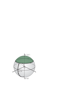
(a) Cyclic evolution

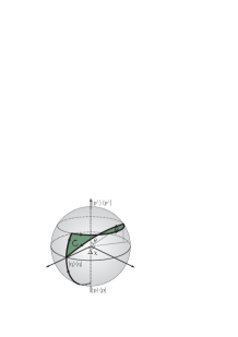
(b) Non-cyclic evolution

Figure 2: Paths on the Bloch-sphere corresponding to the evolution of the state $|\psi_{t}^{0}\rangle$ (a) in the cyclic and (b) non-cyclic case. The enclosed solid angle as seen from the origin of the sphere is proportional to the geometric phase observed in the experiment.

Note, that the same evolution can also be implemented in spin space by thinking of polarizers instead of beam splitters, and magnetic fields instead of absorber and second phase shifter PS2. The phase shift for such a setup differs from $\Phi$ in Eq. (4) merely by a purely dynamical contribution that is compensated in our experiment.

The result from Eq. (4) can also be obtained by purely geometric considerations. Since we are dealing with a two-level system corresponding to the possible paths of $|\psi_{t}^{0}\rangle$ in the second loop of the interferometer the state space is equivalent to a sphere in $\mathbb{R}^{3}$, known as the Bloch-sphere Mittelstaedt et al. (1987); Busch (1987); Hasegawa and Kikuta (1994). From theory we know that the geometric phase $\Phi_{g}$ is given by the (oriented) surface area enclosed by the path of the state vector on the Bloch-sphere and is proportional to the enclosed solid angle as seen from the origin of the sphere.

To each point on the sphere there is a corresponding projection operator. As basis we choose $|p^{\perp}\rangle\langle p^{\perp}|$ and $|p\rangle\langle p|$ represented as the north and the south pole of the sphere, respectively (Fig. 2). At the beam splitter BS3 the state $|\psi_{t}^{0}\rangle$ originating from the point $|p\rangle\langle p|$ is projected to an equal superposition of upper path and lower path depicted as a geodesic from the south pole to the equatorial line on the Bloch-sphere .

The absorber with transmittivity $T=\tan^{2}\theta/2$, $\theta\in[0,\pi/2]$, changes the weights of the superposed basis states $|p\rangle$ and $|p^{\perp}\rangle$. The resulting state is encoded as a point on the geodesic from the north pole to the equatorial line. In particular for no absorption ($\theta=\pi/2$ or $T=1$ ) the state stays on the equator. By inserting a beam block ($\theta=0$ or $T=0$) there is no contribution from $|p\rangle$ so that the state is pinned onto the north pole.

The phase shifter PS2 induces a relative phase shift between the superposing states of $\Delta\chi=\chi_{2}-\chi_{1}$. This corresponds to an evolution along a circle of latitude on the Bloch-sphere with periodicity $2\pi$. The recombination at BS5 followed by the detection of the forward beam in D${}_{\text{O}}$ is represented as a projection to the starting point on the equatorial line, i. e. we have to close the curve associated with the evolution of the state by a geodesic to the point $|q\rangle\langle q|$ in accordance to the results in Samuel and Bhandari (1988).

This evolution path is depicted in Figs. 2(a) and 2(b) for cyclic and non-cyclic evolution, respectively. For a relative phase difference greater than $\pi/2$ we have to take the direction of the loops into account: In Fig. 2(b) the first loop is transversed clockwise, whereas the second loop is transversed counter-clockwise yielding a positive or negative contribution to the geometric phase, respectively.

With this representation we can numerically calculate the solid angle $\Omega$ enclosed by the transversed path on the Bloch-sphere. The resuls obtained in this way for $\Phi_{g}=-\Omega/2$ Berry (1984) are equal to the results based on Eq. (4). This substantiates the emergence of a geometric phase in this type of experiment contrary to other claims Wagh (1999).

As for the experimental demonstration we have used the double-loop perfect-crystal-interferometer installed at the S18 beamline at the high-flux reactor ILL, Grenoble Zawisky et al. (2002). A schematic view of the setup is shown in Fig. 1. Before falling onto the skew-symmetric interferometer the incident neutron beam is collimated and monochromatized by the 220-Bragg reflection of a Si perfect crytal monochromator placed in the thermal neutron guide H25. The wavelength is tuned to give a mean value of $\lambda_{0}=2.715\text{\AA}$. The beam cross-section is confined to $5\times 5\text{mm}^{2}$ and by use of an isothermal box enclosing the interferometer thermal environmental isolation is achieved. As phase shifters parallel sided Al plates are used. In fact, a 5mm-thick plate is taken for the first phase shifter (PS1) inserted in the former loop and plates of different thickness ($d_{1}=0.5$mm and $d_{2}=4.1$mm) are used as the second phase shifter (PS2).

The different thicknesses together with a specific choice of the absorber (A) are to eliminate a phase of unwanted dynamical origin. In each beam a positive phase shift $\chi_{1,2}\propto d_{1,2}$ is induced by PS2 Rauch and Werner (2000). By a rotation of this phase shifter through a (small) angle $\gamma$ about an axis perpendicular to the interferometer $\chi_{1}$ and $\chi_{2}$ change with opposite sign, i. e., $\Delta\chi_{1}\propto-d_{1}\gamma$, while $\Delta\chi_{2}\propto d_{2}\gamma$. For the relative phase shift $\Delta\chi=\chi_{2}-\chi_{1}$ between the two paths we have $\Delta\chi-\chi_{0}\propto(d_{2}+d_{1})\gamma$, where the constant $\chi_{0}$ – determined by the initial position of PS2 – has been adjusted to $\chi_{0}=2n\pi$, $n$ integer, and can thus be neglected.

Furthermore, we have intended to set the transmission coefficients $T_{j}$ of each beam after PS2 and A as $T_{2}/T_{1}=-\Delta\chi_{1}/\Delta\chi_{2}=d_{1}/d_{2}\approx 0.122$ so that the dynamical phase difference between two successive positions of PS2 vanishes. For an appropriate adjustment of the transmission coefficient, we use a gadolinium solution as absorber, which is tuned to exhibit a transmissivity of $T_{\text{abs}}=0.118(5)$. Taking the absorption of the $0.5$mm Al phase shifter into account, a ratio $T_{2}/T_{1}=0.120(5)$ is realized.

The phase shifts $\Phi$ of the sinusoidal intensity modulations due to PS1 are determined at various points on the path traced out by the state, corresponding to a non-cyclic evolution. In practice, this is achieved by measuring the intensity modulation by PS1 at various positions of the PS2 Hasegawa et al. (1996). The parameter of the evolution is the relative phase shift $\Delta\chi$, which was varied from $-0.2\pi$ to $3.0\pi$. The measured phase shift is plotted as the function of $\Delta\chi$ in Fig. 3 together with theoretically predicted curves: one (dotted curve) is obtained by assuming an ideal situation of hundred percent visibility for all loops, whereas the practically diminished visibility is taken into account for the other (solid curve). In particular, the two subbeams from the second loop are only partially overlapping (in space) with the reference beam at BS6 due to unequal spatial displacements caused by the unequal thicknesses of the plates of PS2. These non-overlapping parts do not contribute to the interference pattern that in turn induces a flattening of the measured curve relative to the ideal curve. Other, however minor, contributions to this flattening are from inhomogenous phase distributions and transmission coefficients leading to an incoherent superposition of states. Averaging over such a state distribution gives rise to additional damping terms $e^{-\Gamma_{i}}$ in each beam, i. e. $\Phi^{\prime}=\arg[\sqrt{T_{1}}e^{-\Gamma_{1}}e^{i\chi_{1}}+\sqrt{T_{2}}e^{-\Gamma_{2}}e^{i\chi_{2}}]$ in contrast to $\Phi$ in Eq. (4), which can also be explained in terms of a mixed state geometric phase Sjöqvist et al. (2000).

All the mentioned influences are subsumed in the fit coefficient $C=0.57(2)$ obtained from a least-squares fit (solid line) to the measured data using the function $\arg[\sqrt{T_{1}}e^{-is_{1}\Delta\chi}+C\sqrt{T_{2}}e^{is_{2}\Delta\chi}]$ with $s_{1,2}=d_{1,2}/(d_{1}+d_{2})$, which is a version of Eq. (4) adapted to the experimental situation. Note, that these experimental factors do not invalidate the discussion on the vanishing dynamical phase: The deviation of the experimentally determined (solid) curve from the ideal (dotted) curve is due to the measurement circumstances in the neutron interferometer. The remaining contribution of the dynamical phase due to the slightly different ratios of $-\Delta\chi_{1}/\Delta\chi_{2}$ and $T_{2}/T_{1}$ can be calculated to yield $\Phi_{d}=-0.009(26)$ at $\Delta\chi=2\pi$.

One can recognize the increase of the measured phase shift $\Phi$ in Fig. 3 due to the positively oriented surface on the Bloch-sphere (c.f. Fig. 2(b)) followed by a decrease due to the counter-clockwise transversed loop yielding a negative phase contribution. This behaviour clearly exhibits the geometric nature of the measured phase. For a cyclic evolution ($\Delta\chi=2\pi$) the measured phase is $-0.684(48)$ which is in a good agreement with the analytical value $-0.683$ of the geometric phase for a ratio $-\chi_{1}/\chi_{2}=T_{2}/T_{1}=0.5/4.1$.

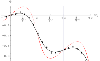
Figure 3: Observed phase shift $\Phi$ for a non-cyclic evolution of the state vector parameterized by the relative phase shift $\Delta\chi$. The dotted line indicates the theoretical prediction for the geometric phase assuming hundred percent visibility, whereas the solid line takes the diminished visibility into account. For a cyclic evolution ($\Delta\chi=2\pi$) we obtain $\Phi_{g}=-0.684(48)$ radians for the transmission ratio $T_{2}/T_{1}=0.120(5)$.

Another indication for a measurement of a non-cyclic geometric phase is the varying amplitude of the interference fringes dependent on $\Delta\chi$Wagh (1999). However, for the absorption ratio $T_{2}/T_{1}=0.122$ these differences are at the detection limit. Measurements of other $T$-values are of interest and detailed results of such measurements will be published in a forthcoming publication.

In summary we have shown that one can ascribe a geometric phase not only to spin evolutions of neutrons, but also to evolutions in the spatial degrees of freedom of neutrons in an interferometric setup. This equivalence is evident from the description of both cases via state vectors in a two dimensional Hilbert space. However, there have been arguments contra the experimental verification in Hasegawa et al. (1996) which we believe can be settled in favour of a geometric phase appearing in the setup described above. The twofold calculations of the geometric phase either in terms of a shift in the interference fringes or via surface integrals in an abstract state space allows for a geometric interpretation of the obtained phase shift. The experiments exhibit a shift of the interference pattern that reflects these theoretical predictions up to influences due to the different visibilities in the different beams.

This research has been supported by the Austrian Science Foundation (FWF), Project Nr. F1513. S. F. wants to thank E. Sjöqvist for valuable discussions and K. Durstberger for critical readings of the manuscript.

References

- Pancharatnam (1956) S. Pancharatnam, Proc. Indian Acad. Sci., Sect. A 44, 247 (1956).
- Berry (1984) M. V. Berry, Proc. R. Soc. Lond. A 392, 45 (1984).
- Wilczek and Zee (1984) F. Wilczek and A. Zee, Phys. Rev. Lett. 52, 2111 (1984).
- Aharonov and Anandan (1987) Y. Aharonov and J. Anandan, Phys. Rev. Lett 58, 1593 (1987).
- Samuel and Bhandari (1988) J. Samuel and R. Bhandari, Phys. Rev. Lett. 60, 2339 (1988).
- Mukunda and Simon (1993) N. Mukunda and R. Simon, Ann. Phys. 228, 205 (1993).
- Pati (1995) A. K. Pati, J. Phys. A 28 2087(1995).
- Manini and Pistolesi (2000) N. Manini and F. Pistolesi, Phys. Rev. Lett. 85, 3067 (2000).
- Uhlmann (1986) A. Uhlmann, Rep. Math. Phys. 24 229 (1986).
- Sjöqvist et al. (2000) E. Sjöqvist, A. K. Pati, A. Ekert, J. S. Anandan, M. Ericsson, D. K. L. Oi, and V. Vedral, Phys. Rev. Lett. 85, 2845 (2000).
- Filipp and Sjöqvist (2003) S. Filipp and E. Sjöqvist, Phys. Rev. Lett. 90 050403(2003).
- Tomita and Chiao (1986) A. Tomita and R. Y. Chiao, Phys. Rev. Lett. 57, 937 (1986).
- Du et al. (2003) J. Du, P. Zou, M. Shi, L. C. Kwek, J.-W. Pan, C. H. Oh, A. Ekert, D. K. L. Oi, and M. Ericsson, Phys. Rev. Lett. 91, 100403 (2003).
- Rauch and Werner (2000) H. Rauch and S. A. Werner, Neutron Interferometry: Lessons in experimental Quantum Mechanics (Clarendon Press, Oxford, 2000).
- Hasegawa et al. (2003) Y. Hasegawa, R. Loidl, G. Badurek, M. Baron, and H. Rauch, Nature 425, 45 (2003).
- Rauch et al. (2002) H. Rauch, H. Lemmel, M. Baron, and R. Loidl, Nature 417, 630 (2002).
- Hasegawa et al. (1996) Y. Hasegawa, M. Zawisky, H. Rauch, and A. I. Ioffe, Phys. Rev. A 53, 2486 (1996).
- Hasegawa et al. (2001) Y. Hasegawa, R. Loidl, M. Baron, G. Badurek, and H. Rauch, Phys. Rev. Lett. 87, 070401 (2001); Y. Hasegawa, R. Loidl, G. Badurek, M. Baron, N. Manini, F. Pistolesi, and H. Rauch, Phys. Rev. A 65, 052111 (2002)
- Wagh (1998) A. G. Wagh, V. C. Rakhecha, P. Fischer, and A. Ioffe, Phys. Rev. Lett. 81, 1992 (1998).
- Bitter and Dubbers (1987) T. Bitter and D. Dubbers, Phys. Rev. Lett. 59, 251 (1987).
- Bertlmann et al. (2004) R. A. Bertlmann, K. Durstberger, Y. Hasegawa, and B. C. Hiesmayr, Phys. Rev. A 69, 032112 (2004).
- Wagh (1999) A. G. Wagh, Phys. Rev. A 59, 1715 (1999).
- Mittelstaedt et al. (1987) P. Mittelstaedt, A. Prieur, and R. Schieder, Found. Phys. 17, 891 (1987).
- Busch (1987) P. Busch, Found. Phys. 17, 905 (1987).
- Hasegawa and Kikuta (1994) Y. Hasegawa and S. Kikuta, Z. Phys. B 93, 133 (1994).
- Zawisky et al. (2002) M. Zawisky, M. Baron, R. Loidl, and H. Rauch, Nucl. Instr. Meth. A 481, 406 (2002).