States for phase estimation in quantum interferometry

Abstract

Ramsey interferometry allows the estimation of the phase $\varphi$ of rotation of the pseudospin vector of an ensemble of two-state quantum systems. For $\varphi$ small, the noise-to-signal ratio scales as the spin-squeezing parameter $\xi$, with $\xi<1$ possible for an entangled ensemble. However states with minimum $\xi$ are not optimal for single-shot measurements of an arbitrary phase. We define a phase-squeezing parameter, $\zeta$, which is an appropriate figure-of-merit for this case. We show that (unlike the states that minimize $\xi$), the states that minimize $\zeta$ can be created by evolving an unentangled state (coherent spin state) by the well-known 2-axis counter-twisting Hamiltonian. We analyse these and other states (for example the maximally entangled state, analogous to the optical “NOON” state $|\psi\rangle=(|N,0\rangle+|0,N\rangle)/\sqrt{2}$) using several different properties, including $\xi$, $\zeta$, the coefficients in the pseudo angular momentum basis (in the three primary directions) and the angular Wigner function $W(\theta,\phi)$. Finally we discuss the experimental options for creating phase squeezed states and doing single-shot phase estimation.

I Introduction

A spin squeezed state (SSS) Kitagawa and Ueda (1993); Wineland et al. (1992) is a collective (entangled) state of many individual spin-systems such that a parameter $\xi^{2}$ is less than unity. The value $\xi^{2}=1$ is known as the standard quantum limit, as it is the value it would have if all of the individual spin vectors were unentangled, and oriented in the same direction: a coherent spin state (CSS) Kitagawa and Ueda (1993); Wineland et al. (1992).

Various authors have suggested that spin squeezed states could improve the precision of various measuring devices Wineland et al. (1992); Kitagawa and Ueda (1993). In particular, there is a reduction of quantum noise in Ramsey interferometry Wineland et al. (1992) by a factor $\xi^{2}$, as verified experimentally by Meyer et al Meyer et al. (2001). One may be inclined to think that the parameter $\xi^{2}$ is the only one that matters for spin squeezed states. Here we argue that its generality has been over stressed.

To be specific, if we wish to use a state for a single-shot measurement of the angle $\varphi$ of rotation of the state around some axis of the Bloch sphere, and there is no prior information about $\varphi$, then the maximally spin-squeezed state is not the best state. This point has been previously made in Ref. Berry et al. (2001). Here we delve into this issue in more detail, defining a new parameter, $\zeta^{2}$, which we call phase-squeezing. We investigate this, $\xi^{2}$, and several other characteristics of the CSS and five different entangled spin-states. Through this we elucidate the relation between concepts such as spin squeezing, phase squeezing, NOON states, and phase estimation.

The states that give optimal single-shot precision were identified in Ref. Berry and Wiseman (2000), where a practical near-optimum single-shot estimation scheme was also proposed. A method for engineering these optimal states for optical interferometry was also suggested in the same reference, but it would be extremely challenging to implement. In this paper we have investigated a more realistic proposal, to produce near optimal states for single shot quantum interferometry in an ensemble of spins using the well-known 2-axis counter-twisting Hamiltonian (2ACT) Kitagawa and Ueda (1993) (also see section III.2) . The results are quite encouraging for the experimental realization of optimal phase-squeezed states, in contrast to the situation for maximally spin-squeezed states.

The structure of this paper is as follows. In Sec. II we review phase estimation by interferometry, and the limitations of $\xi^{2}$ as a figure of merit for this purpose. This motivates our introduction of a new parameter, $\zeta^{2}$. In Sec. III we review the states we wish to consider: coherent spin states, Yurke states, NOON states, optimal phase-squeezed states, 2ACT spin-squeezed states, and 2ACT phase-squeezed states. The last of these is introduced here for the first time. In Sec. IV we quantitatively investigate various properties for each of these states: $\xi^{2}$, $\zeta^{2}$, the canonical phase probability distribution, the state coefficients in the angular momentum basis (in the $x$, $y$, and $z$ directions), and the angular Wigner function $W(\phi,\theta)$. We emphasize the trends that can be seen across the various states, especially using the Wigner function. We conclude in Sec. V with a discussion of the experimental options for creating phase squeezed states and doing near optimal single-shot phase estimation.

II Spin Squeezing and Interferometry

The equivalence between Ramsey interferometry and Mach-Zehnder (MZ) interferometry has been discussed at length Wineland et al. (1994). In the latter case a field is introduced to the input ports of a MZ interferometer, then the interferometer transforms the change in phase in one arm ($\varphi$) to changes in intensity of the field at the output ports. If the $N$ quanta entering the input ports are entangled the minimum detectable phase change scales as $1/N$, the Heisenberg limit Holland and Burnett (1993). This an increase in the signal to noise ratio (SNR) when compared to a non entangled states (e.g. all quanta entering at one port) of order $\sqrt{N}$. The non-entangled scaling of $1/\sqrt{N}$ is known as the standard quantum limit.

Ramsey interferometry also measures a phase $\varphi$: the angle of rotation of all spins about some axis. Spin squeezing, a form of entanglement, enables this phase to be estimated better than the standard quantum limit Wineland et al. (1992). In principle this could enable a better atomic clock, where an initial state is allowed to evolve (rotate) and then the phase is estimated to give a measure of the time elapsed from preparation. We shall now revisit the logic that led to the formulation of the spin squeezing parameter as treated in Wineland et al. (1994).

II.1 Spin Squeezing Parameter $\xi^{2}$

Consider a ensemble of $N$ two level atoms, a spin $J$ system, where $N=2J$. The angular momentum operators are $J_{i}=(1/2)\sum_{k=1}^{N}\sigma_{i}^{k}$ where $\sigma_{i}\in\{x,y,z\}$. For a precision measurement on this system we are interested in the sensitivity of our chosen input state to rotation. Following Wineland et al Wineland et al. (1994), let the mean collective spin of the system be in the $\hat{\textbf{x}}$ direction, i.e. $\langle\vec{J}\rangle=\hat{\textbf{x}}|\langle J_{x}\rangle|$. An interaction between a field and the spin system takes place, causing a rotation in the initial state about the $z$ axis, of $\varphi$.

For $\varphi$ small, its value may be estimate by measuring $J_{y}$, since

$$\langle J_{y}\rangle=|\langle\vec{J}\rangle|\sin{\varphi}.$$ (1)

If $M\gg 1$ measurements of $J_{y}$ are taken, then from the central limit theorem the uncertainty in determining $\varphi$ from the results is $\Delta\varphi=\Delta J_{y}/(\sqrt{M}\partial\langle J_{y}\rangle/\partial\varphi)$. Using Eq. (1) the precision in $\varphi$ is

$$\Delta\varphi=\frac{\Delta J_{y}}{|\langle J\rangle|\cos\varphi\sqrt{M}}.$$ (2)

By inspection the minima of Eq. (2) occur when $\cos\varphi$ is maximized. That is, for $|\varphi|\ll 1$.

Naively one would expect a minimum uncertainty coherent state

$$|\psi\rangle_{\rm coh}=|J,J\rangle_{x}$$ (3)

to be a good state to use for phase estimation as all the spins have their mean spin vectors aligned. Here the notation $|{J,\mu}\rangle_{k}$ indicates the egienstates of $J_{k}$ (where typically $k=x,y,z$) with eigenvalue $\mu$. The result that the CSS gives us is the standard quantum limit (SQL). So a ratio of the uncertainty in the state under examination to the SQL will be defined as the squeezing parameter $\xi$. The uncertainty for the coherent state is $\Delta\varphi_{\rm coh}=(J/2M)^{1/2}/J=1/\sqrt{NM}$. Using this SQL, the squeezing parameter becomes

$$\xi=|\Delta\varphi|/|\Delta\varphi|_{\rm coh}=\sqrt{2J}\frac{\Delta J_{y}}{|\langle\vec{J}\rangle|}.$$ (4)

A system with a parameter $\xi^{2}$ less than unity is spin squeezed and necessarily entangled Wang and Sanders (2003).

Although states with small $\xi^{2}$ are good for estimating a small $\varphi$ from multiple ($M\to\infty$) measurements, they are not necessarily optimal for single-shot measurements, or for measurements where $\varphi$ is not known to be small. Consider the case where $N$ is even so that $J=N/2$ is an integer. Then a state which comes close to minimizing $\xi^{2}$ is the Yurke like state Yurke (1986); Wineland et al. (1994),

$$|\psi\rangle_{\rm yur}=\frac{\sin\alpha}{\sqrt{2}}|J,1\rangle_{y}+\cos\alpha|J,0\rangle_{y}+\frac{\sin\alpha}{\sqrt{2}}|J,-1\rangle_{y}.$$ (5)

The minimum $\xi^{2}\sim\sqrt{2/N}$ is achieved as $\alpha\to 0$. In this limit the state is invariant under a rotation of $\pi$ around the $z$ axis. That is, in a single shot measurement it would be impossible to distinguish between a rotation of $\varphi$ and one of $\varphi+\pi$. An even more extreme example is the so-called NOON states Bollinger et al. (1996), defined as

$$|\psi\rangle_{\rm NOON}=(|J,J\rangle_{z}+|J,-J\rangle_{z})/\sqrt{2}.$$ (6)

These states are so-called because in the field representation the state is described as a superposition of Fock states: $(|{N,0}\rangle+|{0,N}\rangle)/\sqrt{2}$. Like the Yurke states, these states allow a measurement of phase with a sensitivity $O(\sqrt{N})$ times better than a coherent state Bollinger et al. (1996); Huelga et al. (1997). However they are are invariant under a $z$-rotation of $2\pi/N$. Thus, in a single shot $\varphi$ would already have to be known to an accuracy of $O(1/N)$ for these states to be useful at all.

II.2 Phase squeezing parameter $\zeta^{2}$

If we wish to estimate the phase shift $\varphi$ from a single measurement, with no prior information about the phase, the quantity we wish to minimize is the uncertainty in that single shot estimate, not the signal to noise ratio or $\xi$. We consider minimizing the uncertainty in an optimal measurement, which requires a generalized measurement Sanders et al. (1997), (although see Ref. Barnett and Pegg (1990)). If arbitrary unitaries can be implemented (as in a quantum computer) and projective measurements are possible, then such generalized measurements can be done Gardiner et al. (1997). Even without such power (effectively that of a quantum computer), a measurement that performs almost as well as an optimal measurement (on any state) can be achieved by adaptive projective measurements on single spins (or quanta) Berry and Wiseman (2000); Berry et al. (2001).

The optimal or canonical measurement scheme Sanders and Milburn (1995); Sanders et al. (1997) involves projection of the state onto the phase states

$$|J,\phi\rangle=(2J+1)^{-1/2}\sum_{\mu=-J}^{\mu=J}e^{-i\mu\phi}|J,\mu\rangle_{z}.$$ (7)

The probability operator measure (POM) for such phase measurements is

$${E}(\phi)d\phi = \frac{2J+1}{2\pi}|J\phi\rangle\langle J\phi|d\phi$$ (8)

$$= \frac{1}{2\pi}\sum_{\mu,\mu^{\prime}=-J}^{\mu=J}e^{i(\mu-\mu^{\prime})\phi}|J,\mu\rangle_{z}\langle J,\mu^{\prime}|d\phi.$$

Provided there is no prior phase information, such measurements are optimal for all states for which the arguments of the coefficients in the $|{J,\mu}\rangle_{z}$ basis are linear in $\mu$ Holevo (1982) (as, for example, in the phase state $|{J,\phi}\rangle$). This includes all states that have been considered for quantum interferometry. Assuming that the initial state $|{\psi}\rangle$ is oriented in the $x$ direction, the POM (8) defines the probability distribution for $\phi$, the best estimate for the phase shift $\varphi$, via

$$P(\phi)d\phi=\langle\psi|e^{+i\varphi J_{z}}{E}(\phi)e^{-i\varphi J_{z}}|\psi\rangle d\phi.$$ (9)

In the canonical measurement scheme it is sensible, for cyclic variables, to define uncertainty is in terms of the sharpness Berry and Wiseman (2000)

$$S = \langle e^{i(\varphi-\phi)}\rangle=\int d\phi P(\phi)e^{i(\varphi-\phi)}$$ (10)

$$= \sum_{\mu=-J}^{\mu=J}{}_{z}\langle J,\mu+1|\psi\rangle\langle\psi|J,\mu\rangle_{z}.$$ (11)

As long as $|{\psi}\rangle$ is oriented in the $x$ direction, $S$ is real and positive, and it is always less than 1. Unlike the variance, the sharpness respects the periodicity of the phase $\phi$. A state with a $S$ close to 1 has a low phase uncertainty, and vice versa. For such states, the variance of $P(\phi)$, $\int_{\phi_{0}}^{\phi_{0}+2\pi}P(\phi)\phi^{2}d\phi$, is given by the approximate formula

$$V\simeq 2(1-S),$$ (12)

provided that $\phi_{0}$ is not near the peak of $P(\phi)$. (Another variance can be defined using $S$, the Holevo variance Holevo (1982) $S^{-2}-1$ but for our purposes it is simpler to take a quantity linear in $S$.)

Now that we have a measure for phase uncertainty, we can define a new figure of merit, appropriate to a single-shot phase estimate with no prior information:

$$\zeta^{2}=4J(1-S).$$ (13)

Similar measures have been considered before; see for example Hradil and Rehacek (1996). It could also be asked, why not scale this equation with respect to the coherent state i.e.

$$\zeta^{2}_{\rm rc}=(1-S)/(1-S_{\rm coh}).$$ (14)

The reason Eq. (13) was chosen over Eq. (14) is that it is a more elegant definition and with small exceptions, discussed in section IV, the two expressions are equal. That is, $\zeta^{2}\approx 1$ for coherent states.

III States

To obtain a better understanding of phase squeezing and the short comings of spin squeezing a number of properties across six test states will be compared. The test states are a coherent state (3), a Yurke state (5), a NOON state (6), plus three new states we define below in this section: the optimal phase squeezed state, the optimal 2ACT-spin squeezed state, and the optimal 2ACT-phase squeezed state. All of the states considered the mean spin direction is in the $\hat{\textbf{x}}$ or $(\theta,\phi)=(0,\pi)$, with the exception of the NOON state, and all except this state and the coherent state are spin-squeezed states, with ‘squeezing’ in the $\hat{\textbf{y}}$ direction. The properties to be examined across all states include the phase and spin squeezing parameters as a function of the number of particles; the Wigner function; state coefficients; and the phase distribution.

III.1 Optimal Phase Squeezed

The maximally phase squeezed states can be found analytically Berry and Wiseman (2000). These states, that minimize $\zeta^{2}$, are given by

$$|\psi\rangle_{\rm opt}=\frac{1}{\sqrt{J+1}}\sum_{\mu=0}^{2J}\sin\left[\frac{(\mu+1)\pi}{2J+2}\right]|J,\mu\rangle_{z}.$$ (15)

III.2 2ACT Squeezed States

So far we have not been concerned about how to create squeezed states. One of the earliest suggestions was to start with a coherent state $|\psi_{\rm coh}\rangle$ and to evolve according to the so-called two-axis countertwisting (2ACT) [1] Hamiltonian

$$H_{\rm 2ACT}=\hbar\gamma(J_{y}J_{z}+J_{z}J_{y})$$ (16)

Here $\gamma$ is the strength of the interaction (A generalized Hamiltonian for spin squeezing has been devised by Wang and Sanders [7]). This generates the unitary evolution operator

$$U(\nu)=\exp\left[\nu\left(J_{+}^{2}-J_{-}^{2}\right)/8\right].$$ (17)

Here $\nu=4\gamma t$ is a scaled time (we use $\nu$ rather than $\mu$ as in [1] to avoid confusion with the $|J,\mu\rangle$ basis states), and $J_{\pm}=J_{y}\pm iJ_{z}$ are the raising and lowering operators in the $\hat{\textbf{x}}$-direction. This Hamiltonian produces squeezing in the $\hat{\textbf{y}}$-direction, and the mean spin remains aligned along the $\hat{\textbf{x}}$ axis.

As is well known Kitagawa and Ueda (1993), the state

$$|{\psi({\nu})}\rangle=U(\nu)|{\psi_{\rm coh}}\rangle$$ (18)

has a minimum in $\xi$ for an optimal value $\nu=\nu_{\rm ss}$. This is shown in Fig. 1. We denote the state for this value as

$$|{\psi}\rangle_{\rm sss}=|{\psi(\nu_{\rm ss})}\rangle$$ (19)

and call it the 2ACT spin-squeezed state. As we show here (for the first time), this phenomenon also occurs for $\zeta^{2}$. That is, $\zeta$ is minimized for an optimal value $\nu=\nu_{\rm ps}$. We denote the state for this value as

$$|{\psi}\rangle_{\rm pss}=|{\psi(\nu_{\rm ps})}\rangle$$ (20)

and call it the 2ACT phase-squeezed state.

As shown in Fig. 1, the optimal value $\nu_{\rm ps}$ for phase squeezing is less than that for spin-squeezing, $\nu_{\rm ss}$. We have numerically determined the optimal times $\nu$ for these two types of squeezing and plotted the result in Fig. 2. It has been previously shown that $\nu_{\rm ss}$ scales as $\log_{2}(N)/N$ Andre and Lukin (2002) in Stockton et al. (2003). We find specifically that $\nu_{\rm ss}\approx 1.25\log_{2}(N)/N$. As Fig. 2 shows, $\nu_{\rm ps}$ appears to remain smaller than $\nu_{\rm ss}$ even for large $N$, although the scaling law for the former is not known.

As is well known, and as we will show in the next section, the 2ACT spin-squeezed states do not achieve the minimum $\xi^{2}$ for a fixed $N$, and are not close to the states that do. By contrast, we have found that the 2ACT phase-squeezed states are almost identical to the optimal phase squeezed states defined in Eq. (15). As we will show in the next section, the minimum $\zeta^{2}$ from the 2ACT-generated states is practically indistinguishable from the minimum possible $\zeta^{2}$.

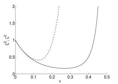
Figure 1: The parameters $\xi^{2}$ (solid line), $\zeta^{2}$ (dashed line) are plotted for the state $|J,-J\rangle$ evolving in time ($\nu=4\gamma t$) under the two axis counter twisting Hamiltonian. $N=20$.

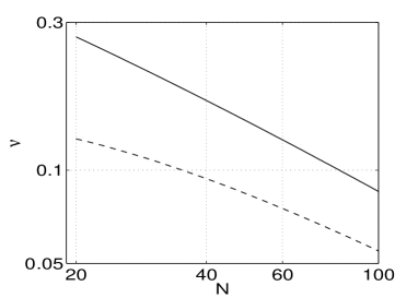
Figure 2: A log log plot of the time ($\nu$) at which the maximal squeezing occurs for phase (dashed line) and spin squeezing (solid line) parameters evolving under the 2ACT.

IV Properties

IV.1 Spin Squeezing

Before discussing $\xi^{2}$ for our various states, we review the simple proof in Ref. Wineland et al. (1994) for a lower bound. Starting with the uncertainty relation

$$\Delta J_{x}\Delta J_{y}\geq\left\langle{J_{z}}\right\rangle^{2}/4$$ (21)

and noting that $\langle J_{y}^{2}\rangle\leq J^{2}$, we get

$$\langle J_{x}^{2}\rangle\geq\frac{\langle J_{z}\rangle^{2}}{4J^{2}}.$$

Now substituting this into Eq. (4) gives

$$\xi^{2}\geq\left(\frac{\langle J_{z}\rangle^{2}}{4J^{2}}\right)\frac{N}{\langle J_{z}\rangle^{2}}\geq\frac{1}{N},$$ (22)

which is sometimes called the Heisenberg limit (HL). There is of course no upper limit on $\xi^{2}$. Note that Sørensen and Mølmer Sorensen and Molmer (2001) produced a definitive paper on maximal squeezing for a state with given $\left\langle{J_{x}}\right\rangle$. The absolute minimum is obtained as $\langle J_{x}\rangle\rightarrow 0$, essentially reproducing the result of Yurke Yurke (1986), which is

$$\xi^{2}=(1+N/2)^{-1}/\cos^{2}\alpha\to 2/N.$$ (23)

where the limit is taking $\alpha\to 0$ and $N\to\infty$.

A plot of $\xi^{2}$ versus $N$ for our test states is shown in Fig. 3. Recall that for a coherent state $\xi^{2}=1$. For all the other states, $\xi^{2}$ scales as $N^{-1}$ for large $N$, but with different coefficients. The worst are the optimal phase squeezed states (which as mentioned above are practically identical to the 2ACT phase squeezed states), for which $\xi^{2}\approx 10/N$ for large $N$. Note also that for $N<5$ the optimal phase-squeezed state is not significantly spin squeezed at all. The NOON state is not included as $\xi$ is undefined for this state.

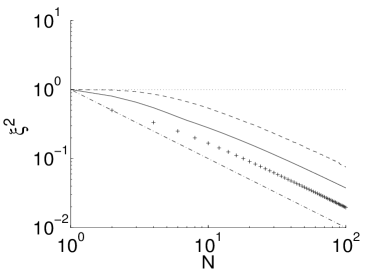
Figure 3: The parameter $\xi^{2}$, plotted for our test states: dotted line for $|{\psi_{\rm coh}}\rangle$, dashed line for $|{\psi_{\rm opt}}\rangle$, solid line for $|{\psi_{\rm sss}}\rangle$, and $+$s for $|{\psi_{\rm yur}}\rangle$ (plotted only for $N$ even). The dash-dotted line is $1/N$.

IV.2 Phase Squeezing

The absolute limit to phase squeezing is easy to analytically obtain as a function of $N$. The maximally phase squeezed states $|{\psi_{\rm opt}}\rangle$ have a sharpness given by Berry et al. (2001)

$$S=\cos\left(\frac{\pi}{N+2}\right).$$ (24)

For large $N$ this gives a phase-squeezing parameter

$$\zeta^{2}\rightarrow\frac{\pi^{2}}{N}.$$ (25)

As a comparison, the case for coherent states will be presented. In the large $\langle J_{x}\rangle$ regime, $J_{y}/J\approx\phi$ and $\langle J_{y}\rangle=0$. For coherent states $\Delta J_{x}=\Delta J_{y}=\sqrt{{J}/{2}}$ so we obtain

$$|\langle e^{i\phi}\rangle| \approx |\langle e^{i{J_{y}}/{J}}\rangle|$$ (26)

$$\approx \langle 1+i\frac{J_{y}}{J}-\frac{1}{2}\frac{J_{y}^{2}}{J^{2}}\rangle$$

$$\approx 1-1/4J.$$

The phase squeezing parameter in the large $N$ limit is thus

$$\zeta^{2}\rightarrow 4J(1-(1-1/4J)=1.$$ (27)

A plot of $\zeta^{2}$ versus $N$ for our test states is shown in Fig. 4. Note that unlike $\xi^{2}$, $\zeta^{2}$ for the coherent state does not exactly equal one — It is noticeably larger than one for states with less than seven particles. For large $N$ it asymptotes to 1 (from above) as expected from the above analysis. From the linearity of Eq. (13) in the state $\rho$, it follows that $\zeta^{2}>1$ for all mixtures of coherent states. Thus $\zeta^{2}<1$ indicates phase squeezing (i.e. better than the standard quantum limit) and hence entanglement (at least for states of well-defined $J$). This is similar to the way $\xi^{2}<1$ indicates spin squeezing and hence entanglement, although that has been shown even for states without well-defined $J$ Sorensen et al. (2001). However, unlike $\xi^{2}$, $\zeta^{2}$ does not drop below 1 even for the optimal state until $N>5$. The large $N$ scaling of $1/N$ is evident for the optimal state, and the 2ACT phase squeezed state gives almost identical results. But in contrast to the $\xi^{2}$ calculation, in this case all other entangled states actually have $\zeta^{2}$ increasing with $N$. For the NOON state $\zeta^{2}=2N$ and for the Yurke state this is very nearly true. This is because of the the symmetry (or near symmetry) of these state implies that the sharpness $S$ is zero for the NOON state and approaches zero for the Yurke state. The result for the 2ACT-SSS will be explained in the next subsection.

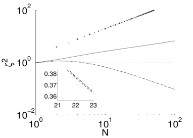
Figure 4: The parameter $\zeta^{2}$, plotted for our test states: dotted line for $|{\psi_{\rm coh}}\rangle$, dashed line for $|{\psi_{\rm opt}}\rangle$, dash-dotted line for $|{\psi_{\rm pss}}\rangle$, solid line for $|{\psi_{\rm sss}}\rangle$, $\bullet$s for $|{\psi_{\rm NOON}}\rangle$ and $+$s for $|{\psi_{\rm yur}}\rangle$ (plotted only for $N$ even). The inset plot is a close up of the same figure showing how close $|{\psi_{\rm pss}}\rangle$ is to $|{\psi_{\rm opt}}\rangle$.

IV.3 Phase distribution

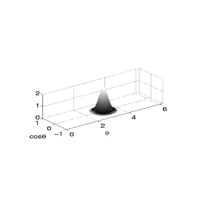
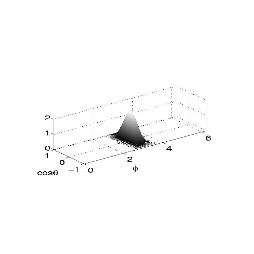
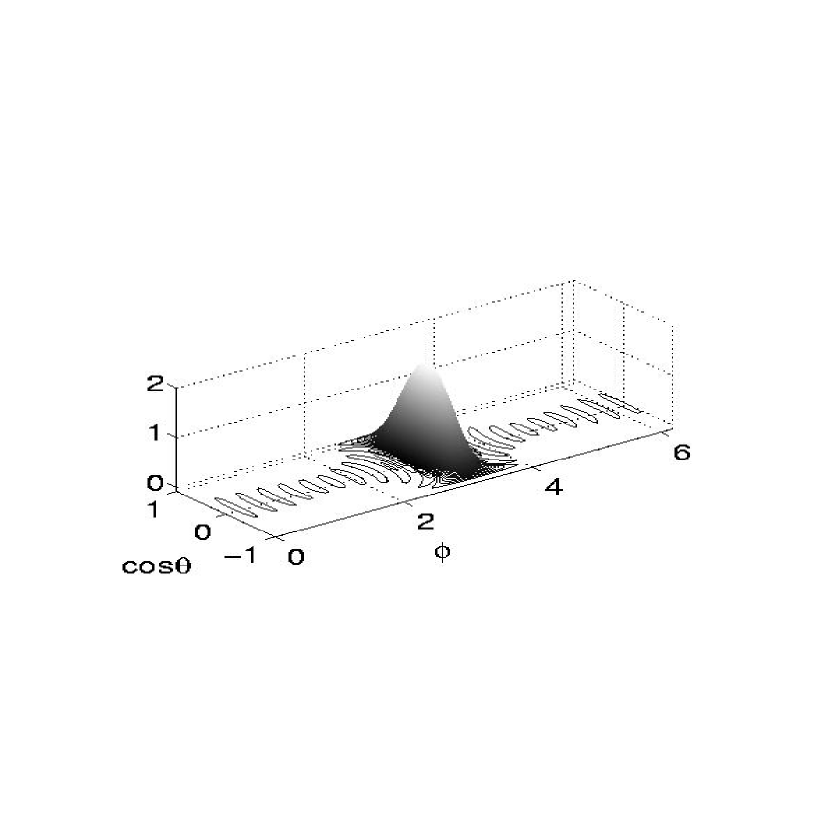
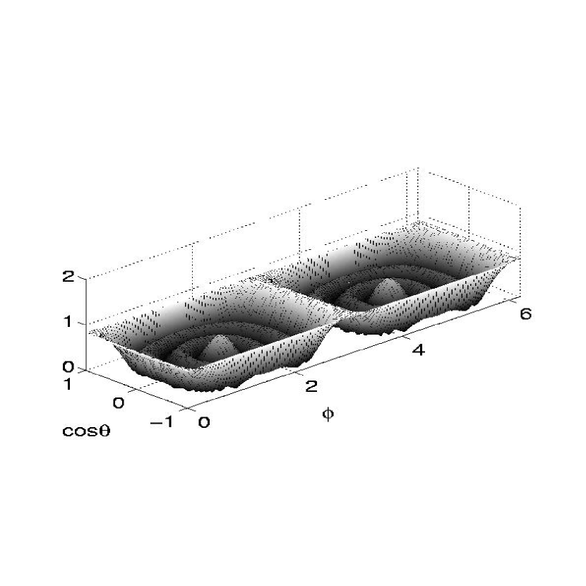
$P(\phi)$

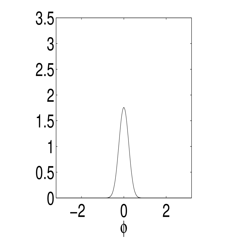
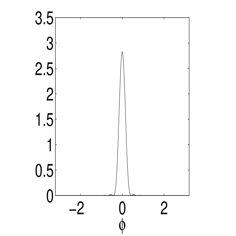
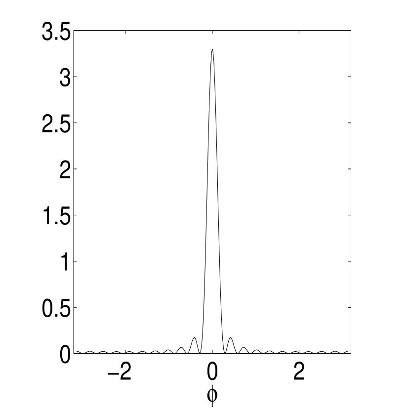
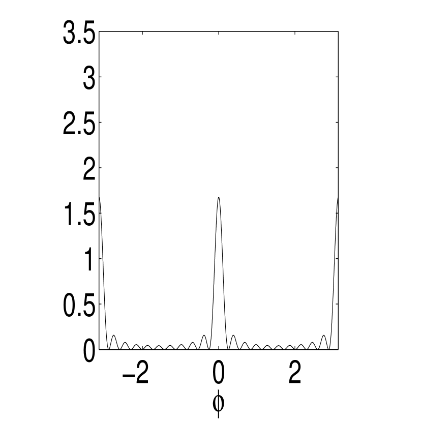
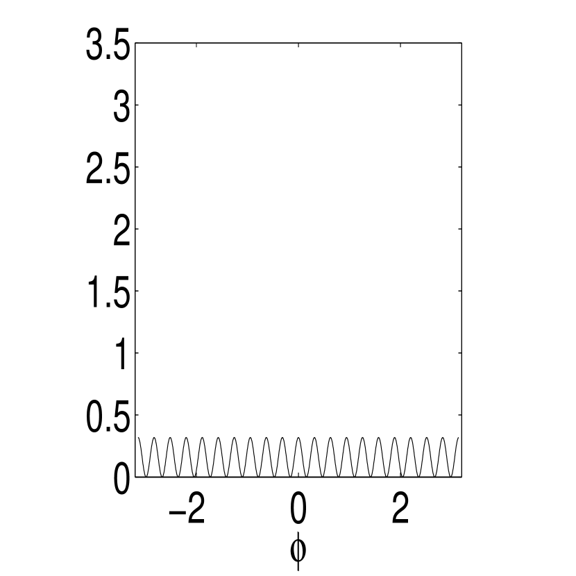
${}_{x}\langle\mu|\psi\rangle$

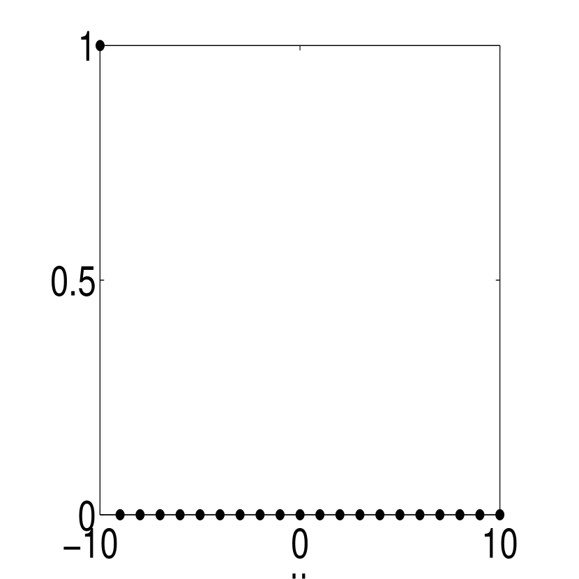
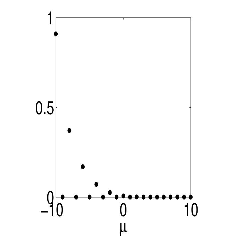
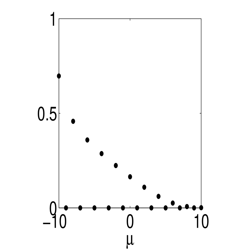
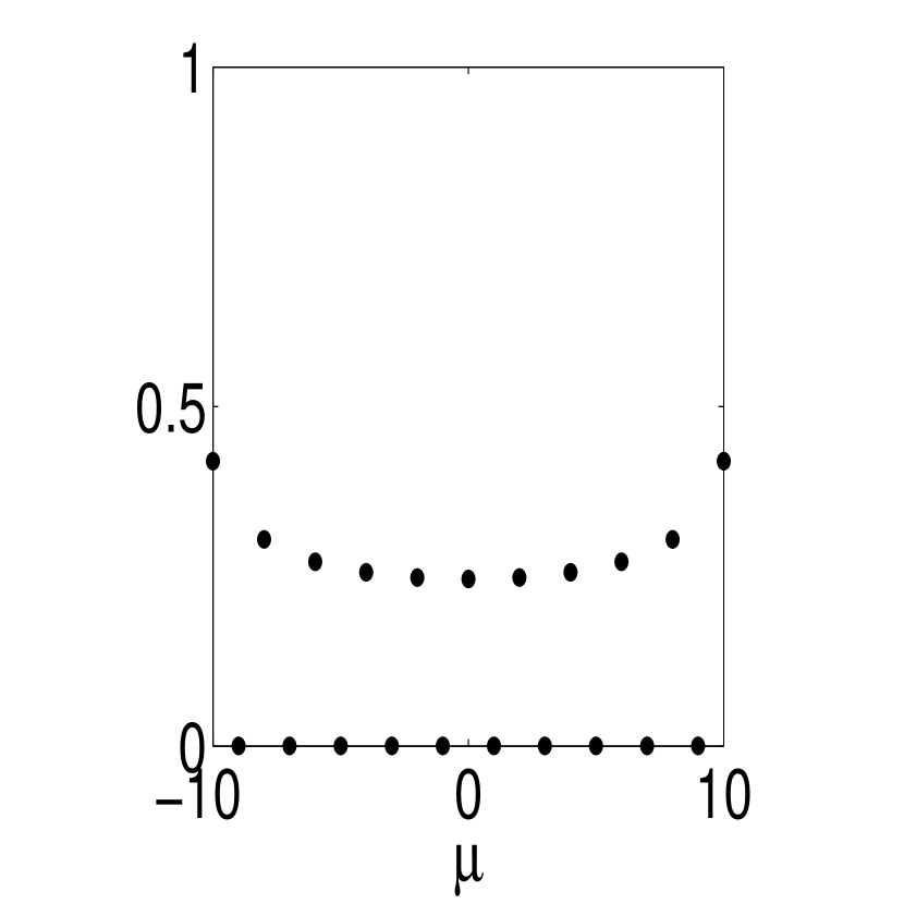
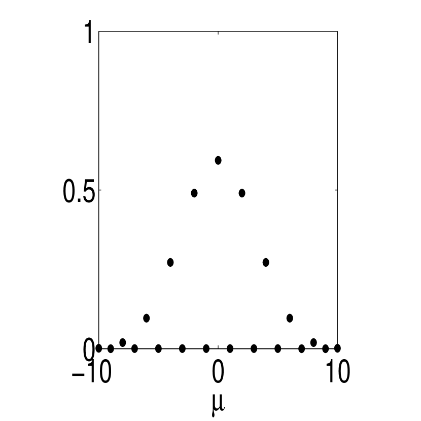
${}_{y}\langle\mu|\psi\rangle$

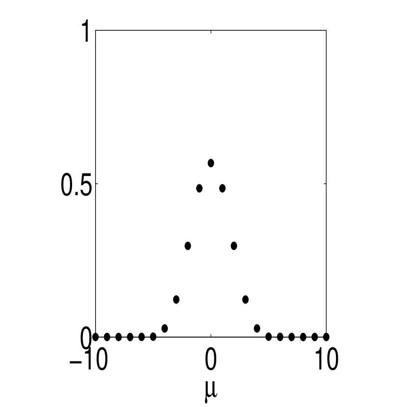
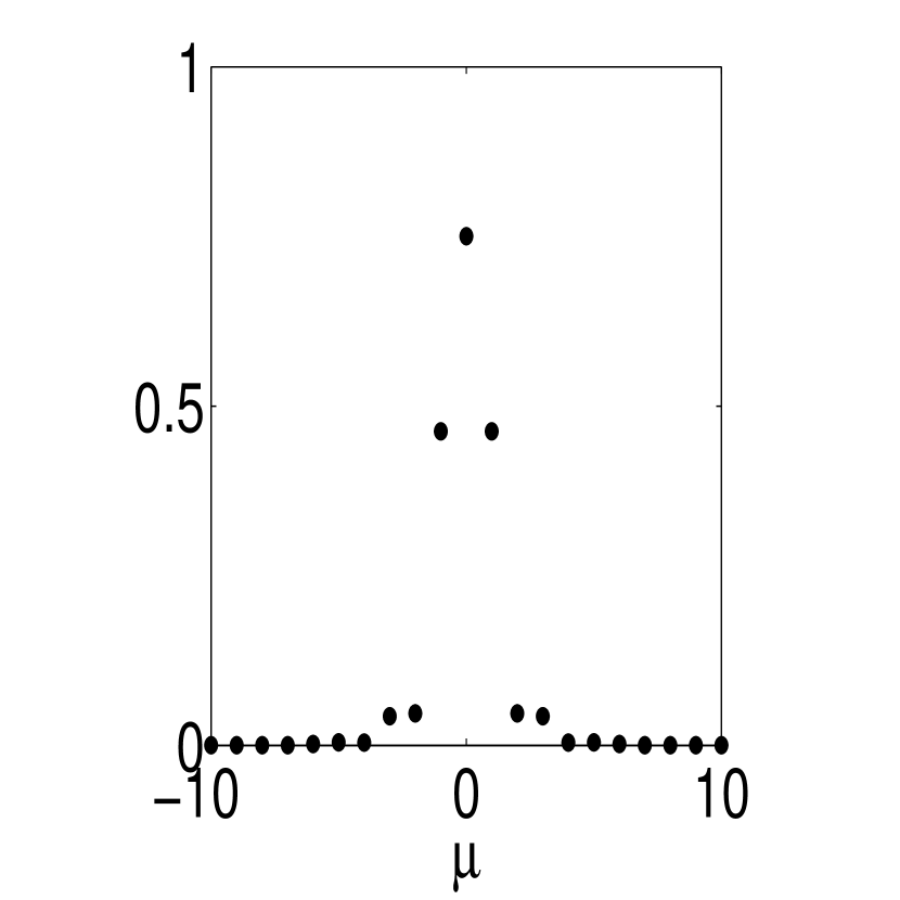
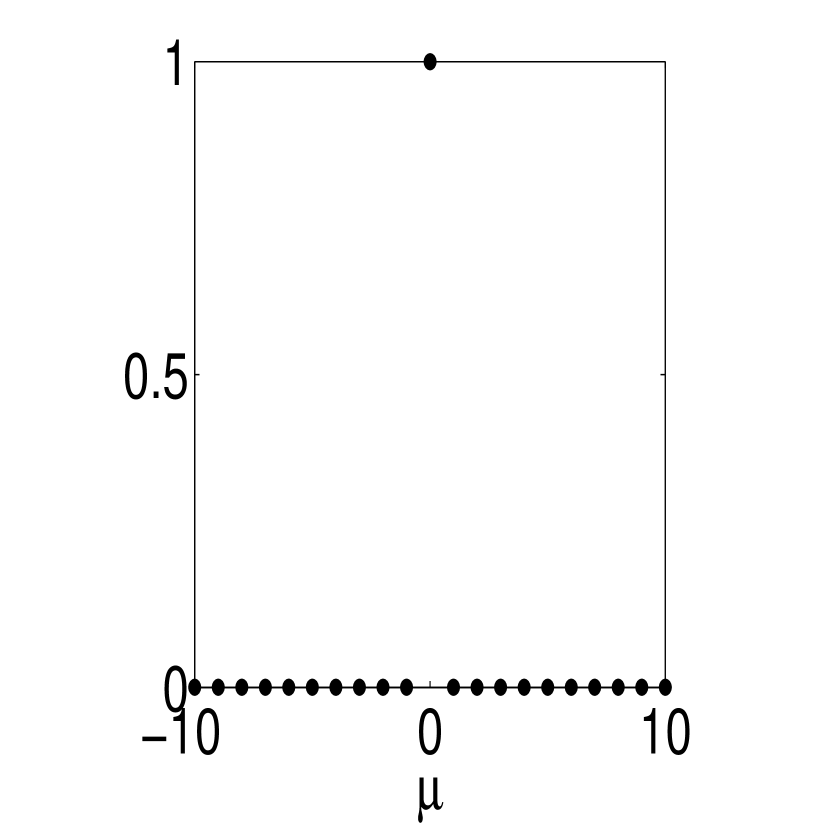
${}_{z}\langle\mu|\psi\rangle$

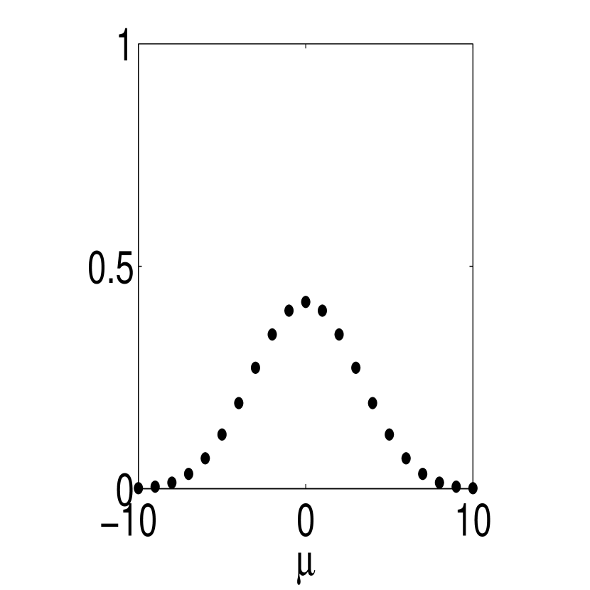
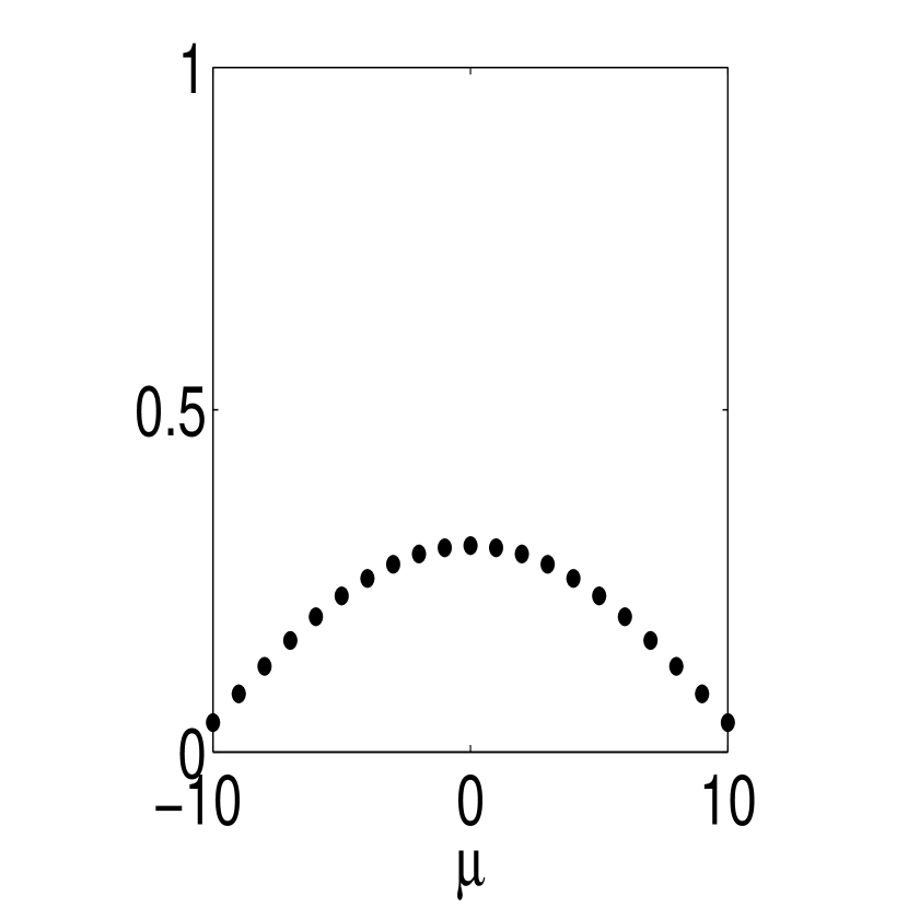
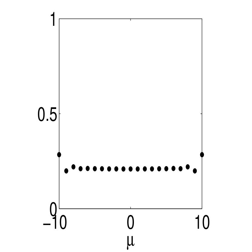
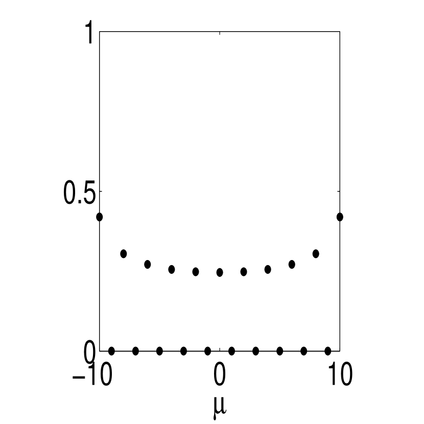
Figure 5: In this figure the five test states (plotted for $N=20$) are in the columns; from left to right: $|{\psi_{\rm coh}}\rangle$ from Eq. (3), $|{\psi_{\rm opt}}\rangle$ from Eq. (15), $|{\psi_{\rm sss}}\rangle$ from Eq. (19), $|{\psi_{\rm yur}}\rangle$ from Eq. (5), and $|{\psi_{\rm NOON}}\rangle$ from Eq. (6). The rows contain the properties of these states that are of interest. The first row is an equal-area plot of the Wigner function $W(\phi,\theta)$, the second is the phase distribution $(\phi,P(\phi))$, while the final three rows are the angular momentum coefficients $\langle J,\mu|\psi\rangle$ in the $x$,$y$ and $z$ directions respectively.

Recall that the phase squeezing parameter $\zeta^{2}$ is a measure of the spread of the phase distribution $P(\phi)$ of an optimal measurement of the phase shift. To understand the results obtained above for $\xi^{2}$ we have plotted $P(\phi)$ as the second row of Fig. 5 with $N=20$. In this figure we have included all our states except $|{\psi_{\rm opt}}\rangle$ as it almost identical to $|{\psi_{\rm pss}}\rangle$.

The coherent state does not contain any surprises — it is quite broad, corresponding to the standard quantum limit. The next state, $|{\psi_{\rm pss}}\rangle$ has a much narrower peak as expected. The third state, $|{\psi_{\rm sss}}\rangle$ has an even narrower central peak but it also has significant side lobes and wings. It is these wings that have such a deleterious effect on the performance of this state in a phase measurement, with $\zeta^{2}$ larger than that for a coherent state. Unlike the first three phase distributions, that of the Yurke state $|{\psi_{\rm yur}}\rangle$ is bimodal. This shows clearly that this state can only determine $\varphi$ modulo $\pi$. Even taking this into account, the side lobes in this distribution (like that of the spin-squeezed state $|{\psi_{\rm sss}}\rangle$) also make this state inferior to the coherent state for single-shot phase estimation, as demonstrated in Ref. Berry et al. (2001). Finally, the NOON state has $N$ peaks, and is the worst state of all in this context, allowing only an estimate of the phase modulo $2\pi/N$.

IV.4 State Coefficients

Again in Fig. 5, the bottom three rows are the state coefficients ${}_{x}\langle\mu|\psi\rangle$, ${}_{y}\langle\mu|\psi\rangle$, and ${}_{y}\langle\mu|\psi\rangle$ respectively. In each case the state has been multiplied by an overall phase factor to ensure that the coefficients are positive. It is instructive to examine the trends (across the states) in the coefficients in the three cardinal directions separately.

For the $x$ coefficients, the coherent state has a single non-zero coefficient, at $\mu=-J$. Moving across, the phase squeezed state develops other non-zero coefficients, and this is further developed in the spin-squeezed states, where the non-zero coefficients stretch almost to $\mu=+J$. In the Yurke state this goes even further, with the coefficients being bimodal, with peaks at $\mu=\pm J$. The NOON state does not fit obviously into this trend, as now there is a single peak at $\mu=0$. In all of these states the coefficients are zero for $\mu$ odd.

For the $y$ coefficients, the trend is even clearer from the coherent state to the Yurke state: an initial symmetric Gaussian-like distribution becomes narrower and narrower until it reaches a single non-zero coefficient at $\mu=0$. Again, the NOON state appears anomalous, being a broad distribution. Note however that unlike those for the other states, these coefficients are zero for $\mu$ odd. In fact, these coefficients are identical to those for the $x$ direction, because the NOON state has no preferred phase.

It is only for the $z$ coefficients that a single trend appears to explain the distribution for all states. To begin, the coherent state has a symmetric Gaussian-like distribution (the same as that for its $y$ coefficients). In opposition to the case of the $y$ coefficients, as the state becomes more phase squeezed, this distribution becomes broader. This is the expected phenomenon of antisqueezing. For the phase squeezed state the distribution is sinusoidal [see Eq. (15)]. For the spin squeezed state it becomes almost flat. Note however that at the ends of the distribution we see the beginning of new trends: the even coefficients are larger than the odd ones, and the largest coefficients are at $\mu=\pm J$. This trend is amplified in the Yurke state, where all odd coefficients are zero, and the curve for the even coefficients is concave up. Finally, in the NOON state it is taken to the extreme where only the $\mu=\pm J$ coefficients are non-zero.

IV.5 Wigner function

The final property we discuss is actually the first one (top row) plotted in Fig. 5: the Wigner function. This is a complete representation of the quantum state, (like the coefficients in a particular direction for a pure state). It has the advantage of showing all the properties of the different states in a dramatic and graphical way.

The spin Wigner function $W(\theta,\phi)$ is a pseudoprobability distribution on the Bloch sphere, with $\theta$ and $\phi$ the usual Euler angles. For spin systems it is defined in Ref. Varilly and Gracia-Bondia (1989) as

$$W(\theta,\phi)={\rm Tr}[\rho\Delta(\theta,\phi)]\\$$ (28)

Here $\theta\in[-\pi/2,\pi/2]$ and $\phi\in[0,2\pi)$ and

$$\Delta(\theta,\phi)=\sum_{\mu,\mu^{\prime}=-J}^{J}Z_{\mu,\mu^{\prime}}(\theta,\phi)|J,\mu\rangle_{z}\langle J,\mu^{\prime}|,$$ (29)

Here

$$Z_{r,s}(\theta,\phi) = \frac{\sqrt{4\pi}}{2j+1}\sum_{l=0}^{2j}\sqrt{2l+1}\langle j,l,r,(s-r)|j,s\rangle$$ (30)

$${\times}\,Y_{l,s-r}(\theta,\phi),$$

where $\langle j,l,r,(s-r)|j,s\rangle$, are Clebsch-Gordan coefficients and $Y_{l,s-r}(\theta,\phi)$ is the usual spherical harmonic function.

We plot the Wigner function using the equal-area projection (described by Euclidean co-ordinates $\phi$ and $\cos\theta$). The original Wigner function Wigner (1932) $W(x,p)$ for position and momentum has the property that the marginal distribution for $x$ is the true position distribution $P(x)$, and likewise for $p$. It might be thought that the marginal distribution $\int_{-1}^{1}d(\cos\theta)W(\phi,\theta)$ should equal the phase distribution $P(\phi)$. Unfortunately this is not the case, as it follows from Ref. Varilly and Gracia-Bondia (1989) that the phase distribution for state $|{\psi}\rangle$ is actually

$$P_{\psi}(\phi)\propto\int_{-1}^{1}d(\cos\theta)d\varphi W_{\psi}(\varphi,\theta)W_{\phi}(\varphi,\theta)$$ (31)

where $W_{\phi}(\varphi,\theta)$ is the Wigner function for a phase state, Eq. (7). Because of the finiteness of the Hilbert space (unlike the $x$-$p$ case), $W_{\phi}(\varphi,\theta)$ is not proportional to $\delta(\varphi-\phi)$. However, for $J$ large it becomes very narrow in $\varphi-\phi$ and so the marginal distribution does approximate the true phase distribution.

In the Wigner representation, the trends are quite clear. The coherent state is approximately Gaussian with standard deviation of order $1/N$. In the optimal state, the distribution is squeezed in $\phi$, and so antisqueezed in $z\propto\cos\theta$. In the optimal 2ACT spin-squeezed state, the phase squeezing has become so pronounced that the antisqueezing has produced a significant disrtribution at $\cos\theta=\pm 1$. This indicates that there is a part of the state in a superposition of $|{J,-J}\rangle_{z}$ and $|{J,J}\rangle_{z}$. This leads to the small ripples in the Wigner function which alternate between positive and negative values (as a function of $\phi$), characteristic of the superposition in the conjugate variable $J_{z}$. This explains the oscillations seen in the wings of the $P(\phi)$ distribution. In the Yurke state the squeezing has become so large that the state has completely wrapped around the Bloch sphere: the distribution is equally weighted at $\phi=0$ and $\phi=\pi$, and also at $\cos\theta=\pm 1$. The ripples are now very pronounced, but not equal in size. Finally, in the NOON state the distribution is confined to $\cos\theta=\pm 1$. The ripples are again very pronounced, and are equal in size, giving the sinusoidal shape of $P(\phi)$ for this state.

V Discussion

We have shown that for single shot measurement about which there is no prior information, the spin squeezing parameter $\xi^{2}$ is not a good figure of merit. This motivated out introduction of a new parameter, $\zeta^{2}$, which we call the phase squeezing. Like $\xi^{2}$, it can scale inversely with the number of particles. We have also shown that the optimal states (minimum $\zeta^{2}$) can be simply produced in an ensemble of spins by starting with a coherent state (all spins pointing in the same direction) under the well-known 2-axis counter-twisting (2ACT) Hamiltonian. This state is different from the optimal state for spin squeezing as produced by this Hamiltonian, which is also different from the globally optimal spin-squeezed states.

There have been a variety of proposals for designing a system with a non linear Hamiltonian Hald et al. (1999); Kuzmich et al. (2000); Sorensen et al. (2001). So far, however the greatest degree of spin (or phase) squeezing observed has been created using quantum measurement and feedback Geremia et al. (2004), as proposed in Refs. Thomsen et al. (2002a, b). As pointed out in Ref. Thomsen et al. (2002b), the feedback produces an effective system Hamiltonian proportional to the 2-axis counter-twisting Hamiltonian. Thus we expect that in the ideal limit feedback based on a QND spin measurement could also produce a state very close to the optimal phase squeezed state. We note that for $N\gg 1$ and moderate degrees of squeezing ($1>\xi^{2}\gg 1/N$), the phase squeezing is identical to the spin squeezing. Finally, it is actually easier to produce optimal phase-squeezed states than optimal spin-squeezed states because it requires a lesser amount of squeezing.

To end, we comment on another method for creating entangled states Kok et al. (2002); Fiurasek (2002) that has recently been implemented experimentally Mitchell et al. (2004). What was done in this experiment was to use “mode mashing” to create a (postselected) NOON state for photons. Specifically, the two polarization modes of each photon play the role of the two spin states. The procedure in this experiment can be very simply modified to produce other entangled states such as Yurke states and optimal phase-squeezed states. At present experiments are limited to $N=3$ photons, for which the advantages of phase squeezed states are minimal. However, it should be possible in the relatively near future to produce a phase squeezed state with $N>5$. Using adaptive measurement techniques Berry and Wiseman (2000); Berry et al. (2001) it would then be possible to perform single shot optical phase estimation substantially better than the standard quantum limit.

Coherent

Phase Squeezed

Spin Squeezed

Yurke

NOON

$W(\theta,\phi)$

References

- Kitagawa and Ueda (1993) M. Kitagawa and M. Ueda, Phys. Rev. A 47, 5138 (1993).
- Wineland et al. (1992) D. J. Wineland, J. J. Bollinger, W. M. Itano, F. L. Moore, and D. J. Heinzen, Phys. Rev. A 46, R6797 (1992).
- Meyer et al. (2001) V. Meyer, M. A. Rowe, D. Kielpinski, C. A. Sackett, W. M. Itano, C. Monroe, and D. J. Wineland, Phys. Rev. Lett. 86, 5870 (2001).
- Berry et al. (2001) D. W. Berry, H. M. Wiseman, and J. K. Breslin, Phys. Rev. A 63, 053804 (2001).
- Berry and Wiseman (2000) D. W. Berry and H. M. Wiseman, Phys. Rev. Lett. 85, 5098 (2000).
- Wineland et al. (1994) D. J. Wineland, J. J. Bollinger, W. M. Itano, and D. J. Heinzen, Phys. Rev. A 50, 67 (1994).
- Holland and Burnett (1993) M. J. Holland and K. Burnett, Phys. Rev. Lett. 71, 1355 1358 (1993).
- Wang and Sanders (2003) X. Wang and B. C. Sanders, arXiv: quant-ph 0302014 (2003).
- Yurke (1986) B. Yurke, Phys. Rev. Lett. 56, 1515 (1986).
- Bollinger et al. (1996) J. J. Bollinger, W. M. Itano, D. J. Heinzen, and D. J. Wineland, Phys. Rev. A 54, R4649 (1996).
- Huelga et al. (1997) S. F. Huelga, C. Macchiavello, T. Pellizzari, A. K. Ekert, M. B. Plenio, and J. I. Cirac, Phys. Rev. Lett. 79, 3865 (1997).
- Sanders et al. (1997) B. C. Sanders, G. J. Milburn, and Z. Zhang, J. of Mod. Opt. 44, 1309 (1997).
- Barnett and Pegg (1990) S. M. Barnett and D. T. Pegg, Phys. Rev. A 41, 3427 (1990).
- Gardiner et al. (1997) S. A. Gardiner, J. I. Cirac, and P. Zoller, Phys. Rev. A 55, 1683 (1997).
- Sanders and Milburn (1995) B. C. Sanders and G. J. Milburn, Phys. Rev. Lett. 75, 2944 (1995).
- Holevo (1982) A. S. Holevo, Probabilistic and Statistical Aspects of Quantum Theory (North-Holland, Amsterdam, 1982).
- Hradil and Rehacek (1996) Z. Hradil and J. Rehacek, Acta. Phys. Slov. 46, 405 (1996).
- Andre and Lukin (2002) A. Andre and M. D. Lukin, Phys. Rev. A 65, 053819 (2002).
- Stockton et al. (2003) J. K. Stockton, J. M. Geremia, A. C. Doherty, and H. Mabuchi, Phys. Rev. A 67, 022112 (2003).
- Sorensen and Molmer (2001) A. S. Sorensen and K. Molmer, Phys. Rev. Lett. 86, 4431 (2001).
- Sorensen et al. (2001) A. Sorensen, L.-M. Duan, J. I. Cirac, and P. Zoller, Nature 409, 63 (2001).
- Varilly and Gracia-Bondia (1989) J. C. Varilly and J. M. Gracia-Bondia, Annals of physics 190, 107 (1989).
- Wigner (1932) E. P. Wigner, Phys. Rev. 40, 749 (1932).
- Hald et al. (1999) J. Hald, J. L. Sorensen, C. Schori, and E. S. Polzik, Phys. Rev. Lett. 83, 1319 (1999).
- Kuzmich et al. (2000) A. Kuzmich, L. Mandel, and N. P. Bigelow, Phys. Rev. Lett. 85, 1594 (2000).
- Geremia et al. (2004) J. M. Geremia, J. K. Stockton, and H. Mabuchi, Science 304, 270 (2004).
- Thomsen et al. (2002a) L. Thomsen, S. Mancini, and H. M. Wiseman, Phys. Rev. A (Rapid Comm.) 65, 061801 (2002a).
- Thomsen et al. (2002b) L. K. Thomsen, S. Mancini, and H. M. Wiseman, J. Phys. B: At. Mol. Opt. Phys. 35, 4937 (2002b).
- Kok et al. (2002) P. Kok, H. Lee, and J. P. Dowling, Phys. Rev. A 65, 052104 (2002).
- Fiurasek (2002) J. Fiurasek, Phys. Rev. A 65, 053818 (2002).
- Mitchell et al. (2004) M. W. Mitchell, J. S. Lundeen, and A. M. Steinberg, Nature 429, 161 (2004).