November 29, 2004

A Simple Scheme to Entangle Distant Qubits from a Mixed State via an Entanglement Mediator

Abstract

A simple scheme to prepare an entanglement between two separated qubits from a given mixed state is proposed. A single qubit (entanglement mediator) is repeatedly made to interact locally and consecutively with the two qubits through rotating-wave couplings and is then measured. It is shown that we need to repeat this kind of process only three times to establish a maximally entangled state directly from an arbitrary initial mixed state, with no need to prepare the state of the qubits in advance or to rearrange the setup step by step. Furthermore, the maximum yield realizable with this scheme is compatible with the maximum entanglement, provided that the coupling constants are properly tuned.

Entanglement is one of the peculiar concepts in quantum physics. It shows a nonlocal property of quantum mechanics, and is the essence of nonclassical phenomena. This concept is now regarded as a key to moving beyond classical ideas and plays a central role in the field of quantum information and computation [1, 2]. The peculiarity of entanglement reveals itself especially when it involves spatially separated systems. Nonlocality has been studied in such situations [3], and such an entanglement is of fundamental importance in quantum communication, for example, quantum teleportation [1, 2].

Practically speaking, an important problem is how to prepare an entanglement between distant parties, and it has been studied for decades [4, 5, 6, 7, 8]. In particular, it is often required to prepare such an entanglement from a (naturally) given state, which is in general a mixed state. Entanglement distillation [2, 9, 10] is therefore an important topic in this context.

A novel mechanism for driving a quantum system from an arbitrary mixed state to a pure state, which makes use of Zeno-like measurements,[11, 12] was discovered recently. This mechanism is that responsible for the following types of behavior: A series of repeated measurements applied to a quantum system can (asymptotically) drive a second system that interacts with the first one into a pure state, even if the second system is initially in an arbitrary mixed state. This provides us with useful procedures for preparing an entanglement between qubits, initialization of multiple qubits, etc. [12, 13]. Furthermore, it has been extended in Ref. ref:qpfes to a scheme to establish an entanglement between distant systems, where measurements are repeated on an “entanglement mediator.”

In this article, we point out that further improvement is possible for the scheme proposed in Ref. ref:qpfes in the case that a single qubit (entanglement mediator) interacts with each of the two (spatially separated) qubits, between which an entanglement is prepared, through a rotating-wave coupling, which is often discussed in the literature [4, 5, 6, 7]. We show in the following that it is indeed possible to obtain a maximally entangled state from an arbitrary mixed state without repeating measurements many times, if the scheme presented in Ref. ref:qpfes is modified properly. In fact, it is found that we actually need only repeat the process (i.e., the interactions of the mediator with the qubits and the measurement of the mediator) three times. Furthermore, the maximum yield attainable in this scheme is shown to be compatible with the maximum entanglement.

We consider two qubits, A and B, which are spatially separated and do not directly interact with each other. In order to make them entangled, another two-level system (the entanglement mediator), X, prepared in a particular state is caused to interact with A and B successively and is measured (Fig. 1).

Figure 1: A scheme for entanglement generation via successive interactions of an entanglement mediator X with qubits A and B.

Such entangling schemes are studied in Ref. ref:Bergou1997, but there it is assumed that the initial states of the distant qubits A and B are prepared in specific pure states. What we show in the following is that no preparation is necessary for A and B. Indeed, a maximally entangled state can be obtained directly from a given (mixed) state within the same (fixed) setup, without introducing other resources or special tunings/arrangements for the initialization of the qubits.

It should be stressed here that the present scheme assumes the application of nonlocal operations of the qubits A and B indirectly through the operations applied to the mediator X, and hence, it is beyond the realm of the entanglement distillation discussed in Refs. ref:QuantInfoCompZeilinger,ref:PurificationBennettPRL1996,ref:TYamamotoNature, etc., which allow only local operations and classical communication.

We assume that the qubits A and B and the entanglement mediator X are two-level systems with a common energy gap $\Omega$ and that each qubit interacts separately with the mediator through a rotating-wave coupling. The free evolution of the three systems is hence described by the Hamiltonian

$$H_{0}=\frac{\Omega}{2}(\sigma_{3}^{\text{(A)}}+\sigma_{3}^{\text{(B)}}+\sigma_{3}^{\text{(X)}}),$$ (1)

and while A (B) interacts with X for a time interval $\tau_{\text{A(B)}}$, the total system evolves according to the Hamiltonian

$$H_{0}+H_{\text{XA(B)}},$$ (2)

with

$$H_{\text{XA}}=g_{\text{A}}(\sigma_{+}^{\text{(X)}}\sigma_{-}^{\text{(A)}}+\sigma_{-}^{\text{(X)}}\sigma_{+}^{\text{(A)}}),$$ (3a)

$$H_{\text{XB}}=g_{\text{B}}(\sigma_{+}^{\text{(X)}}\sigma_{-}^{\text{(B)}}+\sigma_{-}^{\text{(X)}}\sigma_{+}^{\text{(B)}}).$$ (3b)

Here, $\sigma_{i}$ ($i=1,2,3$) are the Pauli operators, and $\sigma_{\pm}=(\sigma_{1}\pm i\sigma_{2})/2$ are the ladder operators. The coupling constant $g_{\text{A(B)}}$ between the qubit A (B) and mediator X is assumed to be an adjustable parameter, but it is fixed throughout the process described in the following.

It is actually possible to initialize A and B in advance, as required in Ref. ref:Bergou1997, without introducing additional resources in the above setup: One can transfer the pure state $|{\uparrow}\rangle$ of X (which is the eigenstate of the operator $\sigma_{3}$ with eigenvalue $+1$) to A (B) by applying the Hamiltonian (2) for an appropriate time interval $g_{\text{A(B)}}\tau_{\text{A(B)}}=\pi/2$, and the qubits are thereby prepared in the pure state $|{\uparrow\uparrow}\rangle_{\text{AB}}$. Note, however, that special arrangements of the values of $g_{\text{A}}\tau_{\text{A}}$ and $g_{\text{B}}\tau_{\text{B}}$, which differ from those necessary for entangling qubits maximally, are required solely for this initialization. It is shown that, without rearranging these parameter values but, rather, fixing them throughout the entire process, we can prepare a maximally entangled state directly from a mixed state in the present scheme.

The idea for obtaining an entanglement from an arbitrary mixed state $\varrho_{\text{AB}}$ is the following. An important point is that the excitation number of qubits

$$N=\frac{1+\sigma_{3}^{\text{(A)}}}{2}+\frac{1+\sigma_{3}^{\text{(B)}}}{2}+\frac{1+\sigma_{3}^{\text{(X)}}}{2}$$ (4)

is a constant of motion, due to the rotating-wave couplings in (3). We first prepare the mediator X in the state $|{\uparrow}\rangle_{\text{X}}$ and let it interact with the qubits A and B successively, through the interactions (3a) and (3b) for the time intervals $\tau_{\text{A}}$ and $\tau_{\text{B}}$, respectively. After these consecutive interactions, the state of X is measured to see whether it has flipped down into the state $|{\downarrow}\rangle_{\text{X}}$. If it has, we know that one and only one of the qubits has certainly flipped from $|{\downarrow}\rangle$ to $|{\uparrow}\rangle$, since the excitation number $N$ given in (4) is conserved in this process. This process, that is, the preparation of X in the state $|{\uparrow}\rangle_{\text{X}}$, the interactions between X and the two qubits A and B, and the projection to $|{\downarrow}\rangle_{\text{X}}$, entails the following state changes of the initial state $\varrho_{\text{AB}}$:

$$\begin{array}[]{ccc}\vskip 6.0pt plus 2.0pt minus 2.0pt|{\uparrow\uparrow}\rangle_{\text{AB}}&\longrightarrow&{\rm disappearing},\\ \vskip 6.0pt plus 2.0pt minus 2.0pt|{\uparrow\downarrow}\rangle_{\text{AB}}\quad\text{and}\quad|{\downarrow\uparrow}\rangle_{\text{AB}}&\longrightarrow&|{\uparrow\uparrow}\rangle_{\text{AB}},\\ |{\downarrow\downarrow}\rangle_{\text{AB}}&\longrightarrow&|{\uparrow\downarrow}\rangle_{\text{AB}}\quad\text{or}\quad|{\downarrow\uparrow}\rangle_{\text{AB}}.\end{array}$$ (5a)

Note that the $$|{\uparrow\uparrow}\rangle_{\text{AB}} \varrho_{\text{AB}} |{\downarrow\downarrow}\rangle_{\text{AB}} |{\uparrow}\rangle_{\text{X}} |{\downarrow}\rangle_{\text{X}} |{\downarrow}\rangle |{\uparrow}\rangle |{\uparrow\uparrow}\rangle_{\text{AB}}$$ component of the initial state is eliminated and the sector becomes vacant after the measurement (projection). Next, a second mediator X prepared in the state is caused to interact with A and B (not necessarily in the same order as the first process), and it is subsequently confirmed again to be in the state . In this second process too, it is possible that the state of only one of the qubits has flipped from to , and the component has thus been eliminated:

$$\begin{array}[]{ccc}\vskip 6.0pt plus 2.0pt minus 2.0pt|{\uparrow\uparrow}\rangle_{\text{AB}}&\longrightarrow&{\rm disappearing},\\ |{\uparrow\downarrow}\rangle_{\text{AB}}\quad\text{and}\quad|{\downarrow\uparrow}\rangle_{\text{AB}}&\longrightarrow&|{\uparrow\uparrow}\rangle_{\text{AB}}.\end{array}$$ (5b)

Now, only the $$|{\uparrow\uparrow}\rangle_{\text{AB}} |{\downarrow\downarrow}\rangle_{\text{AB}} \varrho_{\text{AB}} |{\downarrow\downarrow}\rangle_{\text{AB}} \varrho_{\text{AB}} |{\uparrow\uparrow}\rangle_{\text{AB}} |{\uparrow\uparrow}\rangle_{\text{AB}} |{\downarrow}\rangle_{\text{X}} |{\uparrow}\rangle_{\text{X}} |{\uparrow}\rangle |{\downarrow}\rangle$$ sector is occupied. This was originally the component of the initial state . That is, the state has been extracted from the initial state in the form of , and the qubits A and B have thus been driven to the pure state through these two processes. After this “purification,” the third mediator X prepared in the state is caused to interact with A and B in a prescribed order, and the state is confirmed. This, in turn, flips one of the qubits (but we do not know which one) from to ,

$$\begin{array}[]{ccc}|{\uparrow\uparrow}\rangle_{\text{AB}}&\longrightarrow&|{\uparrow\downarrow}\rangle_{\text{AB}}\quad\text{or}\quad|{\downarrow\uparrow}\rangle_{\text{AB}},\end{array}$$ (5c)

and an entanglement between the distant qubits A and B results. Thus, an entanglement can be obtained from an arbitrary mixed state $\varrho_{\text{AB}}$ after only three measurements, two for the purification and one for the creation of the entanglement. Also, note that this is done with a fixed parameter set, i.e., without readjusting the interaction strengths for the creation of the entanglement. Furthermore, there is no need to repeat these processes many times. Of course, we still need to optimize the processes in order to create an entanglement efficiently, as is clarified below.

There are several possible recipes for this entanglement preparation, because we have the freedom to choose the order in which the mediator X interacts with the qubits A and B for each process. Actually, there are essentially four combinations of such orders. (We can fix the order of the interactions with the mediator in the last process without loss of generality. Then, we are left with two choices for the first mediator, and two choices for the second.) The important point here is to understand which recipe (i.e., the combination of orders of the interactions) enables us to obtain a highly entangled state with a high yield. In the present scheme described in the preceding paragraph, every one of the three measurements applied to the entanglement mediators extracts the correct outcome, and they therefore produce an entangled state with certainty. This is due to the existence of the conserved quantity $N$ given in (4), according to which all states are classified into four sectors with different values of $N$, namely $N=0,1,2$, and $3$, and to the combination of three measurements (projections), which only one of the sectors survives. However, we still need to clarify which combination of orders is the most efficient one, in the sense that the desired results are realized with high probability, and at the same time, a highly entangled state (i.e., a state whose concurrence [16] is close to unity) is obtained.

Figure 2: A recipe for optimal entanglement preparation. The first mediator moves rightward (I), the second one moves leftward (II), and the last one moves rightward (III). (Here, “rightward” means that the interaction between X and A is followed by that between X and B, and “leftward” means that the order is opposite.) If the mediators are found to be in the states indicated in this figure, the processes (I)–(III), represented by the operators $R_{+}$, $L_{+}$, and $R_{-}$, respectively, extract a specific (entangled) state of the qubits A and B. The strength of the interaction between X and A (B) is fixed $g_{\text{A(B)}}\tau_{\text{A(B)}}$ throughout the processes (I)–(III).

It is elementary to confirm that the optimal preparation of a maximally entangled state is possible via the recipe presented in Fig. 2. In the situation depicted there, an appropriate choice of the parameters $g_{\text{A}}\tau_{\text{A}}$ and $g_{\text{B}}\tau_{\text{B}}$ enables us to obtain a maximally entangled state (with concurrence $1$) with the maximum yield realizable in the present scheme. The mediator X is first allowed to travel rightward, that is, to interact with the qubit A and then B. If it is found to be in the state $|{\downarrow}\rangle_{\text{X}}$ after the interactions with A and B on the right, the state of A and B changes according to

$$\varrho_{\text{AB}}\to R_{+}\varrho_{\text{AB}}R_{+}^{\dagger}/\mathop{\text{Tr}}\nolimits_{\text{AB}}(R_{+}\varrho_{\text{AB}}R_{+}^{\dagger}),$$ (6)

where

$$R_{+} \equiv{}_{\text{X}}\langle{\downarrow}|e^{-iH_{\text{XB}}\tau_{\text{B}}}e^{-iH_{\text{XA}}\tau_{\text{A}}}|{\uparrow}\rangle_{\text{X}}$$

$$={-i}\,\Bigl{[}\mathop{\text{s}}\nolimits_{\text{A}}|{\uparrow}\rangle_{\text{A}}\langle{\downarrow}|\otimes\Bigl{(}|{\downarrow}\rangle_{\text{B}}\langle{\downarrow}|+\mathop{\text{c}}\nolimits_{\text{B}}|{\uparrow}\rangle_{\text{B}}\langle{\uparrow}|\Bigr{)}+\mathop{\text{s}}\nolimits_{\text{B}}\,\Bigl{(}|{\uparrow}\rangle_{\text{A}}\langle{\uparrow}|+\mathop{\text{c}}\nolimits_{\text{A}}|{\downarrow}\rangle_{\text{A}}\langle{\downarrow}|\Bigr{)}\otimes|{\uparrow}\rangle_{\text{B}}\langle{\downarrow}|\Bigr{]}$$ (7)

in the interaction picture. (Here, $\mathop{\text{s}}\nolimits_{\text{A}}\equiv\sin g_{\text{A}}\tau_{\text{A}}$, $\mathop{\text{c}}\nolimits_{\text{A}}\equiv\cos g_{\text{A}}\tau_{\text{A}}$, etc.) The second and third mediators are translated leftward and rightward, as depicted in Fig. 2, and as a result, the state of the qubits A and B changes further. The relevant operators read

$$L_{+} \equiv{}_{\text{X}}\langle{\downarrow}|e^{-iH_{\text{XA}}\tau_{\text{A}}}e^{-iH_{\text{XB}}\tau_{\text{B}}}|{\uparrow}\rangle_{\text{X}}$$

$$={-i}\,\Bigl{[}\mathop{\text{s}}\nolimits_{\text{A}}|{\uparrow}\rangle_{\text{A}}\langle{\downarrow}|\otimes\Bigl{(}|{\uparrow}\rangle_{\text{B}}\langle{\uparrow}|+\mathop{\text{c}}\nolimits_{\text{B}}|{\downarrow}\rangle_{\text{B}}\langle{\downarrow}|\Bigr{)}+\mathop{\text{s}}\nolimits_{\text{B}}\,\Bigl{(}|{\downarrow}\rangle_{\text{A}}\langle{\downarrow}|+\mathop{\text{c}}\nolimits_{\text{A}}|{\uparrow}\rangle_{\text{A}}\langle{\uparrow}|\Bigr{)}\otimes|{\uparrow}\rangle_{\text{B}}\langle{\downarrow}|\Bigr{]}$$ (8)

and

$$R_{-} \equiv{}_{\text{X}}\langle{\uparrow}|e^{-iH_{\text{XB}}\tau_{\text{B}}}e^{-iH_{\text{XA}}\tau_{\text{A}}}|{\downarrow}\rangle_{\text{X}}$$

$$={-i}\,\Bigl{[}\mathop{\text{s}}\nolimits_{\text{A}}|{\downarrow}\rangle_{\text{A}}\langle{\uparrow}|\otimes\Bigl{(}|{\uparrow}\rangle_{\text{B}}\langle{\uparrow}|+\mathop{\text{c}}\nolimits_{\text{B}}|{\downarrow}\rangle_{\text{B}}\langle{\downarrow}|\Bigr{)}+\mathop{\text{s}}\nolimits_{\text{B}}\,\Bigl{(}|{\downarrow}\rangle_{\text{A}}\langle{\downarrow}|+\mathop{\text{c}}\nolimits_{\text{A}}|{\uparrow}\rangle_{\text{A}}\langle{\uparrow}|\Bigr{)}\otimes|{\downarrow}\rangle_{\text{B}}\langle{\uparrow}|\Bigr{]}.$$ (9)

The sequence of these three processes thereby extracts a state of the qubits A and B as

$$\varrho_{\text{AB}}\to\tilde{\varrho}_{\text{AB}}=\mathcal{V}\varrho_{\text{AB}}\mathcal{V}^{\dagger}/P,$$ (10a)

with the operator

$$\mathcal{V}\equiv R_{-}L_{+}R_{+}.$$ (10b)

Note that we retain only those events for which the correct states are observed on the mediators; other events are discarded. This is why the states (6) and (10) are renormalized, and the normalization constant,

$$P\equiv\mathop{\text{Tr}}\nolimits_{\text{AB}}(\mathcal{V}\varrho_{\text{AB}}\mathcal{V}^{\dagger}),$$ (11)

is the probability for the entire process depicted in Fig. 2 to be carried out successfully.

The operator $\mathcal{V}$ for this scenario reads

$$\mathcal{V}=2i\mathop{\text{s}}\nolimits_{\text{A}}\mathop{\text{c}}\nolimits_{\text{A}}\mathop{\text{s}}\nolimits_{\text{B}}\,\Bigl{(}\mathop{\text{c}}\nolimits_{\text{A}}\mathop{\text{s}}\nolimits_{\text{B}}|{\uparrow\downarrow}\rangle_{\text{AB}}+\mathop{\text{s}}\nolimits_{\text{A}}|{\downarrow\uparrow}\rangle_{\text{AB}}\Bigr{)}\,{}_{\text{AB}}\langle{\downarrow\downarrow}|,$$ (12)

which clearly shows that it extracts the $|{\downarrow\downarrow}\rangle_{\text{AB}}$ component of the initial state $\varrho_{\text{AB}}$ and converts it into the pure entangled state

$$|{\Psi}\rangle_{\text{AB}}=\frac{1}{\sqrt{1-\mathop{\text{c}}\nolimits_{\text{A}}^{2}\mathop{\text{c}}\nolimits_{\text{B}}^{2}}}\,\Bigl{(}\mathop{\text{c}}\nolimits_{\text{A}}\mathop{\text{s}}\nolimits_{\text{B}}|{\uparrow\downarrow}\rangle_{\text{AB}}+\mathop{\text{s}}\nolimits_{\text{A}}|{\downarrow\uparrow}\rangle_{\text{AB}}\Bigr{)},$$ (13)

i.e.,

$$\varrho_{\text{AB}}\to\tilde{\varrho}_{\text{AB}}=|{\Psi}\rangle_{\text{AB}}\langle{\Psi}|,$$ (14)

and the yield of this entangled state is given by

$$P=4\mathop{\text{s}}\nolimits_{\text{A}}^{2}\mathop{\text{c}}\nolimits_{\text{A}}^{2}\mathop{\text{s}}\nolimits_{\text{B}}^{2}(1-\mathop{\text{c}}\nolimits_{\text{A}}^{2}\mathop{\text{c}}\nolimits_{\text{B}}^{2})\,{}_{\text{AB}}\langle{\downarrow\downarrow}|\varrho_{\text{AB}}|{\downarrow\downarrow}\rangle_{\text{AB}}.$$ (15)

The concurrence[16] of the generated entangled state $|{\Psi}\rangle_{\text{AB}}$ in (13) is readily estimated to be

$$C=\frac{2|\mathop{\text{s}}\nolimits_{\text{A}}\mathop{\text{c}}\nolimits_{\text{A}}\mathop{\text{s}}\nolimits_{\text{B}}|}{\mathop{\text{s}}\nolimits_{\text{A}}^{2}+\mathop{\text{c}}\nolimits_{\text{A}}^{2}\mathop{\text{s}}\nolimits_{\text{B}}^{2}},$$ (16)

from which we see that $C$ is unity if and only if the parameters $g_{\text{A}}\tau_{\text{A}}$ and $g_{\text{B}}\tau_{\text{B}}$ are adjusted to satisfy the condition

$$\tan^{2}\!g_{\text{A}}\tau_{\text{A}}=\sin^{2}\!g_{\text{B}}\tau_{\text{B}};$$ (17)

i.e., a maximally entangled state can be generated by tuning the parameters properly. Furthermore, if they are tuned to satisfy

$$\tan^{2}\!g_{\text{A}}\tau_{\text{A}}=\sin^{2}\!g_{\text{B}}\tau_{\text{B}}=1,$$ (18)

the maximally entangled state is obtained with yield $P={}_{\text{AB}}\langle{\downarrow\downarrow}|\varrho_{\text{AB}}|{\downarrow\downarrow}\rangle_{\text{AB}}$, which is the maximum realizable in the present scheme. This means that the entire component of $|{\downarrow\downarrow}\rangle_{\text{AB}}$ contained in the initial state $\varrho_{\text{AB}}$ is fully extracted and converted into the maximally entangled state $|{\Psi}\rangle_{\text{AB}}$. Even from the maximally mixed state $\varrho_{\text{AB}}=\openone_{\text{AB}}/4$, the maximally entangled state $|{\Psi}\rangle_{\text{AB}}$ can be prepared with a nonvanishing yield, $P=1/4$. The optimal preparation of the maximally entangled state between the distant qubits with $C=1$ and $P={}_{\text{AB}}\langle{\downarrow\downarrow}|\varrho_{\text{AB}}|{\downarrow\downarrow}\rangle_{\text{AB}}$ is thus demonstrated to be possible through only three sequences of consecutive interactions of the mediator X with the qubits A and B. The parameter dependences of the concurrence $C$ and the yield $P$ are plotted in Fig. 3.

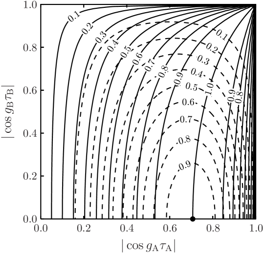
Figure 3: Contour plots of the concurrence $C$ (solid curves) and the yield $P$ (divided by ${}_{\text{AB}}\langle{\downarrow\downarrow}|\varrho_{\text{AB}}|{\downarrow\downarrow}\rangle_{\text{AB}}$) (dashed curves) as functions of $g_{\text{A}}\tau_{\text{A}}$ and $g_{\text{B}}\tau_{\text{B}}$ for the preparation of the entangled state $|{\Psi}\rangle_{\text{AB}}$ through the processes depicted in Fig. 2. In this case, $C$ and $P$ are functions of $|\cos g_{\text{A}}\tau_{\text{A}}|$ and $|\cos g_{\text{B}}\tau_{\text{B}}|$. The optimal entanglement preparation with $C=1$ and $P={}_{\text{AB}}\langle{\downarrow\downarrow}|\varrho_{\text{AB}}|{\downarrow\downarrow}\rangle_{\text{AB}}$ is realized at the point $(|\cos g_{\text{A}}\tau_{\text{A}}|,|\cos g_{\text{B}}\tau_{\text{B}}|)=(1/\sqrt{2},0)$, indicated by the dot.

Similar analyses show that the combinations of the directions (i.e., the order of the interactions in each process) other than that depicted in Fig. 2 do not provide the optimal scheme, and the maximum concurrence and the maximum yield are not simultaneously realizable. Note again that the parameters $g_{\text{A}}\tau_{\text{A}}$ and $g_{\text{B}}\tau_{\text{B}}$ are fixed throughout all the processes. If it is allowed to vary these parameters step by step, more efficient schemes can be constructed. In particular, if the qubits A and B are initialized in the state $|{\uparrow\uparrow}\rangle_{\text{AB}}$ in advance, as described above, the first two steps in the present scheme are not necessary. The present scheme is, however, useful in such a situation that it is not easy to experimentally initialize the system, because it is still possible to prepare a maximally entangled state directly from a given mixed state, with a fixed setting. The scheme that is optimal in any given case depends on the actual experimental setups and experimental feasibility.

The present scheme makes use of the fact that the interactions given in (3) preserve the excitation number $N$ given in (4). Such interactions are found in the literature in the context of quantum information and computation. For example, generation of entanglement (from a specific pure state) was demonstrated in a cavity QED experiment [4], in which a cavity mode plays a role similar to that of the mediator X, and the cavity-atom interaction preserves the excitation number of the atomic qubits and the cavity mode. For long-range entanglement, it is quite likely that a photon could act as the mediator X. In connection to this point, the interaction between a circularly-polarized photon and a $\Lambda$-type atom was recently proposed in this role[17]. Although this interaction, between a photon and an atom, is not precisely the interaction considered here, it also preserves the excitation number and is a potential system to be used in the experimental implementation of the present scheme. Applied to such systems, the present scheme would provide a method of entangling spatially separated qubits. With the goal of realizing such an experiment, we should clarify the effects of decoherence of the mediator X, which may travel a long distance between the qubits A and B, and other possible disturbances on the qubits during the process. Investigations of these points are now in progress.

References

- [1] M. A. Nielsen and I. L. Chuang, Quantum Computation and Quantum Information (Cambridge University Press, Cambridge, 2000).
-
[2]
The Physics of Quantum Information, ed. D.
Bouwmeester, A. Ekert and A. Zeilinger
(Springer-Verlag, Heidelberg, 2000).
C. H. Bennett and D. P. DiVincenzo, \JLNature (London),404,2000,247.
A. Galindo and M. A. Martin-Delgado, \JLRev. Mod. Phys.,74,2002,347. - [3] A. Peres, Quantum Theory: Concepts and Methods (Kluwer Academic Publishers, Dordrecht, 1995).
-
[4]
E. Hagley, X. Maître, G. Nogues, C. Wunderlich, M. Brune,
J. M. Raimond and S. Haroche, \PRL79,1997,1.
J. M. Raimond, M. Brune and S. Haroche, \JLRev. Mod. Phys.,73,2001,565. -
[5]
J. A. Bergou and M. Hillery, \PRA55,1997,4585.
A. Messina, \JLEur. Phys. J. D,18,2002,379.
D. E. Browne and M. B. Plenio, \PRA67,2003,012325. -
[6]
C. Cabrillo, J. I. Cirac, P. García-Fernández and P. Zoller,
\PRA59,1999,1025.
L.-M. Duan, M. D. Lukin, J. I. Cirac and P. Zoller, \JLNature (London),414,2001,413.
D. E. Browne, M. B. Plenio and S. F. Huelga, \PRL91,2003,067901. -
[7]
X.-L. Feng, Z.-M. Zhang, X.-D. Li, S.-Q. Gong and Z.-Z. Xu,
\PRL90,2003,217902.
L.-M. Duan and H. J. Kimble, \PRL90,2003,253601. - [8] R. Ursin, T. Jennewein, M. Aspelmeyer, R. Kaltenbaek, M. Lindenthal, P. Walther and A. Zeilinger, \JLNature (London),430,2004,849.
-
[9]
C. H. Bennett, G. Brassard, S. Popescu, B. Schumacher, J. A. Smolin
and W. K. Wootters, \PRL76,1996,722 [Errata; 78 (1997), 2031].
C. H. Bennett, D. P. DiVincenzo, J. A. Smolin and W. K. Wootters, \PRA54,1996,3824. -
[10]
T. Yamamoto, M. Koashi, Ş. K. Özdemir and N. Imoto,
\JLNature (London),421,2003,343.
Z. Zhao, T. Yang, Y.-A. Chen, A.-N. Zhang and J.-W. Pan, \PRL90,2003,207901.
A. Vaziri, J.-W. Pan, T. Jennewein, G. Weihs and A. Zeilinger, \PRL91,2003,227902. - [11] H. Nakazato, T. Takazawa and K. Yuasa, \PRL90,2003,060401.
- [12] H. Nakazato, M. Unoki and K. Yuasa, \PRA70,2004,012303.
- [13] L.-A. Wu, D. A. Lidar, and S. Schneider, \PRA70,2004,032322.
-
[14]
See, for example,
B. Misra and E. C. G. Sudarshan, \JMP18,1977,756.
H. Nakazato, M. Namiki and S. Pascazio, \JLInt. J. Mod. Phys. B,10,1996,247.
D. Home and M. A. B. Whitaker, \JLAnn. of Phys.,258,1997,237.
P. Facchi and S. Pascazio, in Progress in Optics, ed. E. Wolf (Elsevier, Amsterdam, 2001), Vol. 42, p. 147. - [15] G. Compagno, A. Messina, H. Nakazato, A. Napoli, M. Unoki and K. Yuasa, \PRA70,2004,052316.
- [16] W. K. Wootters, \PRL80,1998,2245.
-
[17]
W. Lange and H. J. Kimble, \PRA61,2000,063817.
J. Hong and H.-W. Lee, \PRL89,2002,237901.
B. Sun, M. S. Chapman and L. You, \PRA69,2004,042316.