Preparation of arbitrary qutrit state based on biphotons

Abstract

The novel experimental realization of three-state optical quantum systems is presented. We use the polarization state of biphotons,propagating in single frequency- and spatial mode, to generate an arbitrary qutrits. In particular the specific sequence of states that are used in the extended version of BB84 quantum key distribution protocol was generated and tested. We experimentally verify the orthogonality of the 12 basic states and demonstrate the ability of switching between them. The tomography procedure is applied to reconstruct the density matrices of generated states.

I INTRODUCTION

I.1 Three-state systems in Quantum Information

The art of quantum state engineering, i.e., the ability to generate, transmit and measure quantum systems is of great importance in the emerging field of quantum information technology. A vast majority of protocols relying on the properties of two-level quantum systems (qubits) were introduced and experimentally realized. But naturally, there arose a question of an extension of dimensionality of systems used as information carriers and the new features that this extension can offer. The simplest extension provokes the usage of three-state quantum systems (qutrits). Recently new quantum key distribution (QKD) protocols were proposed that dealt specifically with qutrits peres:00 ; kasz:03 and the eavesdropping analysis showed that this systems were more robust against specific classes of eavesdropping attacks bruss:02 ; durt:03 . The other advantage of using multilevel systems is their possible implementation in the fundamental tests of quantum mechanics collins:02 , giving more divergence from classical theory. The usage of multilevel systems also provides a possibility to introduce very specific protocols, which cannot be implemented with the help of qubits such as Quantum Bit Commitment, for example lang:04 . Recent experiments on realization of qutrits rely on several issues. In one case, the interferometric procedure is used, where entangled qutrits are generated by sending an entangled photon pair through a multi-armed interferometer rob:01 . The number of arms defines the dimensionality of the system. Other techniques rely on the properties of orbital angular momentum of single photons lang:04 ; zei:01 ; zei:03 and on postselection of qutrits from four-photon states antia:01 . Unfortunately all mentioned techniques provide only a partial control over a qutrit state. For example in a method, mentioned in lang:04 ; zei:01 ; zei:03 a specific hologram should be made for given qutrit state. The real parts of the amplitudes of a qutrit, generated in rob:01 are fixed by a characteristics of a fiber tritter, making it hard to switch between the states. Besides, in this method no tomographic control over generated state had been yet performed.

I.2 Biphoton properties

In this paper we report the experimental realization of arbitrary qutrit states that exploits the polarization state of single-mode biphoton field. This field consists of pairs of correlated photons, is most easily obtained with the help of spontaneous parametric down-conversion (SPDC). By saying ”single-mode” we mean that twin photons forming a biphoton have equal frequencies and propagate along the same direction. A pure polarization state of such field can be written as the following superposition of three basic states.

$$\begin{array}[]{cc}|\Psi\rangle=c_{1}|2,0\rangle+c_{2}|1,1\rangle+c_{3}|0,2\rangle,\end{array}$$ (1)

where $c_{i}=|c_{i}|e^{i\phi_{i}}$ are the complex probability amplitudes. Bases states are the Fock states with certain number of photons in two orthogonal polarisation modes. It is reasonable to use vertical and horizontal polarisation modes for basis state definition. So by state $|2,0\rangle$ we mean that two photons have horizontal polarization, $|0,2\rangle$ is the basis state were both of the photons are polarized vertically and $|1,1\rangle$ is the basis state with one horizontally polarized photon and one vertically polarized photon. Such a states can be generated in SPDC processes, first two via type I phase-matching SPDC and the last one via type II phase-matching SPDC.

There exists an alternative representation of state $|\Psi\rangle$ that maps the state onto the surface of Poincare sphere masha:01

$$\footnotesize|\Psi\rangle=\frac{a^{\dagger}(\theta,\phi)a^{\dagger}(\theta^{\prime},\phi^{\prime})|vac\rangle}{\parallel a^{\dagger}(\theta,\phi)a^{\dagger}(\theta^{\prime},\phi^{\prime})|vac\rangle\parallel}$$ (2)

where $a^{\dagger}(\theta,\phi)$ and $a^{\dagger}(\theta^{\prime},\phi^{\prime})$ are the creation operators of a photon in the certain polarization mode $a^{\dagger}(\theta,\phi)=cos(\theta/2)a_{x}^{\dagger}+exp(i\phi)sin(\theta/2)a_{y}^{\dagger}$, $a_{x}^{\dagger},a_{y}^{\dagger}$ are photon creation operators in correspondingly horizontal and vertical polarization modes, $\theta,\theta^{\prime}\in[0,\pi]$, $\phi,\phi^{\prime}\in[0,2\pi]$ are polar and azimuthal angles that define the position of each photon on a surface of a sphere. The values of the angles can be calculated using amplitudes and phases of $c_{i}$.

The operational orthogonality criterion for the polarization states of single-mode biphotons was proposed in masha:02 and experimentally verified in ortexp . Let us consider setup shown on the Fig. 1 in order to formulate the criterion.

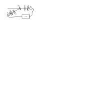
Figure 1: Brown-Twiss interferometer with polarization selection.

Presented setup is a Brown-Twiss interferometer with a quarter-wavelength plate and an analyzer in each arm. Both the plate and the analyzer in one arm could be rotated independently by an arbitrary angle. According to these angles there is a certain polarization of photons that corresponds to their lossless propagation through the arm. Let us assume that these polarization photon states are $a^{\dagger}(\theta,\phi)|vac\rangle$ for transmitted arm and $a^{\dagger}(\theta^{\prime},\phi^{\prime})|vac\rangle$ for reflected arm. In this case we would say that setup is ”tuned” to detect the biphotons in polarization state $|\Psi\rangle$ ( 2).

If we have the biphotons in state $|\Psi\rangle$ in the input of the setup the coincidence count rate would be non-zero. The most interesting question is what happen with coincidence count rate $R_{c}$ when the biphotons in the input of the setup that is tuned to state $|\Psi\rangle$ are in any other state $|\Psi^{\prime}\rangle$. The answer was obtained in masha:02 where was shown that $R_{c}\sim|\langle\Psi|\Psi^{\prime}\rangle|^{2}$. So this scheme is a realization of the projector of an input state on the fixed one. In particular if we have input state orthogonal to the one setup tuned there would not be any coincidences in the scheme. Thus the coincidence rate is zero if and only if the input state is orthogonal to the one setup tuned. The significance of this criterion would be shown at the next section.

The goal of our work was to demonstrate the ability to prepare any given polarization state $|\Psi\rangle$ and as a straightforward and practical example of given states, we chose the specific sequence that was presented in peres:00 . This sequence of 12 states can be used in an extended version of BB84 QKD protocol for qutrits. As it was shown one can construct 4 mutually unbiased bases with 3 orthogonal states in each from any three orthogonal states using discrete Fourier transformation. Using $\alpha=|2,0\rangle$, $\beta=|1,1\rangle$, $\gamma=|0,2\rangle$ as the first orthogonal basis we observed all 12 states shown in the table I.

Table 1: 12 states used in qutrit QKD protocol.

State	$|c_{1}|$	$|c_{2}|$	$|c_{3}|$	$\phi_{1}$	$\phi_{2}$	$\phi_{3}$
$|\alpha\rangle$	$1$	$0$	$0$	$0$	$0$	$0$
$|\beta\rangle$	$0$	$1$	$0$	$0$	$0$	$0$
$|\gamma\rangle$	$0$	$0$	$1$	$0$	$0$	$0$
$|\alpha^{\prime}\rangle$	$\frac{1}{\sqrt{3}}$	$\frac{1}{\sqrt{3}}$	$\frac{1}{\sqrt{3}}$	$0$	$0$	$0$
$|\beta^{\prime}\rangle$	$\frac{1}{\sqrt{3}}$	$\frac{1}{\sqrt{3}}$	$\frac{1}{\sqrt{3}}$	$0$	$120^{\circ}$	$-120^{\circ}$
$|\gamma^{\prime}\rangle$	$\frac{1}{\sqrt{3}}$	$\frac{1}{\sqrt{3}}$	$\frac{1}{\sqrt{3}}$	$0$	$-120^{\circ}$	$120^{\circ}$
$|\alpha^{\prime\prime}\rangle$	$\frac{1}{\sqrt{3}}$	$\frac{1}{\sqrt{3}}$	$\frac{1}{\sqrt{3}}$	$120^{\circ}$	$0$	$0$
$|\beta^{\prime\prime}\rangle$	$\frac{1}{\sqrt{3}}$	$\frac{1}{\sqrt{3}}$	$\frac{1}{\sqrt{3}}$	$0$	$120^{\circ}$	$0$
$|\gamma^{\prime\prime}\rangle$	$\frac{1}{\sqrt{3}}$	$\frac{1}{\sqrt{3}}$	$\frac{1}{\sqrt{3}}$	$0$	$0$	$120^{\circ}$
$|\alpha^{\prime\prime\prime}\rangle$	$\frac{1}{\sqrt{3}}$	$\frac{1}{\sqrt{3}}$	$\frac{1}{\sqrt{3}}$	$-120^{\circ}$	$0$	$0$
$|\beta^{\prime\prime\prime}\rangle$	$\frac{1}{\sqrt{3}}$	$\frac{1}{\sqrt{3}}$	$\frac{1}{\sqrt{3}}$	$0$	$-120^{\circ}$	$0$
$|\gamma^{\prime\prime\prime}\rangle$	$\frac{1}{\sqrt{3}}$	$\frac{1}{\sqrt{3}}$	$\frac{1}{\sqrt{3}}$	$0$	$0$	$-120^{\circ}$

where $\alpha$, $\beta$ and $\gamma$ with fixed number of primes are the orthogonal states belong to the same basis and a scalar product of any two states belong to different bases is equal to 1/3.

II EXPERIMENT

II.1 Experimental setup and method of measurement

Our setup consists of two parts: first one performed the preparation of the biphoton field in a desired state and second one provide the measurement of the obtained states.

The preparation part of our setup (Fig. 2) is built on the base of a balanced Mach-Zehnder interferometer (MZI) gleb:03 .

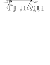
Figure 2: Experimental setup (preparation part).

The pump part consists of frequency doubled ”Coherent Mira 900” femtosecond laser, operated at central wavelength of 800 nm, 75 MHz repetition rate and with a pulse width of 100 fs, average pump power was 20 mW. The Glan-Tompson prism (GP), transmitting the horizontally polarized fraction of the UV pump and reflecting the vertically polarized fraction, serves as an input mirror of MZI. The reflected part, after passing the compensation BBO crystal and a half-wave plate (HWP2), pumps two consecutive 1 mm thick type-I BBO crystals whose optical axis are oriented perpendicularly with respect to each other. The biphotons from these crystals pass through a 10 mm quartz plate (QP1) that serves as a compensator, and the pump is reflected by an UV mirror. Then the biphotons arrive at a dichroic mirror (DM) that is designed to transmit them and to reflect the horizontally polarized component of the pump coming from the upper arm of MZI. A piezoelectric translator (PZT) was used to change the phase shift of the horizontal component of the pump with respect to the one propagating in the lower arm. The UV beam, reflected from DM serves as a pump for 1 mm thick type-II BBO crystal. Two 1 mm quartz plates (QP2) can be rotated along the optical axis to introduce a phase shift between horizontally and vertically polarized type-I biphotons, and a set of four 1 mm thick quartz plates (QP3) serves to compensate the group velocity delay between orthogonally polarized photons during their propagation in type II BBO crystal.

The measurement setup (Fig. 3) consists of a Brown-Twiss scheme with a non-polarizing 50/50 beamsplitter; each arm contains consecutively placed quarter- and half waveplates and an analyzer that was set to transmit the vertical polarization.

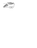
Figure 3: Experimental setup (measurement part).

This sequence of waveplates and analyzer is referred to as a polarization filter as soon as it extracts a single-photon polarization state defined by their orientation. Interference filters of 5 nm bandwidth, centered at 800 nm and pinholes are used for spectral and spatial modal selection of biphotons. We use EGG-SPCM-AQR-15 single photon counting modules as our detectors (D1 and D2). We should mention, that due to the low pump power, the stimulated processes in our setup are negligibly small and only pairs of photons have been generated. The measurement of the generated states is done using the tomography protocol that was developed for polarization qutrits leo:04 ; bogdan:03a . From experimental point of view we have to measure all fourth-order correlation moments in order to reconstruct coherence matrix

$K_{4}=$$\begin{pmatrix}A&D&E\\ D^{*}&C&F\\ E^{*}&F^{*}&B\end{pmatrix}$

which contains the following moments $\begin{array}[]{ccc}A=\langle a^{\dagger^{2}}a^{2}\rangle,&B=\langle b^{\dagger^{2}}b^{2}\rangle,&C=\langle a^{\dagger}b^{\dagger}ab\rangle,\\ D=\langle a^{\dagger^{2}}ab\rangle,&E=\langle a^{\dagger^{2}}b^{2}\rangle,&F=\langle a^{\dagger}b^{\dagger}b^{2}\rangle.\end{array}$

In the experiment one can measure directly only the diagonal elements of the coherency matrix. For example one measures B moment when there are only two vertical polarizers in the arms and no plates , adding quarter wavelength plate rotated at $45^{0}$ to one of the arms - C moment, adding quarter wavelength plates rotated at $45^{0}$ to each arm - A moment. In all other cases the coincidence rate would be proportional to linear combination of different moments. By choosing an appropriate combination containing as few number of moments as possible was proposed the following tomography protocol shown on the table 2.

Table 2: Tomography protocol. Each line contains orientation of the half ($\theta_{s,i}$) and quarter ($\chi_{s,i}$) wave plates in the measurement part of the experimental setup. Last column show the corresponding moment.

	Parameters of the experimental set-up				Moments to be measured
$\nu$	$\chi_{s}$	$\theta_{s}$	$\chi_{i}$	$\theta_{i}$
1.	0	$45^{\circ}$	0	$-45^{\circ}$	$A/4$
2.	0	$45^{\circ}$	0	0	$C/4$
3.	0	0	0	0	$B/4$
4.	$45^{\circ}$	0	0	0	$1/8(B+C+2\textrm{Im}F)$
5.	$45^{\circ}$	$22.5^{\circ}$	0	0	$1/8(B+C-2\textrm{Re}F)$
6.	$45^{\circ}$	$22.5^{\circ}$	0	$-45^{\circ}$	$1/8(A+C-2\textrm{Re}D)$
7.	$45^{\circ}$	0	0	$-45^{\circ}$	$1/8(A+C+2\textrm{Im}D)$
8.	$-45^{\circ}$	$11.25^{\circ}$	$-45^{\circ}$	$11.25^{\circ}$	$1/16(A+B-2\textrm{Im}E)$
9.	$45^{\circ}$	$22.5^{\circ}$	$-45^{\circ}$	$22.5^{\circ}$	$1/16(A+B-2\textrm{Re}E)$

As a result of the series of 9 measurements with different orientation of the plates in the arms of Brown-Twiss interferometer we can reconstruct the coherency matrix. Since we deal with a three-dimensional Hilbert space density matrix of measured state determined by 8 real numbers in general case when the state is mixed and by 6 real numbers in case of the pure state. In the experiment we have to provide one more measurement in order to find the normalization. Working with single mode biphoton polarization states we can completely describe them by means of the $K_{4}$. Since the coherence matrix carry full information about the state it can be used as well as the density matrix. But density matrix calculations are more usual, so we are going to use them. Polarization density matrix can be found from correlation moments by the formula dnk:97 ; bogdan:03a

$$\rho=\begin{pmatrix}2A&\sqrt{2}D&2E\\ \sqrt{2}D^{*}&C&\sqrt{2}F\\ 2E^{*}&\sqrt{2}F^{*}&2B\end{pmatrix}$$ (3)

Thus, after 9 measurements with the different orientations of the plates in the setup we have ehough information to reconstruct the density matrix of the polarization state. Moreover, this configuration of the measurement setup (fig. 3) allows us to verify the orthogonality of the states that belong to the same basis.

II.2 Compensation

In order to have the three terms in superposition (1) interfering, one must achieve their perfect overlap in frequency, momentum and time domains. From the experimental point of view this means that the biphoton wavepackets coming from the two type I crystals and from the type II crystal must be overlapped. The overlap in the frequency domain is achieved by the usage of 5nm bandwidth interference filters and the overlap in momentum is ensured by using pinholes that select one spatial mode of the biphoton field. But the overlap in time cannot be achieved easily when using a pulsed laser source, because it is necessary to compensate for all the group delays that biphoton wavepackets acquire during their propagation through the optical elements of the setup sergei:00 . It was found that in order to overlap type-I biphotons with type-II, the pump pulse from the lower arm must be delayed. In our case the value of the delay is  50 ps. This was achieved by inserting an additional 2 mm BBO crystal in the lower arm. The overlap between the states $|2,0\rangle$ and $|0,2\rangle$ was achieved by inserting a 10 mm quartz plate directly after the two type I BBO crystals. After overlapping the biphotons with these techniques, the average coincidence count rate that we observed was of about 1 Hz. The high visibility of interference patterns that we obtained was a criterion for a good compensation (see figures Fig. 4, Fig. 5, Fig. 6 in next section).

II.3 Calibration

In order to create a given qutrit state we needed to have independent control over four real parameters - two relative amplitudes and two relative phases.

Real amplitudes. In the experiment we used HWP1 to control the amplitude of the state $|1,1\rangle$, and HWP2 to control the relative amplitudes of the states $|2,0\rangle$ and $|0,2\rangle$. The calibration of these elements can be done by measuring moments related to $\rho_{11},\rho_{22},\rho_{33}$, defined in eq.  (4) in the tomography setup leo:04 . For our concrete experiment we had equal weights of each basis state in the superposition, so we had to set our waveplates in such a way that these moments fulfilled the condition: $\rho_{11}=\rho_{22}=\rho_{33}$. The values of the diagonal density matrix components were $\rho_{11}=0.355\pm 0.032,\rho_{22}=0.34\pm 0.046,\rho_{33}=0.305\pm 0.035$.

Phase $\phi_{13}$. The relative phase $\phi_{13}=\phi_{3}-\phi_{1}$ between states $|2,0\rangle$ and $|0,2\rangle$ can be controlled with the help of rotating quartz plates (QP2). The resulting state of biphoton field after these plates can be written as $|\Psi^{\prime}\rangle=|2,0\rangle+e^{i\phi_{13}}|0,2\rangle$. Varying the phase $\phi_{13}$ by rotating the quartz plates (QP), one can observe an interference pattern when the polarizers in Brown-Twiss scheme are set to transmit $+45^{\circ}$ and $-45^{\circ}$ polarized light olya:01 . This effect, known as ”space-time interference”, can be used to calibrate $\phi_{13}$, since we can assign value ”0” to the position of the minimum of interference pattern, and ”$\pi$” to the position of the maximum. An obtained typical dependence from this parameter is presented at (Fig. 4). A nonperiodic behavior is caused by a nonlinear dependence of an induced phase from the rotation angle. One can recalculate the dependence from the angle to dependence from the phase and the result is presented at (Fig. 5). This plot serves as a calibration curve for phase $\phi_{13}$.

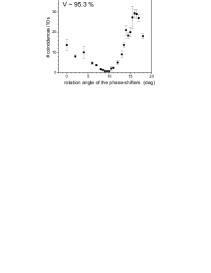
Figure 4: Space-time interference pattern for state $|\Psi^{\prime}\rangle=\frac{1}{\sqrt{2}}(|2,0\rangle+e^{i\phi_{13}}|0,2\rangle)$. Minimum corresponds to $\phi_{13}=\pi$, maximum corresponds to $\phi_{13}=0$.

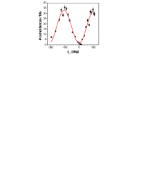
Figure 5: Space-time interference pattern for state $|\Psi^{\prime}\rangle=\frac{1}{\sqrt{2}}(|2,0\rangle+e^{i\phi_{13}}|0,2\rangle)$. Recalculated dependence on the phase $\phi_{12}$.

It is important to note that in order to ensure the resulting state being close to a pure state it is necessary to achieve as high visibility as possible in space-time interference experiment with type I biphotons and polarization interference of type II biphotons (Fig. 6). The obtained visibilities of approximately 95% were considered as a good result in order to proceed with a final stage of the experiment - the combination of states $|\Psi^{\prime}\rangle=|2,0\rangle+e^{i\phi_{13}}|0,2\rangle$ and $|1,1\rangle$ with a certain shift $\phi_{12}$ between them.

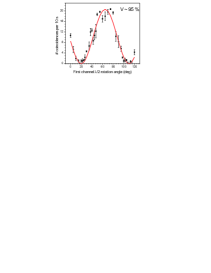
Figure 6: Polarization interference pattern from compensated type II biphotons.

Phase $\phi_{12}$: pump interference. The relation of the phase $\phi_{12}=\phi_{2}-\phi_{1}$ between the state $|\Psi^{\prime}\rangle$ and $|1,1\rangle$ to the voltage applied on PZT can be found by monitoring the pump interference pattern in M-Z interferometer. We found that the change of voltage by 1 V results in phase shift of $0.33rad$ .

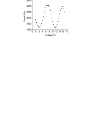
Figure 7: Pump interference pattern in Mach-Zehnder interferometer. The distance between two maxima (in Volts) corresponds to $\phi_{12}=\pi$.

Phase $\phi_{12}$: generation of superposition between $|2,0\rangle$ and $|1,1\rangle$ states. We also measured an interference pattern for a state $|\Psi^{\prime\prime}\rangle=\frac{1}{\sqrt{2}}(|2,0\rangle+exp(i\phi_{12})|1,1\rangle)$ varying the phase $\phi_{12}$. The polarization filters in Brown-Twiss scheme were set to measure moment $A$ of the tomography protocol. Moment $A$ exhibits no dependence on the phase $\phi_{12}$ for a given state. Therefore we inserted an additional polarization transformer - a zero-order quarter waveplate operated at 800 nm and oriented at $20^{\circ}$ with respect to the vertical direction. The unitary action of this waveplate is described by $3x3$ matrix that converts an input state $|\Psi^{\prime\prime}\rangle$ to another state that is sent to a measurement scheme quarks . For this certain waveplate, the state obtained after a transformer becomes

$$\Psi^{out}=\begin{pmatrix}(-0.25+0.32i)exp(i\phi_{12})-0.15\\ 0.41iexp(i\phi_{12})+0.25+0.32i\\ (0.25+0.32i)exp(i\phi_{12})+0.15-0.54i\end{pmatrix}$$ (4)

and now moment $A=c_{1}^{*}c_{1}$ shows a certain dependence on $\phi_{12}$. The experimentally obtained dependence (Fig. 8) can also be used to calibrate the phase. It is well known that a period of this interference pattern coincides with the the pump interference period. The theoretical visibility of the interference is equal to $64\%$, while the visibility obtained in the experiment is $53\%$. We attribute this difference to the misalignments of the setup.

We want to point out that in this experiment (for calibration purposes) we prepared a very specific superposition of basic states, interfering SPDC from type I and type II crystals, that was never reported in literature up to our knowledge.

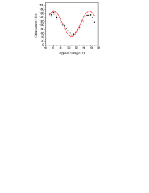
Figure 8: The interference pattern for state $|\Psi^{out}\rangle$. The distance between two maxima (in Volts) also corresponds to $\phi_{12}=\pi$.

II.4 Experimental procedure

In order to create a given qutrit state we needed to have independent control over four real parameters - two relative amplitudes and two relative phases. In the experiment we used HWP1 to control the amplitude of the state $|1,1\rangle$, and HWP2 to control the relative amplitudes of the states $|2,0\rangle$ and $|0,2\rangle$. The relative phase $\phi_{13}=\phi_{3}-\phi_{1}$ between the states $|2,0\rangle$ and $|0,2\rangle$ can be controlled with the help of rotating quartz plates (QP2). The relation of the phase $\phi_{12}=\phi_{2}-\phi_{1}$ between the state $|\Psi^{\prime}\rangle=|2,0\rangle+e^{i\phi_{13}}|0,2\rangle$ and $|1,1\rangle$ to the voltage applied to PZT can be found by monitoring the pump interference pattern in M-Z interferometer. We found that the change of voltage by 1 V resulted in the phase shift of $51.7^{\circ}$ and $\phi_{12}$ grew linearly with the applied voltage.

States that constitute the first basis are trivial (Table I). They can be produced with the help of a single crystal, corresponding to type I or type II interaction. State $|2,0\rangle$ is generated when first $\lambda/2$ (HWP1) angle corresponds to the maximal reflection of the pump beam into the lower arm of a Mach-Zehnder and the angle of the second half-lambda waveplate (HWP2) is equal to $0^{\circ}$. In order to generate state $|0,2\rangle$, the HWP2 must be rotated by $45^{\circ}$ degrees from $0^{\circ}$, and to generate state $|1,1\rangle$ the HWP1 is rotated such, that the whole pump goes into the upper arm of Mach-Zehnder. Therefore, in the following, we will consider only the generation of the rest nine states, i.e. those forming the other three bases. According to Table I, only the relative phases between the basic states are to be varied. This allows us to use the same settings of the HWP’s for the generation of nine states. It is also convenient to perform three sets of data acquisition - for the fixed $\phi_{13}$ values of $0$, $+120^{\circ}$ and $-120^{\circ}$, we change $\phi_{12}$ values in the range of, say, few periods and perform all tomographic measurements for each value of the phase $\phi_{12}$. Then we select the values of $\phi_{12}$ that correspond to the generation of the required state. For example, in order to generate the state $\beta^{\prime}$, we use $\phi_{13}=-120^{\circ}$ and $\phi_{12}=120^{\circ}$. The values of the moments at this point allow us to restore a raw density matrix of the generated state and compare it to the theoretical value.

The following procedure was used in order to verify the orthogonality of the states that form a certain basis. First we chose a set state to which we would tune our polarization filters. Then the values of the angles of quarter- and half- waveplates (Fig.  3) ($\chi_{1},\theta_{1},\chi_{2},\theta_{2}$) that assure the maximal projection of the polarization state of each photon on the $V$ direction can be calculated by mapping the set state on the Poincare sphere. Here, the lower index ”1” corresponds to the transmitted arm, and the index ”2” to the reflected arm of BS We chose states $|\alpha^{\prime}\rangle$, $|\alpha^{\prime\prime}\rangle$ and $|\alpha^{\prime\prime\prime}\rangle$ to be our set states for each basis. Then, by setting the phase $\phi_{13}$ fixed and by varying the phase $\phi_{12}$ we measured the number of coincidence counts that correspond to the certain fourth order moment of the field. According to the orthogonality criterion, the coincidence rate should fall to zero when the values of $\phi_{13}$ and $\phi_{12}$ correspond to the generation of the states orthogonal to the set ones.

II.5 Results and discussion

Let us consider the generation of the state $|\beta^{\prime\prime}\rangle$. In this case $\phi_{13}=0,\phi_{12}=120$. In Fig.  9 the measured values of the real and imaginary parts of the density matrix components $\rho_{21}$ and $\rho_{32}$ on phase $\phi_{12}$ are shown as function of the phase $\phi_{12}$. The number of accidental coincidences was negligibly small and was not subtracted in data processing.

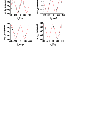
Figure 9: Imaginary and real values of non-diagonal density matrix components used to reconstruct state $|\beta^{\prime\prime}\rangle$. Theoretical dependence is plotted with a solid curve.

The phase $\phi_{13}=0$ remained constant during the tomography procedure. After obtaining the dependence of the moments $\rho_{21}$ and $\rho_{32}$ on phase $\phi_{12}$ we fitted our data with theoretical dependencies, using the least-square approximation method. The obtained values of all components were substituted in Eq. 4. The obtained density matrix for state $|\beta^{\prime\prime}\rangle$ is given below.

$$\rho_{\beta^{\prime\prime}}=\left(\begin{array}[]{ccc}0.355&-0.054-0.210i&0.315-0.010i\\ -0.054+0.210i&0.340&-0.106+0.262i\\ 0.315+0.010i&-0.106-0.262i&0.305\end{array}\right)$$ (5)

The eigenvalues of this matrix are $\lambda_{1}=0.877,\lambda_{2}=0.136,\lambda_{3}=-0.013$. A corresponding set of eigenvectors is $X=(0.587,-0.173+0.521i,0.594-0.071i);Y=(0.642,0.379-0.649i,0.048+0.143i);Z=(0.493,-0.287+0.224i,-0.769-0.178i)$. Although the density matrix (Eq. 5) is Hermitian and the condition $Tr(\rho)=1$ is satisfied, it doesn’t correspond to any physical state because of the negativity of one of the eigenvalues. We want to point out that a first main component $(\rho_{exp}^{1})_{ij}=X_{i}X_{j}^{\ast}$ of a considered density matrix, which has a weight $0.878$ is already close to the theoretical state vector $|\beta^{\prime\prime}\rangle$ and the corresponding fidelity is $F=Tr(\rho_{th}\rho_{exp}^{1})=0.9903$. The other two components correspond to the ”experimental noise” that is due mainly to misalignments of a setup and small volume of collected data. We have obtained similar eigenvalues for all other states and raw fidelity computed for the main density matrix component as described above have varied from 0.983 to 0.998. We also employed the maximum likelihood method of quantum state root estimation (MLE) bogdan:03a ; bogdan:03b to make a tomographically reconstructed matrix satisfy its physical properties, such as positivity. The results are presented in the following table (Table II). The level of statistical fluctuations in fidelity estimation was determined by the finite size of registered events $(\sim 500)$. All experimental fidelity values lie within the theoretical range of $5\%(F=0.9842)$ and $95\%(F=0.9991)$ quantiles quant ; bogdan:03a ; quant .

State	$F_{MLE}$	State	$F_{MLE}$	State	$F_{MLE}$
$|\alpha^{\prime}\rangle$	$0.9989$	$|\alpha^{\prime\prime}\rangle$	$0.9967$	$|\alpha^{\prime\prime\prime}\rangle$	$0.9883$
$|\beta^{\prime}\rangle$	$0.9967$	$|\beta^{\prime\prime}\rangle$	$0.9989$	$|\beta^{\prime\prime\prime}\rangle$	$0.9989$
$|\gamma^{\prime}\rangle$	$0.9883$	$|\gamma^{\prime\prime}\rangle$	$0.9883$	$|\gamma^{\prime\prime\prime}\rangle$	$0.9967$

Table 3: Fidelities estimated with Maximum Likelihood Method.

The obtained fidelity values show the high quality of the prepared states. The other test of the quality of states is the fulfillment of the orthogonality criterion for the states that belong to the same basis. For each set state we calculated the settings of waveplates in our measurement setup that ensured the maximal projection of each photon on the vertical polarization direction. In Fig. 10 we show the dependence of the coincidence rate for the following setting of waveplates $\chi_{1}=28.3^{\circ},\theta_{1}=-33.5^{\circ},\chi_{2}=-24^{\circ},\theta_{2}=-2^{\circ}$.

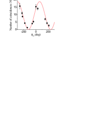
Figure 10: Dependence of number of coincidences on a phase $\phi_{12}$ for a given settings of polarization filters.

These values correspond to the set state $|\alpha^{\prime\prime\prime}\rangle$. As one can see, for the fixed value $\phi_{13}=0$ the coincidence rate is almost equal to zero, when phase $\phi_{12}=-120^{\circ}$. This corresponds to the generation of the state $|\beta^{\prime\prime\prime}\rangle$, which is orthogonal to $|\alpha^{\prime\prime\prime}\rangle$. The visibility of this pattern is equal to 93.2%. For the other bases, the obtained values of visibilities varied from 92% to 95%. With these values of visibility, the lowest value of coincidence rate corresponds to the accidental (Poissonian) coincidence level and therefore the obtained data verifies the orthogonality criterion.

Here we try to clarify how we understand the role of statistics in quantum state reconstruction. When we find that fidelity F = 0.990, then this result is sufficient without pointing out +/-0.XXX, because the obtained value shows only the degree of correspondence between the desirable result (to obtain fidelity as close to unity as possible) and the achieved precision of quantum state reconstruction. As usual, all works on quantum state tomography end up on this. At the same time we think that if we consider the question more thoroughly, it is necessary not only to point out the result, but also to try to answer the question about the principal precision that we can obtain in the experiment if we consider the finite (and not so large) volume of statistical data. Luckily we can also answer this question; it is overviewed in the paper bogdan:03a . On the basis of theory of statistical fluctuations of state vector estimation, that was developed in bogdan:03a , we obtained that the interval of the expected statistical fidelity fluctuations lies within 0.9842 (5% quantile) and 0.9991 (95% quantile).

The fact that all obtained fidelity values lie within that interval shows the correspondence of the experiment to the statistical theory. We also point out that due to the complexity of experiment, the volume of the data is not large (about 500 events in each of nine experiments). If we increase the volume of data, then, sooner or later, it will come to the point, when the correspondence of experiment to statistical theory will be violated. The experimentally achieved fidelity value would be lower then the theoretical due to the inevitable instrumental errors of experiment (see also bogdan:03a ) . In this case the quality of experiment can be estimated by the so called ”coherence volume” of data. If we exceed that volume, then the fidelity ”saturates” on the level which is somewhat less then unity. All further increase of the volume will not lead to the increase of fidelity since the precision of state reconstruction will be limited by the instrumental errors and instability of the experimental setup.

III Conclusions

We realized an interferometric method of preparing the three-level quantum optical systems, that relied on the polarization properties of single-mode two-photon light. The specific sequence of states was generated and measured with high fidelity values. The orthogonality of the states that form mutually unbiased bases was experimentally verified. As an advantage of this method we note that all control of the amplitudes and phases of each basic state in superposition (1) is done using linear optical elements, making it easy to switch from one state to another and providing the full control over the state (1) . The main disadvantage is that we cannot generate an entangled qutrits in this configuration. Our setup also allows one to prepare an arbitrary polarization qutrit state on demand.

- (1) H.Bechmann-Pasquinucci, A.Peres, Phys. Rev. Lett. 85, 3313 (2000).
- (2) D.Kaszlikowski, D.K.L Oi, M.Christandl, K.Chang, A.Ekert, L.C.Kwek and C.H.Oh, Phys. Rev.A. 67, 012310 (2003).
- (3) D.Bruss, C.Macchiavello, Phys. Rev. Lett. 88, 127901 (2002).
- (4) T.Durt, N.J.Cerf, N.Gisin and M.Zukowski, Phys. Rev.A. 67, 012311 (2003).
- (5) D.Collins, N.Gisin, N.Linden, S.Massar, S.Popescu, Phys. Rev. Lett. 88, 040404 (2002).
- (6) N.Langford, R.Dalton, M.Harvey, J.O’Brien, G.Pryde, A.Gilchrist, S.Bartlett, A.White, Phys. Rev. Lett. 93, 053601 (2004).
- (7) R.T.Thew, A.Acin, H.Zbinden, N.Gisin, Quantum Information and Computation, Vol.4, No.2, 93 (2004).
- (8) G.Molina-Terriza, A.Vaziri, J.Rehacek, Z.Hradil, A.Zeilinger, quant-ph/0401183.
- (9) A.Vaziri, J.-W.Pan, T.Jennewein, G.Weihs, and A.Zeilinger, Phys. Rev. Lett. 91, 227902 (2003).
- (10) J.C.Howell, A.Lamas-Linares, and D.Bouwmeester, Phys. Rev. Lett. 88, 030401 (2002).
- (11) A.Burlakov and M.Chekhova, JETP. 75, 432 (2002).
- (12) A.V.Burlakov and D.N.Klyshko, JETP Lett. 69, 839 (1999).
- (13) M.V.Chekhova, G.A.Maslennikov and A.A.Zhukov, JETP Letters. 76 (10), 696 (2002).
- (14) M.V.Chekhova, L.A.Krivitsky, S.P.Kulik, and G.A.Maslennikov, Phys. Rev.A. 70, 053801 (2004).
- (15) A.V.Burlakov, M.V.Chekhova, O.A.Karabutova, D.N.Klyshko, and S.P.Kulik, Phys. Rev. A. 60, R4209 (1999).
- (16) G.A.Maslennikov, M.V.Chekhova, S.P.Kulik and A.A.Zhukov, Journal of Optics B. 5, 530 2003.
- (17) L.A.Krivitsky, S.P.Kulik, A.N.Penin, and M.V.Chekhova, JETP 97, 846 (2003).
- (18) Yu.Bogdanov, M.Chekhova, S.Kulik, L.C.Kwek, A. Penin, M.K.Tey, C.H.Oh and A.Zhukov, Phys. Rev. A. 70, 042303 (2004).
- (19) D.N.Klyshko, JETP 84, 1065 (1997).
- (20) Y-H.Kim, M.Chekhova, S.Kulik, M.Rubin, and Y.Shih, Phys. Rev.A. 61, 051803(R) (2001).
- (21) Yu.I.Bogdanov, L.A.Krivitsky, S.P.Kulik, JETP Lett. 78, p.352 (2003).
- (22) The 5% and 95% quantiles cuts the left and right tail of distribution correspondingly.