Berry’s phase with quantized field driving: effects of inter-subsystem coupling

Abstract

The effect of inter-subsystem coupling on the Berry phase of a composite system as well as that of its subsystem is investigated in this paper. We analyze two coupled spin-$\frac{1}{2}$ with one driven by a quantized field as an example, the pure state geometric phase of the composite system as well as the mixed state geometric phase for the subsystem is calculated and discussed.

The concept of geometric phase was first introduced by Pancharatnam pancharatnam in his study on the interference of light in distinct states of polarization, and later was extended to its quantal counterpart by Berry berry84 , who shown that the state of a quantum system acquires a purely geometric feature in addition to the usual dynamical phase when it is varied slowly and eventually brought back to its initial form. The geometric phase has been extensively studied shapere89 ; thouless83 ; sun90 and generalized, for example to nonadiabatic evolution aharonov87 , mixed states uhlmann86 ; sjoqvist00a , and open systems carollo03 . All these studies were based on the semiclassical theory in the sense that the driving field itself has never been quantized. The effect due to the field quantization on the geometric phase was theoretically studied fuentes02 through a cavity QED model, where the cavity mode acted as the driving field, this work appears as the first study on the Berry phase with quantum field driven since no research devoted to this problem before. The other direction to which the Berry phase have been generalized is the Berry phase in composite systemsyi03 , this study was motivated by the application of geometric phase in quantum information processing as well as the theory of geometric phase itself.

From the application aspect, the implementation of quantum information by geometric means hold the merit of some built-in fault-tolerant features, because most systems for this purpose are composite, the study on the Berry phase of composite systems is highly required. From another aspect, since the geometric phase of entangled systems have attracted interest for its connection to the topology of the SO(3) rotation group milman03 and Bell’s theorem bertlmann03 , and the entanglement may be created only via interactions or joint measurements, how inter-subsystem coupling may affect the geometric phase of a composite system is of interest then.

In this Letter, we investigate the behavior of the geometric phase of a bipartite system with inter-subsystem coupling, one of the subsystems is driven by a quantized single mode of field, we examine the effect of inter-subsystem coupling on the pure state geometric phase of the composite system, as well as on the mixed state geometric phase of the subsystem. The composite system is designed to undergo an adiabatic and cyclic evolution while the subsystems remain on their non-transition state yi04 . An example of two coupled spin-$\frac{1}{2}$ systems with one driven by a quantized mode of field is presented to detail the representation. We calculate and analyze the effect of spin-spin coupling on the geometric phase of the composite system and those of the subsystem. The results presented in this Letter are twofold; it is an extension of the mixed state geometric phase to the case with quantized field driving, and it would generalize the study on the Berry phase induced by vacuum to composite systems with inter-subsystem couplings.

Consider a composite system consisting of two interacting spin-$\frac{1}{2}$ subsystems in the presence of a single quantized mode of field, in the rotating wave approximation (RWA) the Hamiltonian governing such a system reads

$$H=\frac{\omega}{2}(\sigma_{1}^{z}+\sigma_{2}^{z})+\nu a^{\dagger}a+\lambda(\sigma_{1}^{+}a+\sigma_{1}^{-}a^{\dagger})+J\sigma_{1}^{z}\sigma_{2}^{z},$$ (1)

where $\omega$ is the transition frequency between the eigenstates of the spin-$\frac{1}{2}$, which was assumed to be the same for the two subsystems, $\nu$ is the frequency of the field described in terms of the creation and annihilation operators $a^{\dagger}$ and $a$, respectively, $\lambda$ stands for the coupling constant between the field and the subsystem 1, and $J$ describes the coupling constant between the two spin-$\frac{1}{2}$. This model also can be understood to describe two two-level atoms with dipole-dipole interactions, one of the atoms interacting with a quantized cavity field, the difference is the interaction $J\sigma_{1}^{z}\sigma_{2}^{z}$ is not a typical dipole-dipole coupling, but rather a toy model describing a spin-spin interaction, nevertheless, the presentation in this Letter can be generalized to the cavity QED system with dipole-dipole coupling, in which the observation of such an effect is feasible with current technology.

To proceed further, let us first recount the methodfuentes02 for calculating the geometric phases in the full quantized regime. In the standard semiclassical theory, the field operators $a^{\dagger}$ and $a$ are replaced by the classical amplitude with rotation factors $e^{i\phi}$ and $e^{-i\phi}$, respectively. Changing $\phi$ slowly from $0$ to $2\pi$, the system would transport round a circuit in the parameter space and acquire a geometric phase in addition to the familiar dynamical phase factor. In the fully quantized context, the same procedure to generate an analogous phase change in the state of the field is needed, in practise the phase shift operator $U(\phi)=e^{-i\phi a^{\dagger}a}$ applied adiabatically to the Hamiltonian of the system may meet this need fuentes02 , this would give rise to the following eigenstate of the Hamiltonian Eq.(1) after the phase shift operator applied

$$|\psi_{1}\rangle = \cos\frac{\alpha}{2}e^{-in\phi}|e_{1},e_{2},n\rangle+\sin\frac{\alpha}{2}e^{-i(n+1)\phi}|g_{1},e_{2},n+1\rangle,$$

$$|\psi_{2}\rangle = -\sin\frac{\alpha}{2}e^{-in\phi}|e_{1},e_{2},n\rangle+\cos\frac{\alpha}{2}e^{-i(n+1)\phi}|g_{1},e_{2},n+1\rangle,$$

$$|\psi_{3}\rangle = \cos\frac{\beta}{2}e^{-in\phi}|e_{1},g_{2},n\rangle+\sin\frac{\beta}{2}e^{-i(n+1)\phi}|g_{1},g_{2},n+1\rangle,$$

$$|\psi_{4}\rangle = -\sin\frac{\beta}{2}e^{-in\phi}|e_{1},g_{2},n\rangle+\cos\frac{\beta}{2}e^{-i(n+1)\phi}|g_{1},g_{2},n+1\rangle,$$ (2)

with the corresponding eigenvalues, $E_{1,2}=\frac{\omega+(2n+1)\nu}{2}\pm\frac{2}{\sqrt{4\lambda^{2}(n+1)+(\omega+2J-\nu)^{2}}},$ $E_{3,4}=\frac{(2n+1)\nu-\omega}{2}\pm\frac{2}{\sqrt{4\lambda^{2}(n+1)+(\omega-2J-\nu)^{2}}},$ where $\alpha$ and $\beta$ are defined as

$$\cos\alpha = \frac{\omega+2J-\nu}{\sqrt{4\lambda^{2}(n+1)+(\omega+2J-\nu)^{2}}},$$

$$\cos\beta = \frac{\omega-2J-\nu}{\sqrt{4\lambda^{2}(n+1)+(\omega-2J-\nu)^{2}}},$$ (3)

and $|x_{1},y_{2},n\rangle\equiv|x_{1}\rangle\otimes|y_{2}\rangle\otimes|n\rangle(x,y=g,e)$ represents the basis of the composite system. In the same manner as that in the standard semiclassical theory, the Berry phase are calculated as $\gamma_{i}=i\int_{0}^{2\pi}\langle\psi_{i}|\frac{\partial}{\partial\phi}|\psi_{i}\rangle d\phi$, it yields

$$\gamma_{1} = 2n\pi+\pi(1-\cos\alpha),$$

$$\gamma_{2} = 2(n+1)\pi-\pi(1-\cos\alpha),$$

$$\gamma_{3} = 2n\pi+\pi(1-\cos\beta),$$

$$\gamma_{2} = 2(n+1)\pi-\pi(1-\cos\beta),$$ (4)

As shown in Ref.fuentes02 , the Berry phase are different from zero even for the driving field in the vacuum state ($n=0$), this indicates that the vacuum field may introduce a correction in the Berry phase. Furthermore, the Berry phases Eq. (4) would return to the semiclassical results when the driving field are prepared in a coherent state with large mean photon number, for more detail, we refer the reader to Ref.fuentes02 , here we mainly focus on the effects due to the inter-subsystem coupling. From Eq.(4), the effects due to the inter-subsystem coupling are obvious, all Berry phases tend to zero (or $2m\pi$, $m$ an integer) with the coupling constant $J\rightarrow\infty$ compared to $\lambda\sqrt{(n+1)}$, this fact makes the observation of the vacuum induced Berry phase in the composite system difficult, in other words, to observe the Berry phase induced by the vacuum field in the composite system, the system with small inter-subsystem coupling relative to the particle-field interaction is required. The composite system would acquire geometric phase $\pi$ or $-\pi$ when there is no inter-subsystem coupling and with resonant field-particle coupling ($\cos\alpha=\cos\beta=0$) , it nevertheless is not the case when the inter-subsystem couplings take place, the state would acquire a Berry phase different from $\pm\pi$ even if the particle-field coupling is on resonance ($\cos\alpha=-\cos\beta\neq 0$); this point can be understood as follows, the states of the subsystem 2 does not change during the interaction, hence the inter-subsystem coupling only results in a level shift to the subsystem 1, this leads to the effect different from the case without inter-subsystem couplings. Mathematically, the effect of the inter-subsystem coupling in Berry’s phase of the composite system may be simulated by the detuning $\delta=\omega-\nu$ in this model, however, when we extend this representation to a system with intra-variable coupling, the result will be changed, we will mention it again later on.

The physical meaning of the term $2\pi m$ ($m$, an integer) in Eq.(4) can be exhibited by the same scheme as in fuentes02 , i.e., by introducing the second mode of the field with creation and annihilation operators $b^{\dagger}$ and $b$ which initially does not interact with the two spin-$\frac{1}{2}$ nor the first mode of the field. The Hamiltonian describing such a system has the form

$$H_{0}^{2q}=\frac{\omega}{2}(\sigma_{1}^{z}+\sigma_{2}^{z})+\nu a^{\dagger}a+\nu b^{\dagger}b+\lambda(\sigma_{1}^{+}a+\sigma_{1}^{-}a^{\dagger})+J\sigma_{1}^{z}\sigma_{2}^{z},$$ (5)

where the second mode with the same frequency as the first one was assumed. The eigenstates of this Hamiltonian are

$$|\psi_{i}^{2q}\rangle=|\psi_{i}^{0}\rangle\otimes|n^{{}^{\prime}}\rangle,i=1,...,4$$ (6)

with $|\psi_{i}^{0}\rangle$ representing the eigenstates of the Hamiltonian Eq. (1). The state vector is a product state of the Fock state $|n^{{}^{\prime}}\rangle$ of the second mode of the field and the two spin-$\frac{1}{2}$ particles with one driven by the first field and with spin-spin couplings $J\sigma_{1}^{z}\sigma_{2}^{z}$. We proceeded to calculate the Berry phase of the system by changing adiabatically the Hamiltonian Eq.(5) via the unitary transformation

$$U(\theta,\phi)=exp(-i\phi J_{z})exp(-i\theta J_{y})$$ (7)

with $J_{z}=\frac{1}{2}(a^{\dagger}a-b^{\dagger}b)$ and $J_{y}=\frac{1}{2i}(a^{\dagger}b-ab^{\dagger})$, where $\theta$ and $\phi$ stand for slowly varying parameters. The transformed Hamiltonian $H^{2q}=U(\theta,\phi)H_{0}^{2q}U^{\dagger}(\theta,\phi)$ describes two coupling spin-$\frac{1}{2}$ interacting simultaneously with the two modes of the field. The four eigenstates Eq.(6) acquires geometric phase when $\phi$ is altered from $0$ to $2\pi$ adiabatically as

$$\gamma_{1}^{2q} = \pi\cos\theta(n-n^{{}^{\prime}}+\frac{1}{2})-\frac{\pi}{2}\cos\theta\cos\alpha,$$

$$\gamma_{2}^{2q} = \pi\cos\theta(n-n^{{}^{\prime}}+\frac{1}{2})+\frac{\pi}{2}\cos\theta\cos\alpha,$$

$$\gamma_{3}^{2q} = \pi\cos\theta(n-n^{{}^{\prime}}+\frac{1}{2})-\frac{\pi}{2}\cos\theta\cos\beta,$$

$$\gamma_{4}^{2q} = \pi\cos\theta(n-n^{{}^{\prime}}+\frac{1}{2})+\frac{\pi}{2}\cos\theta\cos\beta.$$ (8)

The contribution $\pi\cos\theta(n-n^{{}^{\prime}})$ may be understood as a phase acquired of a polarized field whose polarization slowly rotates and performs a closed loop in the poincaré’s sphere fuentes02 , hence it is inter-subsystem coupling independent. Terms $\frac{\pi}{2}\cos\theta(1\pm\cos\xi),\xi=\alpha,\beta$ are pure effects of field quantization which has no semiclassical correspondence, it makes nonzero contribution even if the particle-field coupling is on resonance, this is the very effect due to the spin-spin couplings.

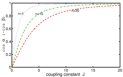
Figure 1: $\cos\alpha$ (or $\cos\beta$) as a function of spin-spin coupling constant $J$ (in units of $\lambda$, the spin-field coupling) with different photon number $n$.

Now we turn our attention to study the Berry phase of the subsystem. Uhlmann was the first to address the issue of mixed state geometric phase uhlmann86 , the analysis was generalized to mixed states undergoing unitary evolution sjoqvist00a and non-unitary evolutionyi03 from the viewpoint of interferometry. For unitary evolution, the mixed state geometric phase was defined as $\mbox{arg Tr}(U^{||}\rho)$ with $U^{||}$ representing the unitary parallel transport, whereas in the case of non-unitary evolution, it was defined as a weighted average over phase factors of the non-transition states. We will adopt the latter definition to study the properties of geometric phase for the subsystem. To start with, we write down the reduced density matrix corresponding to the instantaneous eigenstate $|\psi_{1}\rangle$ given by Eq.(2) for subsystem 1 in basis $\{|e_{1},n\rangle,|g_{1},n+1\rangle\}$ as

$$\rho_{1}=\left(\matrix{\cos^{2}\frac{\alpha}{2}&\cos\frac{\alpha}{2}\sin\frac{\alpha}{2}e^{i\phi}\cr\cos\frac{\alpha}{2}\sin\frac{\alpha}{2}e^{-i\phi}&\sin^{2}\frac{\alpha}{2}}\right),$$ (9)

it yields the mixed state geometric phase for subsystem 1

$$\gamma_{1}^{1}=\pi(1+\cos\alpha),$$ (10)

in the same way, the geometric phases for subsystem 1 pertaining to the other instantaneous eigenstates $|\psi_{2}\rangle,|\psi_{3}\rangle$ and $|\psi_{4}\rangle$ in Eq.(2) can be calculated as follows

$$\gamma_{2}^{1} = \pi(1-\cos\alpha),$$

$$\gamma_{3}^{1} = \pi(1+\cos\beta),$$

$$\gamma_{4}^{1} = \pi(1-\cos\beta),$$ (11)

These mixed state geometric phases are very similar to the geometric phase of the single spin-$\frac{1}{2}$ particle driving by the classical magnetic fieldberry84 , aside from an energy shift of $2J$ in $\cos\alpha$ and $\cos\beta$, the vacuum induced correction to the geometric phases of subsystem 1 also exist in this case, it can be seen from the definition of $\alpha$ and $\beta$ in Eq.(3). The dependence of $\cos\alpha$ and $\cos\beta$ on the photon number $n$ and the spin-spin coupling constant $J$ was represented in figure 1, where we choose $\omega=\nu$, i.e., the spin-field coupling is on resonance to plot the figure, $\cos\xi(\xi=\alpha,\beta)$ is the key quantity in this study, since all these phases are related to this quantity. From figure 1, we can see that the mixed state geometric phases Eq. ( 10,11) tend to zero (or 2$\pi$) with $J\rightarrow\infty$. The effect due to the field quantization is also clear from Eq.(8); they tend to $\frac{\pi}{2}\cos\theta$ with $J\rightarrow 0$ when the field-particle interaction is on resonance, and these phases tend to $\pi\cos\theta/0$ in the strong spin-spin coupling limit $J\rightarrow\infty$.

Finally, we discuss the problem of adiabaticity. In the standard semiclassical theory, the driving field has to change slowly to entail the system to undergo an adiabatic evolution, in the full quantum regime the adiabatic condition follows straightforwardly ($p,q=1,2,3,4$) from

$$|\frac{\langle\psi_{p}(t)|\frac{\partial}{\partial t}|\psi_{q}(t)\rangle}{E_{p}(t)-E_{q}(t)}|<<1,p\neq q,$$ (12)

and it is given that $\frac{\omega}{4}\lambda\sqrt{n+1}<<1$, with $\omega$ the precessing frequency ($\phi=\omega t$), which is independent of the spin-spin couplings, this indicates that the spin-spin couplings does not affect the adiabaticity of the composite system, which is quite different from the case with classical field driving yi042 . The extension of above analysis to the case of system with intra-variable coupling is straight forward. For example, consider an atom with electronic orbital and spin angular momentum $\vec{L}$ and $\vec{s}$, respectively, the spin-orbit coupling $\xi\vec{L}\cdot\vec{s}$ would play the role of the inter-subsystem coupling in the above discussion. The atom in this case may be treated as a composite system, and its geometric phase acquired when it transports round a loop in the parameter space strongly depends on the spin-orbit coupling, which is similar to the case with classical field driving.

To sum up, we have calculated the pure state Berry phases of the composite system and the mixed state geometric phases of its subsystems. The results show that the inter-subsystem coupling would diminish these phases and make the observation of the field quantization effect difficult. However, this is not the case when the driving field are of two modes, as Eq.(8) shows, the Berry phases due to the vacuum tend to $\frac{\pi}{2}(\cos\theta\pm\cos\theta)$ that would be a constant with a specific $\theta$. The adiabatic condition does not depend on the inter-subsystem coupling, this is quite different from the case with classical field driving.

XXY acknowledges financial support from EYTP of M.O.E, and NSF of China under project 10305002.

References

- (1) S. Pancharatnam, Proc. Indian Acad. Sci., Sect. A 44, 247(1956).
- (2) M. V. Berry, Proc. R. Soc. London Ser. A 392, 45 (1984).
- (3) Geometric phase in physics, Edited by A. Shapere and F. Wilczek ( World Scientific, Singapore, 1989).
- (4) D. Thouless, M. Kohmoto, M.P. Nightingale, and M. den Nijs, Phys. Rev. Lett. 49, 405 (1983); F. S. Ham, Phys. Rev. Lett. 58, 725 (1987); H. Mathur, Phys. Rev. Lett. 67,3325 (1991); H. Svensmark and P. Dimon, Phys. Rev. Lett. 73, 3387 (1994); M. Kitano and T. Yabuzaki, Phys. Lett. A 142, 321(1989).
- (5) C. P. Sun, Phys. Rev. D 41, 1318 (1990).
- (6) Y. Aharonov and J. Anandan, Phys. Rev. Lett. 58, 1593 (1987); J. Samuel and R. Bhandari, Phys. Rev. Lett. 60, 2339 (1988); N. Mukunda and R. Simon, Ann. Phys. (N.Y.) 205 (1993); Ann. Phys. (N.Y.) 269 (1993); A. K. Pati, Phys. Rev. A 52,2576(1995).
- (7) A. Uhlmann, Rep. Math. Phys. 24, 229 (1986).
- (8) E. Sjöqvist, A.K. Pati, A. Ekert, J.S. Anandan, M. Ericsson, D.K.L. Oi, and V. Vedral, Phys. Rev. Lett. 85, 2845 (2000); K. Singh, D.M. Tong, K. Basu, J.L. Chen, and J.F. Du, Phys. Rev. A 67, 032106 (2003). M. Ericsson, E. Sjöqvist, J. Brännlund, D.K.L. Oi, and A.K. Pati, Phys. Rev. A 67, 020101(R) (2003).
- (9) A. Carollo, I. Fuentes-Guridi, M. Franca Santos and V. Vedral, Phys. Rev. Lett. 90, 160402 (2003); R. S. Whitney and Y. Gefen, Phys. Rev. Lett. 90, 190402 (2003); G. De Chiara and G.M. Palma, Phys. Rev. Lett. 91, 090404 (2003).
- (10) I. Fuentes-Guridi, A. Carollo, S. Bose, and V. Vedral, Phys. Rev. Lett. 89, 220404 (2002); A. Carollo, I. Fuentes-Guridi, M. Franca Santos and V. Vedral, Phys. Rev. A 67, 063804(2003).
- (11) E. Sjöqvist, Phys. Rev. A 62, 022109(2000); X.X. Yi, L.C. Wang, and T.Y. Zheng, Phys. Rev. Lett. 90, 150406 (2004).
- (12) P. Milman and R. Mosseri, Phys. Rev. Lett. 90, 230403 (2003).
- (13) R.A. Bertlmann, K. Durstberger, Y. Hasegawa, and B.C. Hiesmayr, e-print: quant-ph/0309089.
- (14) X. X. Yi, and E. Sjöqvist, e-print: quant-ph/0403231 (Phys. Rev. A, to appear).
- (15) X. X. Yi, H. T. Cui, and H. S. Song (unpublished).