The time-reversal test for stochastic quantum dynamics

Abstract

The calculation of quantum dynamics is currently a central issue in theoretical physics, with diverse applications ranging from ultra-cold atomic Bose-Einstein condensates (BEC) to condensed matter, biology, and even astrophysics. Here we demonstrate a conceptually simple method of determining the regime of validity of stochastic simulations of unitary quantum dynamics by employing a time-reversal test. We apply this test to a simulation of the evolution of a quantum anharmonic oscillator with up to $6.022\times 10^{23}$ (Avogadro’s number) of particles. This system is realisable as a Bose-Einstein condensate in an optical lattice, for which the time-reversal procedure could be implemented experimentally.

The difficulty of real-time quantum dynamical calculations is caused by complexity. The computational resources required to directly represent the Hilbert space of a large quantum system are enormous. This problem led to Feynman’s proposal Feynman (1982) to develop quantum computer hardware for quantum dynamics. In the absence of such devices, digital computers must be employed for these calculations at present. Regardless of the hardware or software being utilised, there is a profound question of how one can check that results are calculated accurately. This is an especially difficult issue with the time-evolution of quantum many-body systems, which is one of the central challenges in theoretical physics. There are few exact solutions, yet results must be calculated systematically to within a known error in order to allow theoretical predictions to be tested experimentally.

Stimulated by the success of quantum Monte-Carlo methods in imaginary time Wilson (1974); Creutz (1980); Pollock and Ceperley (1984); Ceperley (1995), the method used here for real-time quantum dynamics relies on sampling a probabilistic phase-space representation. Related approaches include Wigner’s classical phase-space representation Wigner (1932), which was used to develop semi-classical approximations similar to those for quantum chaos calculations Tomsovic and Heller (1993), as well as other classical phase-space Husimi (1940); Glauber (1963); Cahill and Glauber (1969); Sudarshan (1963) representations. More recent phase-space methods for quantum simulations use a nonclassical phase-space together with a weight parameter analogous to those used in path-integrals Deuar and Drummond (2002). These methods allow quantum dynamical simulations from first principles without semiclassical approximations. However, the sampling error can become a limiting factor.

Fortunately, an important property of time-independent Hamiltonians is that evolution backward in time is equivalent to evolution forward in time under a Hamiltonian of the opposite sign. This suggests a simple yet powerful test that any unitary quantum dynamical simulation must pass. Beginning with a well-defined initial state, a simulation is evolved for a time period for which we are interested in the quantum dynamics. The Hamiltonian is then negated and the simulation evolved again for the same period. For reliable simulation all relevant initial observables should be recovered.

Phase-space methods utilising quasi-probability distributions lead one to sample an equivalent set of stochastic differential equations (SDEs) with random noise terms, and these techniques scale linearly with the number of modes Drummond and Gardiner (1980); Gardiner and Zoller (1999); Carusotto et al. (2001); Plimak et al. (2001). While such methods have been successful for many problems Drummond et al. (1993); Drummond and Hardman (1993), the sampling errors sometimes grow in time and eventually can become unmanageable. Similar issues are encountered in simulating classical chaos, where sensitive dependence on initial conditions leading to an exponential growth of errors Eckmann and Ruelle (1985) can be tested via time-reversal. However, the use of intrinsically random equations for time-reversible quantum evolution appears paradoxical. How can one have time-reversibility in a method which appears to introduce increasing entropy at each step? It is this question we focus on here, by showing that this type of time-evolution is in fact completely reversible due to the storage of information in quantum correlations.

All currently known phase-space methods can be represented in a unified manner by an expansion of the density operator as

$$\hat{\rho}=\int d\vec{\alpha}\,G(\vec{\alpha})\hat{\Lambda}(\vec{\alpha}),$$ (1)

where $G(\vec{\alpha})$ is a positive distribution function over the phase-space $\vec{\alpha}$, and $\hat{\Lambda}(\vec{\alpha})$ is an over-complete basis for the Hilbert space Corney and Drummond (2002). A variety of techniques can be realised by changing the basis set, the dynamical equations (which are equivalent under a “stochastic gauge” symmetry Drummond and Deuar (2003)), and the numerical integration algorithm. We illustrate the time-reversal test for the particular case of a stochastic gauge simulation Deuar and Drummond (2002); Drummond and Deuar (2003). For this method the phase-space is $\vec{\alpha}=(\underline{\alpha},\underline{\beta},\Omega)$, which is a $2M+1$ complex dimensional vector containing phase-space variables $\alpha_{k}$ and $\beta_{k}$ (where $\underline{\alpha}=\{\alpha_{1},\dots,\alpha_{k},\dots,\alpha_{M}\}$, etc.) for each of $M$ bosonic modes, together with an additional variable $\Omega$ termed the weight. The operator basis is

$$\hat{\Lambda}(\vec{\alpha})=\Omega\bigotimes_{k}\frac{|\alpha_{k}\rangle\langle\beta_{k}^{*}|}{\langle\beta_{k}^{*}|\alpha_{k}\rangle}\,\,,$$ (2)

where the coherent state $\left|\alpha_{k}\right\rangle$ is an eigenstate of the boson annihilation operator $\hat{a}_{k}$ for the $k$th mode, with a mean boson number $\bar{n}_{k}=\langle\hat{a}_{k}^{{\dagger}}\hat{a}_{k}\rangle\,\,=|\alpha_{k}|^{2}$.

For two-body interactions the master equation for time evolution of the density operator can be shown to be equivalent to a Fokker-Planck equation for the evolution of the quasi-probability gauge distribution $G(\vec{\alpha})$ with basis (2). This in turn is equivalent to a set of SDEs. The moments of the gauge distribution function are then equivalent to dynamical quantum averages of products of bosonic creation and annihilation operators. For a single mode this equivalence can be expressed (from now on we omit the mode label $k$) as

$$\langle\left(\hat{a}^{\dagger}\right)^{m}\hat{a}^{n}\rangle_{\mathrm{QM}}=\frac{\langle\Omega\beta^{m}\alpha^{n}+(\Omega\alpha^{m}\beta^{n})^{*}\rangle_{\mathrm{stoch}}}{\langle\Omega+\Omega^{*}\rangle_{\mathrm{stoch}}},$$ (3)

where $\langle\rangle_{\mathrm{QM}}$ indicates a quantum mechanical average, and $\langle\rangle_{\mathrm{stoch}}$ is a stochastic average.

In this paper we consider the anharmonic oscillator Hamiltonian

$$\hat{H}=\frac{\hbar\kappa}{2}\hat{a}^{\dagger 2}\hat{a}^{2},$$ (4)

which describes both the Kerr effect in nonlinear optics, and a single mode Bose-Einstein condensate (BEC). It is perhaps the simplest model of a many-body quantum system, and, as it is analytically solvable, it provides an excellent testing ground for simulation methods.

An important quantum feature of this Hamiltonian is that given an initial coherent state $\hat{\rho}(0)=\left|\alpha\right\rangle\left\langle\alpha\right|$, the dynamics display a series of collapses and revivals. From the analytic solution it is known that the quantum averages of the quadrature variables $\hat{X}=(\hat{a}+\hat{a}^{\dagger})/2$ and $\hat{Y}=(\hat{a}-\hat{a}^{\dagger})/2i$ undergo oscillations that eventually damp out to zero. However, after a certain time the oscillations revive, and the initial state is recovered. Defining the dimensionless time variable $\tau=\sqrt{\bar{n}}\kappa t/2\pi$, where $\bar{n}=|\alpha|^{2}$ is the mean particle number, the relevant time scales are the oscillation period $\tau_{\mathrm{osc}}\sim O(1/\sqrt{\bar{n}})$, the collapse time $\tau_{\mathrm{coll}}\sim O(1)$, and the revival time $\tau_{\mathrm{rev}}=\sqrt{\bar{n}}$. For large $\bar{n}$ the revival time is many times the collapse time, which in turn is much longer than the natural oscillation period. This revival is a uniquely quantum feature that does not occur in classical dynamics.

While single mode Hamiltonians are often not a good description of real systems, the anharmonic oscillator can be a good approximation for a Bose-Einstein condensate (BEC) in an optical lattice in the Mott insulator regime Greiner et al. (2002a). A sudden increase in the lattice depth from the superfluid regime can create coherent superpositions of atoms at each site which can be approximated by a coherent state. Indeed, such collapses and revivals have been observed with a BEC in a deep lattice Greiner et al. (2002b).

With a suitable choice of stochastic gauge representation Deuar and Drummond (2002) it was found to be possible to simulate past the collapse time with small statistical error using a modest number ($\sim 10^{4}$) of stochastic trajectories Drummond and Deuar (2003). Here we check this calculation with the time-reversal test to demonstrate that the full quantum nature of the dynamics is preserved, even when the mean quadrature amplitudes are near zero.

One finds Drummond and Deuar (2003) that the Ito SDEs corresponding to the anharmonic oscillator Hamiltonian (4) are

$$\dot{\alpha} = i\alpha\left[-\kappa n_{x}+\xi_{g,1}\right],$$ (5)

$$\dot{\beta} = i\beta\left[\kappa n_{x}+\xi_{g,2}^{*}\right],$$ (6)

$$\dot{\Omega} = -\Omega n_{y}e^{-g}\sqrt{i\kappa}\left[\xi_{1}-i\xi_{2}\right],$$ (7)

where $n=n_{x}+in_{y}=\alpha\beta$ is a complex variable corresponding to the particle number. Here $\xi_{g,j}$ are defined as transformations of the fundamental noise terms $\xi_{j}$ through the introduction of an arbitrary stochastic diffusion gauge $g$, chosen for efficiency:

$$\xi_{g,j}(t)=\sqrt{i\kappa}\left[\xi_{j}\cosh g+i\xi_{3-j}\sinh g\right].$$ (8)

For numerical integration with time steps $dt$, the $\xi_{j}$ can be implemented by independent real Gaussian noises of variance $1/dt$ and mean zero at each time step. The drift gauge used to obtain the deterministic parts of the equations from the Hamiltonian has been described previously Drummond and Deuar (2003). It is convenient to transform these equations to logarithmic variables, and to use the Stratonovich calculus for integration Gardiner and Zoller (1999). To obtain the time-reversed SDEs we simply replace $\kappa$ with $-\kappa$ in the above equations, and generate new, uncorrelated noises.

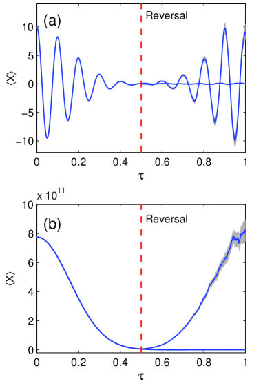
Figure 1: (Color online) Time-reversal test for a stochastic gauge simulation of the $X$-quadrature of the anharmonic oscillator. (a) An initial coherent state with mean boson number $\bar{n}=100$ and $10^{5}$ stochastic trajectories. (b) An initial coherent state with $\bar{n}=6.022\times 10^{23}$ and $10^{7}$ stochastic trajectories, with the calculation performed in the rotating frame. The solid lines are the simulation result for $\langle\hat{X}\rangle$, with the statistical error bars (representing one standard deviation) shown by the grey shading. For both cases the time-reversal was implemented at $\tau_{R}=0.5$ by negating the sign of the Hamiltonian and the initial state is recovered to within statistical error at $\tau=2\tau_{R}$. The forward time evolution to $2\tau_{R}$ demonstrating the collapse to $\langle\hat{X}\rangle$ = 0 is also shown in both (a) and (b).

Figure 1 illustrates the time-reversal test for the calculation of the dynamics of the quantum average of the $X$-quadrature. The initial coherent state has $\bar{n}=\langle\hat{a}^{{\dagger}}\hat{a}\rangle=100$, and each stochastic trajectory was evolved forward in time until $\tau_{R}=0.5$, using a constant diffusion gauge of $g=1.6$. The Hamiltonian was then negated and the system evolved again for the same period. We observe a reversal in the $X$-quadrature dynamics back to its initial value to within statistical error, even though each stochastic trajectory has evolved with uncorrelated noises at every point in the time-evolution. Of course, there are random features in each trajectory that are not time-reversed, but these change the distribution in a way that does not affect observables. This remarkable property is due to the overcompleteness of the quantum mechanical basis of coherent states, which permits the same physical state to be represented in more than one way in terms of coherent states.

While certainly not small, a one-hundred dimensional Hilbert space is accessible with current computers. We have therefore repeated this calculation for a much larger mean boson number equal to Avogadro’s number $\bar{n}=6.022\times 10^{23}$ — a truly macroscopic number of particles. This requires us to make use of more sophisticated gauge methods, with

$$g(\tau,\vec{\alpha})=\frac{1}{6}\log\left\{\frac{8\pi}{\sqrt{\bar{n}}}|n(\tau)|^{2}[2\tau_{R}-\tau]+\left[1+4n_{y}^{2}(\tau)\right]^{3/2}\right\}.$$ (9)

Further details on choices of gauges will be published elsewhere, also see Deuar (2004).

Here the total Hilbert space dimension is astronomically large, and well beyond the capacity of any known or planned digital computer. The dynamical evolution obtained from the analytic result is a Gaussian amplitude decay, quite different to the usual exponential decay of a damped system. While the amplitude decay appears to correspond to information loss, in fact there is information stored in quantum correlations, which can be recovered through time-reversal.

In this situation the physical collapse time is very short indeed — orders of magnitude less than the revival time — and there are many oscillations of the $X$-quadrature. We therefore perform the calculation in a rotating frame, and the envelope of the oscillations is plotted in Fig. 1(b). The time reversal is implemented at $\tau_{R}=0.5$, and again we can see the revival of the initial state. While this situation is somewhat idealised, it demonstrates a fully quantum calculation for a macroscopic particle number.

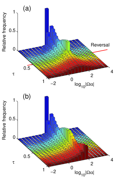
Figure 2: (Color online) A representation of the broadening of the gauge distribution function for $\bar{n}=100$. The plots are histograms of the quantity $\log_{10}|\alpha\Omega|$ for the stochastic trajectories at a number of points in time. (a) The time-reversed case with the Hamiltonian negated at $\tau_{R}=0.5$ and further evolved to $\tau=2\tau_{R}$. (b) The forward time evolution to $\tau=2\tau_{R}$. The initial distribution at $\tau=0$ for both graphs is a delta function, however it broadens with time to span several orders of magnitude at $\tau=2\tau_{R}$, despite being another representation of the initial quantum state in (a). Note that the logarithm of $|\alpha\Omega|$ is binned.

The important result to note is that in both cases the time-reversed quadrature mean agrees with the initial value to within the sampling error-bars. The error-bars can be reduced by including more trajectories in the calculation.

For these calculations the time-reversal test illustrates a powerful yet counterintuitive feature of stochastic simulations — they can be useful for simulating unitary (reversible) quantum dynamics, despite the irreversible nature of stochastic processes. The examples demonstrate a stochastic simulation of a quantum revival, a uniquely unitary feature. As discussed previously, the quadrature variables will display a true revival to their initial values at $\tau_{\mathrm{rev}}=\sqrt{\bar{n}}$. By time-reversing the calculation after the initial collapse we induce the revival early. However, the stochastic trajectories themselves continue to diffuse under time-reversal — they do not simply retrace their forward-time path. Hence, although it seems natural to associate irreversible stochastic process with irreversible quantum dynamics (such as those of an open quantum system), clearly this intuition is unnecessarily restrictive.

The calculation can equivalently be discussed in terms of the distribution function. During both the forwards and backwards time dynamics the gauge distribution $G(\vec{\alpha})$ evolves according to a Fokker-Planck equation with positive-definite diffusion and therefore can only broaden in phase space. This is clearly illustrated in Fig. 2. The gauge distribution function that is recovered after the reversal in Fig. 2(a) is not the same as the initial condition, but is still equivalent to the original density operator. This final distribution is less compact than the original, but nonetheless will have identical moments corresponding to the normally-ordered operator averages of the initial state. For this example we have sampled a gauge distribution $G(\vec{\alpha})$ at $2\tau_{R}$ that is equivalent to the initially chosen delta function $G(\vec{\alpha})=\delta^{2}(\alpha-\beta^{*})\delta^{2}(\Omega-1)\delta^{2}(\alpha-\sqrt{\bar{n}})$. This is precisely what must happen at the true revival time $\tau=\sqrt{\bar{n}}$. Fig. 2(b) shows the behaviour of the distribution function for the forward time evolution for comparison.

Although the calculations are presented as a method of testing quantum simulations, an early revival could be observed experimentally with a BEC in an optical lattice using the phenomenon of a Feshbach resonance Cornish et al. (2000); Weber et al. (2003). This allows the tuning of both the magnitude and sign of the interaction strength in atomic Bose gases, represented by our parameter $\kappa$, using an applied magnetic field. As the setup of Greiner et al. Greiner et al. (2002b) uses only optical potentials for the observation of revivals, an early revival experiment could be performed simply with the addition of a precisely-controlled homogeneous magnetic field.

We note that while the calculation presented is for a quantum phase space method, the time-reversal test is applicable to any quantum simulation technique. It is not a sufficient test in itself, since a time-reversible simulation could have other systematic errors. However, it has the great advantage that time-reversibility is an exact property of unitary quantum dynamics even when no other exact properties are known. We believe that the current status of calculating the dynamics of quantum many-body systems is similar to the situation in the early days of studying classically chaotic systems on a computer. By definition such systems display sensitive dependence on initial conditions, and so it is difficult to estimate the errors in the calculated dynamics Eckmann and Ruelle (1985). It was partly due to time-reversal tests that such calculations became convincing.

In summary, we have presented a simple yet powerful test for unitary quantum dynamics, and demonstrated its use to verify the results of a stochastic numerical simulation in a macroscopically large Hilbert space. Such tests are crucial for these demanding calculations. An increasing variety of quantum dynamical techniques are now becoming available, and it is important to have reliable tests of their accuracy — especially since no analytic solutions exist in many cases of interest.

We gratefully acknowledge research support from the Australian Research Council.

References

- Feynman (1982) R. P. Feynman, Int. J. Theor. Phys. 21, 467 (1982).
- Wilson (1974) K. G. Wilson, Phys. Rev. D 10, 2445 (1974).
- Creutz (1980) M. Creutz, Phys. Rev. D 21, 2308 (1980).
- Pollock and Ceperley (1984) E. L. Pollock and D. M. Ceperley, Phys. Rev. B 30, 2555 (1984).
- Ceperley (1995) D. M. Ceperley, Rev. Mod. Phys. 67, 279 (1995).
- Wigner (1932) E. Wigner, Phys. Rev. 40, 749 (1932).
- Tomsovic and Heller (1993) S. Tomsovic and E. J. Heller, Phys. Rev. E 47, 282 (1993).
- Husimi (1940) K. Husimi, Proc. Phys. Math. Soc. Japan 22, 264 (1940).
- Glauber (1963) R. J. Glauber, Phys. Rev. 131, 2766 (1963).
- Cahill and Glauber (1969) K. E. Cahill and R. J. Glauber, Phys. Rev. 177, 1882 (1969).
- Sudarshan (1963) E. C. G. Sudarshan, Phys. Rev. Lett. 10, 277 (1963).
- Deuar and Drummond (2002) P. Deuar and P. D. Drummond, Phys. Rev. A 66, 033812 (2002).
- Drummond and Gardiner (1980) P. D. Drummond and C. W. Gardiner, J. Phys. A: Math. Gen. 17, 2353 (1980).
- Gardiner and Zoller (1999) C. W. Gardiner and P. Zoller, Quantum Noise (Springer, Berlin, 1999), 2nd ed.
- Carusotto et al. (2001) I. Carusotto, Y. Castin, and J. Dalibard, Phys. Rev. A 63, 023606 (2001).
- Plimak et al. (2001) L. I. Plimak, M. K. Olsen, and M. J. Collett, Phys. Rev. A 64, 025801 (2001).
- Drummond et al. (1993) P. D. Drummond, R. M. Shelby, S. R. Friberg, and Y. Yamamoto, Nature 365, 307 (1993).
- Drummond and Hardman (1993) P. D. Drummond and A. D. Hardman, Europhys. Lett. 21, 279 (1993).
- Eckmann and Ruelle (1985) J. P. Eckmann and D. Ruelle, Rev. Mod. Phys. 57, 617 (1985).
- Corney and Drummond (2002) J. F. Corney and P. D. Drummond, Phys. Rev. A 68, 063822 (2002).
- Drummond and Deuar (2003) P. D. Drummond and P. Deuar, J. Opt. B: Quantum Semiclass. Opt 5, S281 (2003).
- Greiner et al. (2002a) M. Greiner, O. Mandel, T. Esslinger, T. W. Hänsch, and I. Bloch, Nature 415, 39 (2002a).
- Greiner et al. (2002b) M. Greiner, O. Mandel, T. W. Hänsch, and I. Bloch, Nature 419, 51 (2002b).
- Deuar (2004) P. Deuar, Ph.D. thesis, University of Queensland (2004).
- Cornish et al. (2000) S. L. Cornish, N. R. Claussen, J. L. Roberts, E. A. Cornell, and C. E. Wieman, Phys. Rev. Lett. 85, 1795 (2000).
- Weber et al. (2003) T. Weber, J. Herbig, M. Mark, H.-C. Nägerl, and R. Grimm, Science 299, 232 (2003).