Quantum Fidelity Decay of Quasi-Integrable Systems

Abstract

We show, via numerical simulations, that the fidelity decay behavior of quasi-integrable systems is strongly dependent on the location of the initial coherent state with respect to the underlying classical phase space. In parallel to classical fidelity, the quantum fidelity generally exhibits Gaussian decay when the perturbation affects the frequency of periodic phase space orbits and power-law decay when the perturbation changes the shape of the orbits. For both behaviors the decay rate also depends on initial state location. The spectrum of the initial states in the eigenbasis of the system reflects the different fidelity decay behaviors. In addition, states with initial Gaussian decay exhibit a stage of exponential decay for strong perturbations. This elicits a surprising phenomenon: a strong perturbation can induce a higher fidelity than a weak perturbation of the same type.

Manifestations of chaos and complexity in the quantum realm have been widely explored in connection with the correspondence principle between classical and quantum mechanics H1 . An example is a system’s response to small perturbations of its Hamiltonian. Peres Peres1 ; Peres2 conjectured that this response serves as an indicator of chaos applicable to both the classical and quantum realms. That is, in both realms the behavior of fidelity between a state evolved under perturbed and unperturbed dynamics depends on whether or not the dynamics is chaotic.

Peres’ conjecture found an experimental venue in nuclear magnetic resonance (NMR) polarization echoes. In these experiments the initial state of the system is evolved forward under its internal dipolar Hamiltonian and then inverted by a sequence of radio-frequency pulses RF . The inverted Hamiltonian, however, will be not be an exact reversal of the internal Hamiltonian due to pulse imperfections and interactions with the environment. These perturbations reduce the subsequent echo amplitude which is the measure of fidelity.

The polarization echo as a means of studying dynamical irreversibility was applied in Ref. LUP , where it was noted that the echo decay behavior as a function of time can be exponential or Gaussian, depending on the molecule under investigation. The connection between these results and the exponential fidelity decay predicted for systems exhibiting quantum chaos Peres2 was made in Ref. UPL .

Encouraged by these experimental investigations, Jalabert and Pastawski Jala applied semi-classical analysis to the evolution of what they termed the Loschmidt echo, or fidelity decay. Their analysis showed that for chaotic systems, when the perturbation is strong enough such that perturbation theory fails, the fidelity decay is comprised of two exponentially decaying terms. The first of these terms is dominant for small errors and can be described by the Fermi golden rule J1 ; C1 . The second term is dominant for strong errors, independent of perturbation strength, and decays at a rate given by the analogous classical system’s Lyapunov exponent.

The identification of a classically chaotic signature in quantum systems has led to detailed studies of fidelity decay behavior. For quantum systems that are analogs of classically chaotic systems, a number of regimes have been identified based on perturbation strength. For weak perturbations, such that perturbation theory is valid, the fidelity decay is Gaussian Peres1 ; J1 ; V1 . For stronger perturbations, in the Fermi golden rule regime, the fidelity decays exponentially with a rate determined by the perturbation Hamiltonian and perturbation strength Jala ; J1 ; P1 ; J2 ; Jo . In many systems the rate of the exponential increases as the square of the perturbation strength J1 (see W1 for an exceptional case) until saturating at the underlying classical systems’ Lyapunov exponent Jala ; C1 or at the bandwidth of the Hamiltonian J1 . The crossover between the various regimes Cerr1 ; Cerr2 ; Wang2 and the fidelity saturation level YSW1 ; W2 have also been explored. Quantum fidelity decay simulations have also been carried out in weakly chaotic systems Wang1 , and at the edge of quantum chaos YSW2 .

Relationships between fidelity decay behavior and other quantum phenomena are also found in the literature. These include the Fourier transform relation between fidelity decay and the local density of states J1 ; W3 , issues of classical-quantum correspondence Ben1 , reversibility Cohen1 , and decoherence C2 . We also note that fidelity decay studies can be carried out on a quantum computer Jo ; Poulin , and that the fidelity has been experimentally determined for a three-qubit quantum baker’s map on a NMR quantum information processor baker .

Studies of fidelity decay in quantum systems have spurred interest in the fidelity decay of classical systems Eck . For chaotic classical systems it has been shown that the asymptotic fidelity decay can be either exponential or power-law, analogous to the asymptotic decay of correlation functions BCV2 . Faster than Lyapunov exponential decays have also been identified VP .

The fidelity decay behavior of quantum analogs of non-chaotic or quasi-integrable classical systems has received less attention P1 ; P3 ; L1 then its chaotic counterpart and has been the subject of some controversy P2 ; J3 . Using semi-classical arguments, Prosen P1 ; P2 demonstrated the counter-intuitive result that quantum fidelity decay of regular, non-chaotic, evolution is Gaussian, faster than the exponential decay of chaotic systems. This was challenged by further semi-classical arguments J3 which indicated a power-law decay. A proposed resolution P3 differentiates between individual minimum uncertainty states, which generally exhibit a Gaussian decay, and averages over many such states, which may be biased by specific states exhibiting power-law fidelity decay behavior.

In this work, we explore what causes a quantum state undergoing regular quantum evolution to exhibit Gaussian or power-law fidelity decay behavior. We present numerical results demonstrating that the behavior depends on the reaction of the underlying classical phase space to the applied perturbation. Building off classical fidelity decay results Ben2 , we chart the regions of phase space containing states with initial Gaussian or power-law decay. Within the two regions we show that the exact rate of the Gaussian or power-law decay is also a function of the coherent state position. In addition, a connection is presented between fidelity decay behavior and the spectrum of the initial state in the eigenbasis of the system. Finally, we probe the dependence of the initial decay behavior on perturbation strength, Hilbert space dimension, and note that, for strong perturbations, there exists a transitional exponential fidelity decay behavior after initial Gaussian decay and before fidelity saturation.

Perturbing classical Hamiltonian evolution can affect phase space orbits in two general ways: the perturbation may distort the shape of the orbit or change the frequency of the orbit. Benenti, Casati, and Veble (BCV) Ben2 proposed that in the limit of weak perturbations the classical fidelity decay behavior is solely determined by the dominant perturbation effect on the phase space orbits. If the dominant effect on a specific orbit is to change its frequency, initial wave packets centered in the region exhibit Gaussian decay (assuming Gaussian wave packets). This is what would be expected from the fidelity of two Gaussian wave packets moving in antiparallel directions, or at different speeds, along a specific path. If, however, the effect of the perturbation is to change the shape of the KAM torus, states centered in the region will exhibit power-law fidelity decay. BCV note that they expect similar results in the quantum realm.

Here, we provide numerical evidence that the correspondence between the perturbation’s effect on phase space and fidelity decay behavior extends to quantum systems. Specifically, we show that quantum fidelity decay behavior depends on whether an initial coherent state is centered on a phase space orbit whose frequency is changed due to the perturbation, in which case the decay will be Gaussian, or an orbit whose shape is distorted by the perturbation, in which case the decay will be power-law. Fidelity decay simulations under quantum kicked rotor evolution support a suspicion of Ref. Ben2 , that quantum states are more prone to Gaussian decay due to the quantization of the phase space tori.

The quantum fidelity decay of an initial state $|\psi_{i}\rangle$ is given by

$$F(t)=|\langle\psi_{i}|U^{-t}U_{p}^{t}|\psi_{i}\rangle|^{2}$$ (1)

where $U$ is the unperturbed evolution, $U_{p}=Ue^{-i\delta V}$ is the perturbed evolution, $\delta$ is the perturbation strength, and $V$ is the perturbation Hamiltonian. Our numerical work is centered around kicked maps with kick strength $k$ determining whether the evolution is chaotic or regular. For the perturbed evolution we employ the same map with a slightly different kick strength. Thus, the unperturbed operator is $U=U(k)$, and the perturbed operator is $U_{p}=U(k+\delta_{k})$, with perturbation strength $\delta_{k}$.

We begin our study of fidelity decay with the quantum kicked top (QKT) H2 , a system used in many previous studies of quantum chaos in general H1 and fidelity decay in particular Peres2 ; J1 ; P1 ; Jo ; P3 ; J3 . The classical kicked top describes dynamics on the surface of a sphere

$$x_{t+1} = z_{t}$$

$$y_{t+1} = x_{t}\sin(k_{T}z)+y_{t}\cos(k_{T}z)$$

$$z_{t+1} = -x_{t}\cos(k_{T}z)+y_{t}\sin(k_{T}z),$$ (2)

where $k_{T}$ is the kick strength. We choose a kick strength of $k_{T}=1.1$ corresponding to quasi-integrable dynamics. The $\phi-\theta$ phase space of the classical kicked top is shown in Fig. 1 where $\theta_{t}=\arccos(z_{t})$ and $\phi_{t}=\arctan(y_{t}/x_{t})$. The phase space has a stable fixed point at $(\phi=-\pi/2,\theta=\pi/2)$ surrounded by KAM tori, and rotational KAM tori at the $\theta$-edges. Another stable fixed point is found at $(\phi=0,\theta=\pi/2)$ encircled by a smaller region of stable KAM tori.

Fig. 1 illustrates the effect of changing the kick strength on the classical kicked top phase space by plotting orbits of two different perturbation strengths. The shapes of the rotational orbits in the regions at the $\theta$-edges of phase space and of the tori around the central fixed point change significantly while those around the fixed point at $(\phi=-\pi/2,\theta=\pi/2)$ do not. If correspondence holds between classical and quantum fidelity decay, this observation should alert us as to the likely fidelity behavior of coherent quantum states centered in these phase space regions. A power-law decay is expected for states centered in the former regions, and a Gaussian decay for those centered in the latter region.

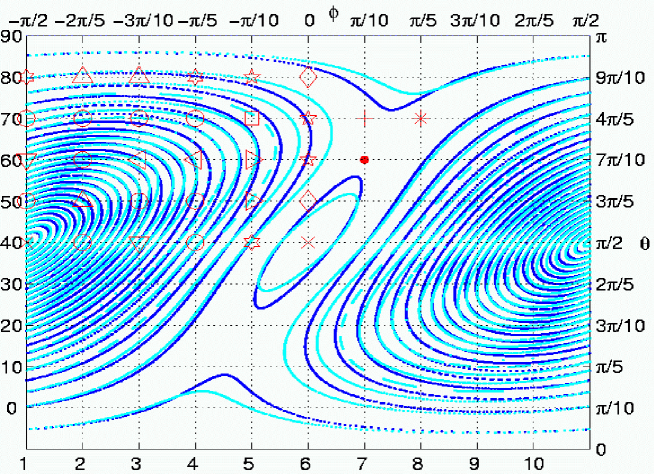
Figure 1: (Color online) Twenty-five classical orbits on the phase space of the classical kicked top, $k_{T}=1.1$ (dark), and $k_{T}=1.3$ (light). The same initial points are used to map the orbits so as to demonstrate the effect of the $\delta_{T}$ perturbation. The change of kick strength primarily affects the frequency of the orbits around the stable point at $(\phi=-\pi/2,\theta=\pi/2)$ ($\times$). Thus, under a $\delta_{T}$ perturbation, we expect coherent states placed there to exhibit a Gaussian fidelity decay The change of kick strength does affect the shape of the central tori around the $(\phi=0,\theta=\pi/2)$ ($\times$) fixed point. Thus, under the $\delta_{T}$ perturbation we expect coherent states centered in that region to exhibit a power-law fidelity decay. The same holds for the rotational tori at the edges of the phase space. The different markers delineate the fidelity decay behavior of coherent states centered at those points. The states marked by circles, up, down, left, and right pointing triangles, five-pointed stars, and six-pointed stars mark states that exhibit Gaussian decay behavior at different rates. While we offer no clear, a priori, determination of the decay rate, states centered on the same orbit tend to decay at similar rates. Though different orbits may also give rise to similar decay rates, the general trend is towards a slower Gaussian as the states move further from the $(\phi=-\pi/2,\theta=\pi/2)$ fixed point. Power-law fidelity decay rates depend on distance from areas with large tori distortions, the region surrounding the central fixed point and the dip in the rotational torus at the top and bottom of the figure. The closer a state is to these regions, the slower the power-law rate. Gaussian and power-law fidelity decays are shown in Fig. 2 where the shapes correspond to the markers used in this figure.

The quantum kicked top (QKT) H2 is defined by the Floquet operator

$$U_{QKT}=e^{-i\pi J_{y}/2}e^{-ik_{T}J_{z}^{2}/2J}.$$ (3)

where $J$ is the angular momentum of the top and ${\bf\vec{J}}$ are the irreducible angular momentum operators. The Hilbert space dimension of the top is $N=2J+1$. The representation is such that $J_{z}$ is diagonal. As initial states we use minimum uncertainty angular momentum coherent states centered around $(\phi_{i},\theta_{i})$ Peres2 and employ a QKT of $J=500$ unless otherwise noted.

For convenience we number the states assuming a 10 by 10 grid evenly spaced in the $\theta$ and $\phi$ directions as seen in Fig.  1. The lines of the grid are numbered such that the number of a state, centered at an intersection of the grid, is determined by adding the numerical values of the horizontal (numbers on left) and vertical (numbers on the bottom) lines. State 1 is thus located at ($\phi=-\pi/2$, $\theta=\pi/10$) and state 100 at ($\phi=2\pi/5$, $\theta=\pi$). In this way, the fixed point at $(\phi=-\pi/2,\theta=\pi/2)$ is number 41 while the fixed point at $(\phi=0,\theta=\pi/2)$ is number 46.

Fig. 2 shows that state 52, centered in the region of phase space surrounding the fixed point $(\phi=-\pi/2,\theta=\pi/2)$, exhibits the expected Gaussian behavior (triangles), and that state 66, near the fixed point $(\phi=0,\theta=\pi/2)$ (solid line), exhibits the expected power-law decay. These states parallel the expected classical fidelity decay behavior.

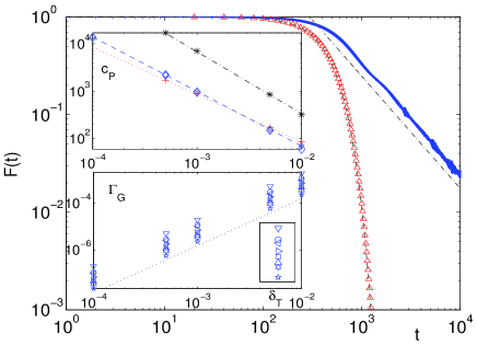
Figure 2: (Color online) Fidelity decay for quantum kicked top (QKT) with $k_{T}=1.1,\delta_{T}=.001$, and $J=500$, of two different coherent states. One (triangles) placed in the region of stable KAM tori surrounding the fixed point $(\phi=-\pi/2,\theta=\pi/2)$ (state 52, up triangle in Fig. 1, every 20 steps shown) where the perturbation effects a change in phase space orbit frequency, and the other (solid line) placed in the region surrounding the $(\phi=0,\theta=\pi/2)$ stable point (state 56, diamond in Fig. 1) where the perturbation causes a distortion of the phase space orbit. As expected, the former displays a Gaussian fidelity decay (dashed line), $e^{-\Gamma_{G}t^{2}}$, with $\Gamma_{G}=4.5\times 10^{-6}$, while the latter exhibits a power law decay $c_{P}t^{-\alpha_{P}}$ (dash-dotted line) with $\alpha_{P}=1.15$ and $c_{P}=950$. The insets show the change of fidelity decay rate as a function of perturbation strength, $\delta_{T}$. The top inset plots $\delta_{T}$ versus $c_{P}$ for states that decay as $\propto t^{-1}$ (+), $t^{-1.15}$ (diamond), and $t^{-1.3}$ (*) (as explained later, different coherent states decay with different power-laws). The points on the loglog plot are well fit by $c_{P}=.85\delta_{T}^{-1}$ (dotted line), $.35\delta_{T}^{-1.15}$ (dashed line) and $.85\delta_{T}^{-1.3}$ (dash-dotted line). From these and numerical results of other states we assume the following form for power law decay $F_{P}(t)=c_{P}(\delta_{T}t)^{-\alpha_{P}}$. The lower inset shows the change of the Gaussian rate, $\Gamma_{G}$, as a function of $\delta_{T}$ (marked by shapes corresponding to those in Fig. 1). As addressed below, coherent states centered in different areas of phase space exhibit different Gaussian decay rates, with the rate slowing as the states move further from the stable point. The dependence of the rate on perturbation strength, however, is always $\Gamma_{G}\propto\delta_{T}^{2}$ (dotted line).

The existence of states with power-law decay supports the contentions of Ref. P3 in explaining contradictory results in regular system fidelity decay behavior. These states bias the average to look like a power law which is slower than the exponential fidelity decay of chaotic systems. Many states, however, exhibit Gaussian fidelity decay which may, under certain circumstances, be faster than the decay of the corresponding chaotic fidelity.

The parallel between the fidelity of quantum states and their classical counterparts is not, however, the case in general. Some states initially centered in areas of apparent phase space orbit distortion exhibit the Gaussian fidelity decay expected from perturbations of an orbit’s frequency. We show this in the quantum version of the system explored classically by BCV Ben2 , the kicked rotor. The classical dynamics of the kicked rotor is given by

$$p_{t+1} = p_{t}+(k_{R}/2\pi)\sin(2\pi q_{t})$$

$$q_{t+1} = q_{t}+p_{t+1}$$ (4)

where $k_{R}$ is the rotor kick strength and $-1/2<q,p<1/2$. For $k_{R}=.3$ the phase space of the kicked rotor has a stable fixed point at $(q=-.5,p=0)$ ($\times$) and an unstable fixed point at $(q=0,p=0)$ (+). The phase space is divided into two distinct regions, orbits around the stable fixed point, and rotational motion, as shown in Fig. 3. The orbit at the border between these regions is the separatrix. As with the QKT we plot phase space orbits of different $k_{R}$ to demonstrate the effect of a change of kick strength perturbation on different parts of the classical phase space. The shapes of certain KAM tori, such as the ones just outside the separatrix, exhibit large deformations while others, such as the inner circles within the separatrix, do not. As shown in Ben2 , states in the former region exhibit Gaussian classical fidelity decay while those in the latter region exhibit power-law decay.

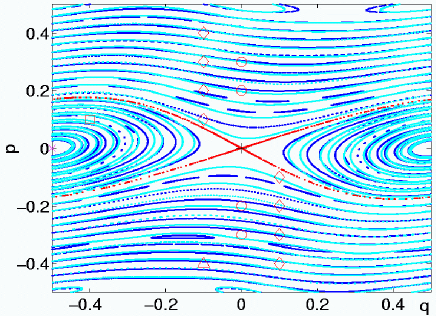
Figure 3: (Color online) Thirty orbits on the phase space of the classical kicked rotors, $k_{R}=.3$ (dark), and $k_{R}=.35$ (light). The same initial points are used to plot the orbits of both maps in order to highlight the effect of a $\delta_{R}$ perturbation. Well within the separatrix, the effect of the $\delta_{R}$ perturbation is generally to change the frequency of the KAM tori. Outside the separatrix, however, the $\delta_{R}$ perturbation essentially changes the shape of the tori. Also shown are the stable, $(q=-.5,p=0)$ ($\times$), and unstable, $(q=0,p=0)$ (+), fixed points and states used in the text to demonstrate Gaussian (square) and non-Gaussian (circle, diamond) fidelity decay. Classically, states outside the separatrix are expected to exhibit power-law fidelity decay. In the quantum realm, however, we find that many such states exhibit Gaussian decay, an example of which is marked by the triangle.

To study quantum fidelity decay of the kicked rotor, we use the unitary operator describing the quantum kicked rotor (QKR) L1

$$U_{QKR}=e^{-ip^{2}\pi N}e^{-ik_{R}\cos(2\pi q)N/\pi},$$ (5)

where $N$ is the Hilbert space dimension. For our simulations we use QKRs of $N=500,1000$, $k_{R}=.3$, corresponding to a classical kicked rotor with non-chaotic dynamics, and perturbation strengths $\delta_{R}=.002,.0014$. As initial states we use the minimum uncertainty coherent states described in Sar centered around $(q_{i},p_{i})$.

Fig. 4 shows the fidelity decay of quantum coherent states centered in different regions of phase space. One (squares) in a phase space region where the effect of $\delta_{R}$ is primarily to change the frequency of the KAM tori,$(q=-.4,p=.1)$ (square in Fig. 3), and another (solid line) in a phase space region where $\delta_{R}$ primarily distorts the shape of the KAM tori $(q=-.1,p=.1)$, (diamond in Fig. 3). The former exhibits a Gaussian fidelity decay while the latter exhibits a decay which is non-Gaussian and resembles (but is not quite) a power-law. An exact power-law does not emerge for any of the states simulated for the QKR even for perturbation strengths as low as $\delta_{R}=.0005$. Fig. 4 also shows a state, $(q=-.1,p=-.4)$, centered on a rotational orbit outside the separatrix which, despite the classical prediction of a power-law fidelity decay, exhibits Gaussian decay (triangle in Fig. 3).

As mentioned above, BCV Ben2 predict a lack of correspondence between classical and quantum fidelity decay noting that the quantization of KAM tori tends to suppress transitions between them. This would enforce a change of frequency as the primary effect of the perturbation. The lack of an actual power-law decay at any point in the QKR orbits implies such a suppression throughout the region of rotational motion. Lack of correspondence to classical dynamics for rotational QKR orbits has also been noted with respect to fidelity recurrences L1 . Fidelity recurrences, as seen in Fig. 4, are predicted classically in all regions of phase space. Yet, in the quantum realm, they do not occur in the QKR rotational tori. Ref. L1 notes that these regions have a high density of states and the enhanced quantum interference may cause the lack of classical correspondence. A similar argument can be proposed here, as enhanced quantum interference may be especially sensitive to perturbations and cause the fast Gaussian fidelity decay.

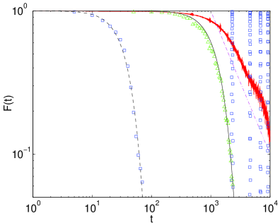
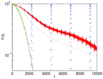
Figure 4: (Color online) Log-log and log-linear plots of three coherent state fidelity decay behaviors under evolution of the quantum kicked rotor with $k_{R}=.3,\delta_{R}=.002$, and $N=500$. One of the states is centered inside the separatrix at ($q=-.4,p=.1$) (squares every 50 time steps), where there is no apparent distortion of KAM tori. The location of this state on the classical phase space is marked by a square in Fig. 3. Another state is centered outside the separatrix ($q=-.1,p=.1$) (solid line, diamond in Fig. 3) where there is noticeable KAM tori distortion due to the perturbation. The former displays a Gaussian fidelity decay (dashed line), $e^{-.0006t^{2}}$ and exhibits fidelity recurrences every 2300 time steps L1 . The latter exhibits a decay which is non-Gaussian. A power-law $\propto t^{-1}$ (dash-dotted line) is plotted for comparison. The third state (triangle) is centered outside the separatrix (triangle in Fig. 3) but nonetheless exhibits a Gaussian decay $F(t)=e^{-5\times 10^{-7}t^{2}}$. This state does not exhibit fidelity decay recurrences.

In attempt to further understand what differentiates states that exhibit Gaussian fidelity decay from those that exhibit power-law decay we look at the spectra of the initial coherent states with respect to the QKT eigenbasis as a function of the extent of the eigenstates in $J_{z}$. Following Peres Peres2 the extent of a state with respect to the operator $J_{z}$ is defined as

$$\Delta|J_{z}|=\sqrt{\langle\psi|J_{z}^{2}|\psi\rangle-|\langle\psi|J_{z}|\psi\rangle|^{2}}.$$ (6)

The extent is basically the first term in the power series expansion of the fidelity Peres1 and thus we expect it to provide insight into the expected fidelity decay behavior. We calculate the extent of all the eigenstates of the QKT and see how much each of these states contributes to a given coherent state. The contribution is quantified by an amplitude $A_{j}=|\langle\psi_{i}|\phi_{j}\rangle|^{2}$ where $\psi_{i}$ is the initial coherent state and $\phi_{j}$ is the $j$th QKT eigenstate.

On the extremes, the coherent state centered at the stable fixed point $(\phi=-\pi/2,\theta=\pi/2)$ is primarily ($A=.95$) composed of one eigenstate with $\Delta|J_{z}|=17.3$. The primary contributors to the coherent state centered at the stable fixed point at $(\phi=0,\theta=\pi/2)$ are 4 eigenstates each with amplitudes of .21 and $\Delta|J_{z}|=353.7$. In both cases the fidelity barely decays as the state lives in a constricted Hilbert space Peres2 ; P1 ; YSW1 .

Most coherent states, however, have significant contributions from many different eigenstates. In Fig. 5 the contribution to coherent states 52-56 is plotted versus the extent of the eigenstates and in the inset the same is plotted for states 64-67. The general pattern emerging from the figure (and from states not shown) is clear. Coherent states exhibiting Gaussian fidelity decay have a Gaussian spectrum of contributions from eigenstates with low to middle range extents in $J_{z}$. As the coherent states move away from the low-extent $(\phi=-\pi/2,\theta=\pi/2)$ fixed point (with distance determined by the number of passing trajectories) more and more states contribute and with lower amplitudes, higher extent, and a more localized extent range. The Gaussian shape remains until the coherent states enter the region of power-law fidelity decay. States with power-law fidelity decay have a very narrow spectra at high extent. The difference between the types of states is clearly seen in Fig. 5 and the transition between the types of states can be seen in Fig. 7.

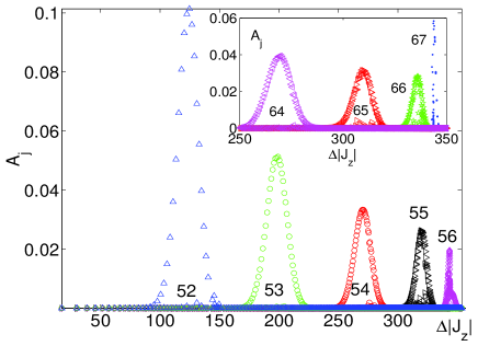
Figure 5: (Color online) Contribution of QKT eigenstates for coherent states 52-56 (left to right) versus extent of those eigenstates in $J_{z}$ with shapes as in Fig.  1. As the states move further from the low extent $(\phi=-\pi/2,\theta=\pi/2)$ fixed point more eigenstates have significant contributions and the height of the Gaussian contribution curve decreases. Consequently, the Gaussian fidelity decay rate decreases. State 56, made of only high-extent states, does not have a Gaussian extent spectrum and exhibits power-law fidelity decay. The inset shows coherent states 64-67 (left to right) which follow a similar pattern.

We suggest that the relationship between fidelity decay and the extent spectrum may be understood as follows. States exhibiting power-law decay have a large extent in the direction of the perturbation, $J_{z}$. When the coherent state is perturbed these states cannot spread out much more in the perturbation direction. Rather, they interfere with each other and the decay is slow. Coherent states exhibiting Gaussian decay, however, are spread out in extent space. The perturbation affects each of these states differently spreading them out in $J_{z}$ and causing a ballistic decay. As the coherent states move away from the low extent fixed point the average extent of these states grows and the Gaussian fidelity decay gets slower until the transition to power-law decay. This description holds for states in the Gaussian and power-law fidelity decay regions for the QKT phase space. States at the border between these regions and states very close to the fixed points have different extent spectra and, thus, exhibit fidelity decay behavior that is neither Gaussian nor power-law. These regions will be discussed below.

A full exploration of the extent and its relation to fidelity decay is beyond the scope of this paper. However, looking at the spectrum of a coherent state as a function of the extent of the contributing basis states with respect to the perturbation operator, $V$ (or some function thereof), can help identify the regions of different decay behaviors.

We now embark on a more extensive exploration of coherent state fidelity decay behavior in the regular regime of the QKT. To this aim, we have calculated the fidelity decay for coherent states spaced throughout the classical phase space for a number of perturbation strengths and Hilbert space dimensions. A large variety of behaviors exist, though we concentrate only on the initial decay before any fidelity recurrences. In attempt to organize the data in a straightforward fashion we explore fidelity decay as it relates to the following variables: perturbation strength, Hilbert space dimension, and position of the initial state with respect to the underlying classical phase space. We also study hitherto unobserved exponential decay which may occur after an initial Gaussian decay and explore how this decay regime behaves with respect to the above variables. We note that an extensive semi-classical treatment of regular fidelity decay has been done in Ref. P1 . Our purpose here is to outline an approach based on knowledge of the system’s classical phase space.

We first address the dependence of the fidelity decay rate as a function of perturbation strength. For coherent states exhibiting a Gaussian fidelity decay, $F_{G}(t)=e^{-\Gamma_{G}t^{2}}$, numerical simulations verify $\Gamma_{G}\propto\delta_{T}^{2}$, as derived in P1 . This dependence is demonstrated in the lower inset of Fig. 2 for $\delta_{T}=.0001,.0005,.001,.005,.01$ and $J=500$. For coherent states exhibiting a power law decay, $F_{P}(t)=c_{P}t^{-\alpha_{P}}$, numerical results for the above perturbation strengths suggest that $c_{P}$ is $\propto\delta_{T}^{-\alpha_{P}}$, from which we conclude $F_{P}(t)=c(\delta_{T}t)^{-\alpha_{P}}$. The upper inset in Fig. 2 demonstrates this behavior with states whose power-law decay rate is $\alpha_{P}=1,1.15,$ and $1.3$.

To address the fidelity decay behavior as a function of Hilbert space dimension we choose one perturbation strength, $\delta_{T}=.005$, for $J=100,200,300,400,500$. The fidelity decay is calculated for coherent states of appropriate dimension centered at specified points in phase space. For states centered in regions of Gaussian fidelity decay we find a linear relation between $J$ and $\Gamma_{G}$, as shown in the inset of Fig. 6, the slope of which depends on the coherent state’s location in phase space.

We can thus write the following equation for the Gaussian fidelity decay behavior:

$$F_{G}(t)=e^{-\Gamma_{G}t^{2}},\;\;\;\;\;\;\;\;\Gamma_{G}=\gamma_{G}J\delta^{2}$$ (7)

where $\gamma_{G}$ depends only on the initial coherent state’s location in phase space and is the only term not a priori calculable from our analysis. This result is in consonance with the semi-classical approach outlined in P1 .

For coherent states in regions of power-law fidelity decay, we find no change in decay rate with $J$ as long as the fidelity decay remains a power-law. Thus we write the following equation for the power-law decay behavior

$$F_{P}(t)=c(\delta_{T}t)^{-\alpha_{P}}$$ (8)

where $c$ and $\alpha_{P}$ depend on the coherent state’s location. However, as $J$ is decreased the fidelity decay behavior does change; it shifts from power-law to Gaussian, as shown in Fig. 6 (for state 56, marked diamond in Fig. 1). This shift is due to the increasing size of the initial coherent state making it more likely that the states will overlap with KAM tori on whom the perturbation effects a change of frequency. Coherent states centered more deeply in the power law decay region (such as state 77 marked plus in Fig. 1) have a slower transition to Gaussian decay when decreasing $J$.

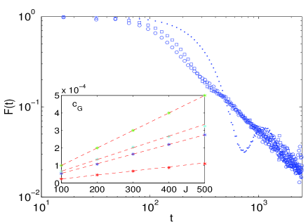
Figure 6: (Color online) Coherent state 56 (diamond in Fig. 1) power-law fidelity decay (every 16th time step plotted) for the QKT with $k_{T}=1.1$, $\delta_{T}=.005$, and $J=500$ (circles), 300 (squares), and 100 (dots). Lowering $J$ causes the fidelity decay behavior to transition from power law to Gaussian. The inset shows the rate of Gaussian fidelity decay, $\Gamma_{G}$, as a function of $J$ for some coherent states. We find a linear relationship $\Gamma_{G}=c_{G}J$ with $c_{G}=2.3\times 10^{-7}$, $5.5\times 10^{-7}$, $6.7\times 10^{-7}$ and $1\times 10^{-6}$ (bottom to top) shown.

As we have seen, the fidelity decay behavior in general, and the rate of $F_{G}(t)$ and $F_{P}(t)$ specifically, are dependent on the exact location of the initial coherent state with respect to the underlying classical phase space. This dependence is emphasized in Fig. 1 by using different shapes to mark the center of coherent states exhibiting Gaussian (circle, square, up, down, left, and right triangles, five-pointed star, and six-pointed star) and power-law (diamond, +, dot, *) fidelity decay. States with practically equivalent decay rates are represented by the same shape, with the rates themselves shown in Fig. 2. Based on our simulations we cannot formulate clear cut rules for the decay rate of a given coherent state. However, we make two observations. First, states along the same phase space orbit tend to have similar decay rates. Second, $\Gamma_{G}$, the rate of Gaussian decay, decreases as the states get further from the $(\phi=-\pi/2,\theta=\pi/2)$ fixed point (with distance measured by the number of trajectories between the fixed point and the center of the coherent state). We have already seen consequences of this latter observation in the extent spectra. Similarly, for states exhibiting power-law decay behavior, the power increases as the states get further from regions of large KAM torus distortion.

We now explore the fidelity decay of states at the border between the Gaussian and power-law phase-space regions and of states close to the fixed points. These regions exhibit a variety of decay behaviors which are reflected in the extent spectrum. Looking at the transition from Gaussian to power-law decay away from the fixed points we note that the transition is a rather smooth one in both the decay behavior itself and the extent of the contributing eigenstates. Fig. 7 displays these behaviors for coherent states $\theta=4\pi/5$ and $\phi$ ranging from $0$ to $\pi/10$ (between states 76 and 77 of Fig. 1). For the fidelity, the decay slows as the state leaves the region where the dominant perturbation effect is on the frequency of the orbits and enters the region where the dominant perturbation effect is on the shape of the orbits. In the extent spectra the transition is manifest by the Gaussian shape narrowing on the side of large extent eventually becoming almost flat except for a tail reaching towards the higher extent eigenstates. Similar behavior is found for other states in the border region between Gaussian and power-law fidelity decay.

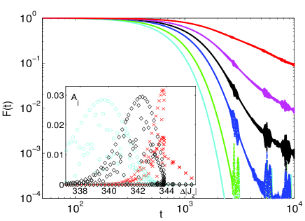
Figure 7: (Color online) Fidelity decay of coherent states with $\theta=4\pi/5$ and $\phi$ ranging from $0$ (state 76) and $\pi/10$ (state 77) for the QKT with $k_{T}=1.1$, $\delta_{T}=.001$. The states shown are for $\phi=\pi/100,3\pi/100,5\pi/100,6\pi/100,7\pi/100$, and $9\pi/100$ (bottom to top). The decay can be seen to transition smoothly from Gaussian to power-law. The inset shows the extent spectrum of the states at $\phi=3\pi/100$ (circles), $6\pi/100$ (diamonds), and $9\pi/100$ ($\times$). As the power-law fidelity decay region is approached, the Gaussian spectrum gets filled in and narrows on the side of higher extent becoming almost flat except for a tail of high-extent states.

The region surrounding the $(\phi=0,\theta=\pi/2)$ fixed point contains states exhibiting fidelity decay behaviors not described by a Gaussian or power-law and extent spectra different from those seen above. Starting with the coherent state centered at the fixed point, the fidelity oscillates close to one as the coherent state is comprised almost entirely of the highest extent QKT eigenstates. As the coherent states move away from the fixed point the highest extent eigenstates still gives the largest contributions while the next highest extent eigenstates give increased contributions. The fidelity decay in these regions starts off as a power-law but exhibits a second stage of Gaussian decay similar to edge of quantum chaos decays YSW2 . Moving further, eigenstates with lower and lower extent become dominant. However, the extent spectrum is not Gaussian, as would be expected for states exhibiting Gaussian fidelity decay, but is extended on the side of lower extent eigenstates. At this increased distance from the fixed point, the first-stage fidelity decay transitions from power-law to Gaussian, and the second-stage decay transitions from Gaussian to power-law decay. Finally, the initial Gaussian fidelity decay flattens into one stage of power-law decay while the extent spectrum continues flattening in the direction of higher extent states while forming a complicated flattened bulge at lower extent states. All of these behaviors are exhibited in Fig. 8. Similar behavior is found in regions of coherent states 3-5 and 87-89.

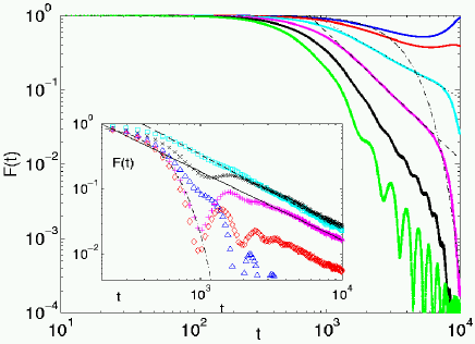
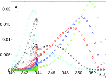
Figure 8: (Color online) The top panel shows the fidelity decay of coherent states with $\theta$ ranging from $\pi/2$ to $6\pi/10$ and $\phi=0$ for the QKT with $k_{T}=1.1$, $\delta_{T}=.001$. The states shown are for $\theta=\pi/2+0,\pi/100,2\pi/100,3\pi/100,4\pi/100$, and $5\pi/100$, (top to bottom). Close to the fixed point the fidelity oscillates close to one. As the states move further away from the fixed point, the fidelity decays in two stages, starting as a power-law and becoming a Gaussian. For comparison we fit the initial decay of the $\theta=\pi/2+2\pi/100$ state with a power-law $\propto t^{-1}$ (dotted line), the $\theta=\pi/2+3\pi/100$ state initial decay with a power-law $\propto t^{-1.7}$ (dashed line), and the second stage decay with a Gaussian $e^{-\Gamma_{ss}t^{2}}$ with $\Gamma_{ss}=8\times 10^{-8}$ (chained line). Moving further away, the initial power-law becomes more Gaussian while the second stage starts flattening to power-law. The inset shows every 60 steps of the fidelity decay for the states $\phi=0$, $\theta=\pi/2+6\pi/10$ (triangles), $7\pi/100$ (diamonds), $8\pi/100$ (+), $9\pi/100$ ($\times$), and $\pi/10$ (state 56, squares). Here, the initial decay starts off as Gaussian and rebounds into a power-law decay. For comparison we plot the Gaussian $e^{-\Gamma_{G}t^{2}}$ with $\Gamma_{G}=3.9\times 10^{-6}$ (chained line) and the power-law $\propto t^{-1.05}$ (solid line) . As the states continue to move away from the fixed point, however, the Gaussian flattens until there is a single-behavior power-law decay, $\propto t^{-1.15}$ (dashed line). The lower panel shows the extent spectrum of the states with $\theta=\pi/2+5\pi/10$ (o), $6\pi/10$ (triangles), $7\pi/10$ (diamonds), $9\pi/10$ ($\times$), and state 56 (squares). As the coherent states are moved further away from the fixed point the spectra flatten at higher extent eigenstates and a bulge grows at lower extent eigenstates.

Coherent states in the region surrounding the fixed point at $(\phi=-\pi/2,\theta=\pi/2)$ exhibit behavior that is slightly different from the states in the region surrounding the $(\phi=0,\theta=\pi/2)$ fixed state. At the fixed point the fidelity simply oscillates close to 1. As the coherent states move away from the fixed point the oscillations become larger in amplitude, the recurrence time increases, the initial decay becomes more Gaussian, and the maximum fidelity reached on the recurrence is lower. This continues until full Gaussian decay behavior emerges. The extent spectra reflect this behavior, going from a dominant low extent state to an eventual Gaussian shape.

We also note the presence of states with unexpected fidelity decay behavior in the QKR. Fig. 9 shows examples of $N=1000$ coherent states under QKR $k_{R}=.3$, $\delta_{R}=.0014$ evolution that exhibit initial exponential fidelity decay (top plot), though the QKR is regular, and fidelity ‘freeze’ as discussed in Ref. P3 , though the perturbation is non-ergodic.

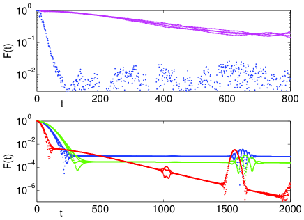
Figure 9: (Color online) The upper plot shows two coherent states evolved under the $N=1000$, $k_{R}=.3$ QKR with $\delta_{R}=.0014$ that exhibit initial exponential decay despite the fact that the QKR is in the regular regime. The lower plot shows three coherent states under the same QKR evolution which exhibit initial Gaussian decay that transitions to exponential decay. For two of the states the fidelity freezes after the initial Gaussian decay. The fidelity of all three states exhibit echo resonances similar to those discussed in Ref. P3 for ergodic perturbations.

Beyond the initial Gaussian fidelity decay of some coherent states, there may exist a second, slower, stage of exponential fidelity decay behavior, $F(t)=c_{E}e^{-\beta_{E}}$, before saturation. This stage is prevalent for strong perturbations but disappears for smaller perturbations (or smaller Hilbert space dimension with the same perturbation strength). The specifics of this exponential decay depend strongly on the phase space location of the initial coherent state. The slower exponential decay of this second stage gives rise to an exciting phenomenon: a stronger perturbation leading to a higher fidelity than a weaker perturbation of the same type.

The golden rule exponential fidelity decay term mentioned above for chaotic systems exists also in regular systems J3 . We do not identify this term with the exponential observed here since, as we show, the exponential here is strongly dependent on the initial state.

As with the initial fidelity decay behavior we attempt a systematic numerical analysis of the second stage exponential decay. We first study the exponential as a function of perturbation and then explore the effect of the location of the initial coherent state.

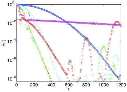
Figure 10: (Color online) Coherent state 54 (circle in Fig. 1) fidelity decay (every 5th time step plotted) for the QKT with $k_{T}=1.1$, and $J=500$, for perturbation strengths $\delta_{T}=.01$ (squares), $.0075$ (diamonds), $.005$ (triangles), $.0025$ (+), and $.001$ (o). The fidelity decay of the stronger perturbations show a stage of exponential decay after the initial Gaussian. This stage is fitted by $F(t)=12e^{-.035t}$ (dash-dotted line) for $\delta_{T}=.01$, $F(t)=.025e^{-.00115t}$ (solid line) for $\delta_{T}=.0075$, and $F(t)=7e^{-.052t}$ (dashed line) for $\delta_{T}=.005$. For the strongest perturbations, $\delta_{T}=.01,.0075$, there is also a period of transfer between the two fidelity decay regimes, while for $\delta=.005$ this transition period is non-existent. For weaker perturbations the exponential stage of fidelity decay disappears altogether. The faster Gaussian decay of the weaker perturbations and the wide range of exponential decay rates, leads to the counter-intuitive result that a stronger perturbation leads to a higher fidelity as seen in the region $200<t<600$ for the $\delta_{T}=.01$ decay and across the whole plotted region for the $\delta_{T}=.0075$ decay. There is no clear correlation between perturbation strength and exponential decay rate.

Fig. 10 demonstrates that weaker perturbations (+,o) exhibit no exponential fidelity decay stage. Rather, the Gaussian decay continues until fidelity saturation. As the perturbation strengthens the second-stage exponential emerges. In addition, there exists a transition period between the two decay behaviors. Thus, weaker perturbations lead to longer times of Gaussian fidelity decay during which the fidelity of stronger perturbations may have already transferred to the slower exponential. In this way, there may be a significant amount of time in which the fidelity of the stronger perturbation (diamonds, triangles) is actually higher than that of the weaker perturbation (squares, +). This phenomenon is shown in Fig. 10 for the $k_{T}=1.1$, $J=500$, QKT. An exponential region of decay is manifest for perturbation strengths $\delta_{T}=.01,.0075,$ and $.005$, but not for weaker perturbations $\delta_{T}=.0025$ and $.001$. Thus, for times $t>300$ the fidelity of at least one of the stronger perturbations is higher than the fidelity of a weaker perturbation.

The rate of the exponential also depends on the perturbation strength, $\delta_{T}$. However, our numerical simulations do not show any simple relationship between the exponential rate and the perturbation strength. Rather, the rate changes drastically ranging from practically zero, decay freeze, to a fast exponential. This also allows a stronger perturbation to have a higher fidelity than a weaker one. This is exemplified in Fig. 10 by the $\delta=.0075$ perturbation whose fidelity decays very slowly and, thus, after a time, is higher than the fidelity of all of the weaker perturbations.

The possibility of a stronger perturbation leading to a higher fidelity may have important consequences for quantum simulations in which a quantum system is trying to simulate a given dynamics: a strong error in the dynamics may be easier to correct via quantum error correction than a weak one. This could allow for an interesting error-correction scenario. A weak error strongly affecting a system should be purposely strengthened so as to more accurately perform the desired simulation. This would be especially significant in a case where the effect of the error is too strong for conventional quantum error techniques but can be brought below the error-correction threshold if the error is strengthened.

The existence of the exponential fidelity decay region may be related to the quantum freeze of fidelity discussed in P3 for ergodic perturbations. In fact, the lower plot of Fig. 9 displays the fidelity decay of coherent states evolved by the QKR which actually freeze, though the applied perturbation is non-ergodic.

The region of exponential fidelity decay varies dramatically with the location of the coherent state on the underlying classical phase space. This is displayed in Fig. 11 where a wide range of exponential decay rates are found for different coherent states though they undergo equivalent evolution. In addition, the time of the transition period from Gaussian to exponential varies from state to state.

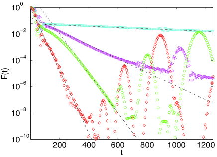
Figure 11: (Color online) Fidelity decay for different coherent states (every 5th time step plotted) for the quantum kicked top with $k_{T}=1.1$, $J=500$, and $\delta_{T}=.01$. After the initial Gaussian the fidelity decay transitions to an exponential, the rate of which depends strongly on the location of the coherent state with respect to the underlying classical phase space. The states shown are 53 (diamonds), 54 (o), 55 (triangles), and 74 (squares). All of these states have initial Gaussian fidelity decay, as seen in Fig. 2, which transitions into an exponential decay. The current figure exhibits the wide range of exponential decay rates and transition times that can occur. Starting with the lowest plot we find exponential decays of $F(t)=e^{-.055t}$ (diamonds), $10e^{-.0345t}$ (circles), $.175e^{-.012t}$ (triangles), and $.06e^{-.00011t}$ (squares). These exponentials are displayed by dashed lines in the figure.

In conclusion, we have provided a numerical study of fidelity decay behavior for coherent states in a quantum system whose classical analog is quasi-integrable. We find that the initial fidelity decay behavior and rate will depend on the perturbation strength, Hilbert space dimension, and initial coherent state location. The quantum fidelity decay behavior generally corresponds to the classical fidelity decay explored in Ben2 and the prediction therein: quantum states tend more towards Gaussian decay due to the quantization of the phase space orbits. In addition, we show that the spectrum of the initial coherent state with respect to the system eigenstate extent contains information regarding the fidelity decay of that state. Finally, we find that after initial Gaussian decay behavior, there may be a second stage of exponential decay for strong perturbations. The rate and inception of the exponential decay depend on the perturbation strength and location of the coherent state. The existence of this second-stage decay behavior leads to the counter-intuitive result that stronger perturbations may lead to higher fidelity, a phenomenon which may be important for quantum computation.

The authors acknowledge support from the DARPA QuIST (MIPR 02 N699-00) program. Y.S.W. acknowledges the support of the National Research Council Research Associateship Program through the Naval Research Laboratory. Computations were performed at the ASC DoD Major Shared Resource Center.

References

- (1) F. Haake, Quantum Signatures of Chaos (Springer, New York, 1991).
- (2) A. Peres, Phys. Rev. A 30, 1610, (1984).
- (3) A. Peres, in Quantum Chaos, ed. H.A. Cerdeira, R. Ramaswamy, M.C. Gutzwiller, G. Casati, (World Scientific, Singapore, 1991), page 73; A. Peres, Quantum Theory: Concepts and Methods, (Kluwer Academic Publishers, Dordrecht, 1995).
- (4) W.K. Rhim, A. Pines, J.S. Waugh, Phys. Rev. Lett. 25, 218, (1970); Phys. Rev. B 3, 684, (1971); S. Zhang, B.H. Meier, R.R. Ernst, Phys. Rev. Lett. 69, 2149, (1992).
- (5) P.R. Levstein, G. Usaj, H.M. Pastawski, J. Chem. Phys. 108, 2718, (1998).
- (6) G. Usaj, H.M. Pastawski, P.R. Levstein, Mol. Phys. 95, 1229, (1998).
- (7) R.A. Jalabert and H.M. Pastawski, Phys. Rev. Lett. 86, 2490, (2001).
- (8) Ph. Jacquod, P.G. Silvestrov, C.W.J. Beenakker, Phys. Rev. E 64, 055203(R), (2001).
- (9) F.M. Cucchietti, C.H. Lewenkopf, E.R. Mucciolo, H.M. Pastawski, R.O. Vallejos, Phys. Rev. E, 65, 046209, (2002).
- (10) J. Vanicek, E.J. Heller, Phys. Rev. E 68, 056208, (2003).
- (11) T. Prosen, M. Znidaric, J. Phys. A 35 1455, (2002).
- (12) Ph. Jacquod, I. Adagideli, C.W.J. Beenakker, Phys. Rev. Lett. 89, 154103, (2002).
- (13) J. Emerson, Y.S. Weinstein, S. Lloyd, D.G. Cory, Phys. Rev. Lett., 89, 284102, (2002).
- (14) D.A. Wisniacki, E.G. Vergini, H.M. Pastawski, F.M. Cucchietti, Phys. Rev. E 65, 055206(R), (2002).
- (15) N.R. Cerruti and S. Tomsovic, Phys. Rev. Lett. 88, 054103 (2002).
- (16) N.R. Cerruti, S. Tomsovic, J. Phys. A, 36, 3451, (2003).
- (17) W. Wang, B. Li, Phys. Rev. E, 66, 056208, (2002).
- (18) Y.S. Weinstein, J. Emerson, S. Lloyd, D.G. Cory, Quant. Inf. Proc., 6, 439, (2003).
- (19) D.A. Wisniacki, Phys. Rev. E 67, 016205, (2003).
- (20) W.G. Wang, G. Casati, B. Li, Phys. Rev. E, 69, 025201(R), (2004).
- (21) Y. S. Weinstein, S. Lloyd, C. Tsallis, Phys. Rev. Lett., 89, 214101 (2002); Y.S. Weinstein, C. Tsallis, S. Lloyd, in Decoherence and entropy in Complex Systems, ed. H.-T. Elze, Lecture Notes in Physics 633, (Springer, Berlin, 2004), page 385.
- (22) D.A. Wisniacki, D. Cohen, Phys. Rev. E, 66, 046209, (2002).
- (23) G. Benenti, G. Casati, Phys. Rev. E, 65, 066205, (2002).
- (24) M. Hiller, T. Kottos, D. Cohen, T. Geisel, Phys. Rev. Lett., 92, 010402, (2004).
- (25) F.M. Cucchietti, D.A.R. Dalvit, J.P. Paz, W.H. Zurek, Phys. Rev. Lett. 91, 210403, (2003).
- (26) D. Poulin, R. Blume-Kohout, R. Laflamme, H. Ollivier, Phys. Rev. Lett., 92, 177906, (2004).
- (27) Y.S. Weinstein, S. Lloyd, J. Emerson, D.G. Cory, Phys. Rev. Lett., 89, 157902, (2002).
- (28) B. Eckhardt, J. Phys. A, 36, 371, (2003).
- (29) G. Benenti, G. Casati, G. Veble, Phys. Rev. E, 67, 055202(R), (2003).
- (30) G. Veble, T. Prosen, Phys. Rev. Lett., 92, 034101, (2004).
- (31) T. Prosen, M. Znidaric, New J. Phys., 5, 109, (2003).
- (32) R. Sankaranarayanan, A. Lakshminarayan, Phys. Rev. E, 68, 036216, (2003).
- (33) P. Jacquod, I. Adagideli, C.W.J. Beenakker, Europhys. Lett., 61, 729, (2003).
- (34) T. Prosen, Phys. Rev. E, 65, 036208, (2002).
- (35) G. Benenti, G. Casati, G. Veble, Phys. Rev. E, 68, 036212, (2003).
- (36) F. Haake, M. Kus, R. Scharf, Z. Phys. B, 65, 381, 1987.
- (37) M. Saraceno, Ann. Phys., 199, 37, (1990).