Phase delay time and superluminal propagation in barrier tunneling

Abstract

In this work we study the behaviour of Wigner phase delay time for tunneling in the reflection mode. Our system consists of a circular loop connected to a single wire of semi-infinite length in the presence of Aharonov-Bohm flux. We calculate the analytical expression for the saturated delay time. This saturated delay time is independent of Aharonov- Bohm flux and the width of the opaque barrier thereby generalizing the Hartman effect. This effect implies superluminal group velocities as a consequence. We also briefly discuss the concept called “space collapse or space destroyer”.

I INTRODUCTION

Quantum tunneling is one of the most important phenomenon with wide range of applications in modern technology. In spite of its remarkable success in various applications, there still remains the fundamental question, namely, how much time does a particle take to traverse the barrier? ( so called tunneling time problem). This problem has been approached from many different viewpoints, but still there is a lack of consensus about the existence of simple expression for this time landauer ; hauge ; recami . This is due to the fact that there is no Hermitian operator associated with this time. The various time scales proposed in the literature are based on different operational definitions and physical interpretations. They may represent different complimentary aspect of tunneling process. Some of them include dwell time, Larmor time, complex times, Buttiker- Landauer times, sojourn times anantha , time scale based on Bohm’s view jayan1 , phase delay time, etc.

In our present work we concentrate mainly on the concept of Wigner phase delay time. This time is usually taken as the difference between the time at which the peak of the transmitted packet leaves the barrier and the time at which the peak of the incident Gaussian wave packet arrives at the barrier. Within the stationary phase approximation the phase time can be calculated from the energy derivative of the ‘phase shift’ in the transmitted or reflected amplitudes. This phase delay time is also related to various physical quantities such as partial density of states buttiker . In the case of a quantum tunneling it has been shown that in the opaque barrier limit the phase delay time does not depend on the barrier width. This phenomenon is called as the Hartman effect. This implies that for sufficiently large barriers the effective velocity of the particle can become arbitrarily large, even larger than the speed of light in the vacuum (superluminal). This may be further regarded as the evidence of the fact that quantum systems seem to behave as non-local. Experiments have clearly demonstrated steinberg ; nimtz ; expt that “tunneling photons” travel with superluminal group velocities. Their measured tunneling time is practically obtained by comparing the two peaks of the incident and transmitted wave packets. It is important to note that these observations do not violate ‘Einstein causality’, i.e., the signal velocity or the information transfer velocity is always bounded by the velocity of light. Theoretically Hartman effect has been generalized to different cases including double barriers, various geometric structures and in the presence of Aharonov-Bohm flux. Mystery surrounding this effect has also been addressed recently by Winful. He argues that the short time delay observed is due to energy storage and release and has nothing to do with propagation. Since the stored energy or the probability density in the evanescent field decreases exponentially with the distance in the barrier, after certain decay distance it does not matter how much more length the barrier has. For details we refer to winful .

In our present work we study the above mentioned effect in a simple quantum system consisting of a circular loop connected to a single wire of semi-infinite length as shown in Fig 1. In addition we impose Aharonov-Bohm flux through the loop. We also focus on the following situation. There is a potential barrier (or barriers) inside the loop, while the potential in the connecting lead is set to zero. The incident energy of the free propagating electron $E$ in the semi-infinite wire is less than the barrier potential height $V$. The impinging electron on the loop in the sub barrier region travels as an evanescent wave in the loop before being reflected. We analyze the phase time of the reflected wave. We show that this phase time in the opaque barrier regime becomes independent of the length of the circumference of the ring and the magnitude of the Aharonov-Bohm flux, thereby generalizing the Hartman effect beyond one dimension and in the presence of magnetic flux. We have also extended this effect by including an additional potential well in the circular ring. Interestingly the saturated delay time becomes independent of the length of the potential well (in the large length limit) in the off resonant case. The potential well can support many resonant states. This result is regarded as a “space collapse or space destroyer” recami2 . Even though in the potential well inside the loop electronic wave can travel as a free propagating mode (and not as a evanescent mode), surprisingly the saturated delay time is independent of the length of the well (as if it does not count).

In the sections to follow we first give the description of the theoretical treatment. For this we make use of the quantum waveguide approach well known for the electronic transport problems. The classical relativistic Helmholtz equation for the electromagnetic wave propagation is formally identical to non relativistic stationary Schrödinger equation. Hence conclusions obtained using quantum tunneling theory are equally valid in the case of electromagnetic phenomenon ( photon tunneling ). In the later sections we will discuss our results and conclusions.

Figure 1: Schematic diagram of a circular loop connected to semi infinite lead.

II THEORETICAL TREATMENT

We approach this scattering problem using the quantum wave guide theory  xia ; jayan3 . In the stationary case the incoming particles are represented by a plane wave $e^{ikx}$ of unit amplitude. The effective mass of the propagating particle is $m$ and the energy is $E=\hbar^{2}k^{2}/2m$ where $k$ is the wave vector corresponding to the free particle. The wave function in different regions (which are solutions of the Schrödinger equation) in the absence of magnetic flux are given below

$$\psi_{0}(x_{0}) = e^{ikx_{0}}+Re^{-ikx_{0}}\,\,\,\,\,\mbox{( in region I )}$$ (1)

$$\psi_{1}(x_{1}) = A_{1}\,e^{i\,q_{1}\,x_{1}}+B_{1}\,e^{-i\,q_{1}\,x_{1}}\,\,\,\,\,\mbox{( in region II )}$$ (2)

$$\psi_{2}(x_{2}) = A_{2}\,e^{i\,k\,x_{2}}+B_{2}\,e^{-i\,k\,x_{2}}\,\,\,\,\,\mbox{( in region III) }$$ (3)

$$\psi_{3}(x_{3}) = A_{3}\,e^{i\,q_{3}\,x_{3}}+B_{3}\,e^{-i\,q_{3}\,x_{3}}\,\,\,\,\,\mbox{( in region IV) }$$ (4)

with $k$ being the wavevector of electrons in the lead and in the intermediate free space between two barriers inside the ring. $q_{1}=\sqrt{2m(E-V_{1})/\hbar^{2}}$ and $q_{3}=\sqrt{2m(E-V_{3})/\hbar^{2}}$ are the wavevector respectively for propagating electrons in the barriers of strength $V_{1}$ and $V_{3}$ inside the ring. The origin of the co-ordinates of $x_{0}$ and $x_{1}$ is assumed to be at $J$ and that for $x_{2}$ and $x_{3}$ are at $P_{1}$ and $P_{2}$ respectively. At $P_{1}$, $x_{1}=lb_{1}$, at $P_{2}$, $x_{2}=w$ and at $J$, $x_{3}=lb_{3}$, where $lb_{1}$ and $lb_{3}$ are the length of the two barriers separated by a well region of length $w$ inside the ring. Total circumference of the ring is $L=lb_{1}+lb_{3}+w$.

We use Griffith’s boundary conditions griffith

$$\psi_{0}(0)=\psi_{1}(0)=\psi_{3}(lb_{3})\,$$ (5)

and

$$\frac{\partial\psi_{0}(x_{0})}{\partial x_{0}}\Big{|}_{J}+\frac{\partial\psi_{1}(x_{1})}{\partial x_{1}}\Big{|}_{J}+\frac{\partial\psi_{3}(x_{3})}{\partial x_{3}}\Big{|}_{J}=0\,,$$ (6)

at the junction $J$. All the derivatives are taken either outward or inward from the junction xia . Similar boundary conditions are held at $P_{1}$ and $P_{2}$ i.e.

$$\mbox{at \, \, $P_{1}$ \,:}\,\,\,\,\,\,\,\,\,\,\,\,\,\,\psi_{1}(lb_{1})=\psi_{2}(0)$$ (7)

$$\frac{\partial\psi_{1}(x_{1})}{\partial x_{1}}\Big{|}_{P_{1}}+\frac{\partial\psi_{2}(x_{2})}{\partial x_{2}}\Big{|}_{P_{1}}=0\,,$$ (8)

$$\mbox{at \, \, $P_{2}$ \,:}\,\,\,\,\,\,\,\,\,\,\,\,\,\,\,\psi_{1}(w)=\psi_{3}(0)$$ (9)

$$\frac{\partial\psi_{2}(x_{2})}{\partial x_{1}}\Big{|}_{P_{2}}+\frac{\partial\psi_{3}(x_{3})}{\partial x_{3}}\Big{|}_{P_{2}}=0\,.$$ (10)

We choose a gauge for the vector potential in which the magnetic field appears only in the boundary conditions rather than explicitly in the Hamiltonian xia ; gefen . Thus the electrons propagating clockwise and anticlockwise will pick up opposite phases. The electrons propagating in the clockwise direction from $J$ will pick up phases $i\,\alpha_{1}$ at $P_{1}$, $i\,(\alpha_{1}+\alpha_{2})$ at $P_{2}$ and $i\,(\alpha_{1}+\alpha_{2}+\alpha_{3})$ at $J$ after traversing once along the loop. The total phase around the loop is $\alpha_{1}\,+\,\alpha_{2}\,+\,\alpha_{3}\,=\,2\,\pi\,\phi/\phi_{0}$, where $\phi$ and $\phi_{0}$ are the magnetic flux and flux quantum, respectively. Hence from above mentioned boundary conditions we get for tunneling particle

$$1+R-A_{1}-B_{1}\exp(-i\,\alpha_{1})=0\,,$$ (11)

$$A_{3}\,\exp(-\kappa_{3}\,lb_{3})\,\exp(i\alpha_{3})+B_{3}\,\exp(\kappa_{3}\,lb_{3})-1-R=0\,,$$ (12)

$$ik\,(1-R)+\kappa_{1}\,(A_{1}-B_{1}\,\exp(-i\,\alpha_{1}))\hskip 56.9055pt$$

$$-\,\kappa_{3}\,A_{3}\,\exp(-\kappa_{3}\,lb_{3})\,\exp(i\,\alpha_{3})-\,\kappa_{3}\,B_{3}\,\exp(\kappa_{3}\,lb_{3})=0\,,$$ (13)

$$A_{1}\,\exp(-\kappa_{1}\,lb_{1})\,\exp[i\,\alpha_{1}]+B_{1}\,\exp(\kappa_{1}\,lb_{1})\hskip 56.9055pt$$

$$-\,A_{2}-B_{2}\,\exp(-i\,\alpha_{2})=0\,,$$ (14)

$$\kappa_{1}\,A_{1}\,\exp(-\kappa_{1}\,lb_{1})\,\exp(i\,\alpha_{1})-\kappa_{1}\,B_{1}\,\exp(\kappa_{1}\,lb_{1})\hskip 28.45274pt$$

$$+\,i\,k\,A_{2}-i\,k\,B_{2}\,\exp(-i\alpha_{2})=0\,,$$ (15)

$$A_{2}\,\exp(i\,k\,w)\,\exp(i\,\alpha_{2})\,+\,B_{2}\,\exp(-i\,k\,w)\hskip 56.9055pt$$

$$-\,A_{3}-B_{3}\,\exp(-i\alpha_{3})=0\,,$$ (16)

$$i\,k\,A_{2}\,\exp(i\,k\,w)-i\,k\,B_{2}\,\exp(-i\,k\,w)\,\exp(-i\alpha_{2})\,\hskip 28.45274pt$$

$$+\,\kappa_{3}\,A3-\kappa_{3}\,B_{3}\,\exp(-i\,\alpha_{3})=0\,,$$ (17)

with $\kappa_{1}=\sqrt{2m(V_{1}-E)/\hbar^{2}}$ and $\kappa_{3}=\sqrt{2m(V_{3}-E)/\hbar^{2}}$ being the imaginary wave vectors, in presence of rectangular barriers of strength $V_{1}$ and $V_{3}$ respectively, inside the ring.

III Results and Discussion

Once $R$ is known, the ‘reflection phase time’ $\tau$ can be calculated from the energy derivative of the phase of the reflection amplitude hauge ; wigner as

$$\tau=\hbar\,\frac{\partial Arg[R]}{\partial E}\,,$$ (18)

where, $v=\hbar\,k/m$ is the velocity of the free particle. The concept of ‘phase time’ was first introduced by Wigner wigner to estimate how long a quantum mechanical wave packet is delayed by the scattering obstacle.

For a ring system with a rectangular barrier of strength $V_{1}$ along its entire circumference we obtain an analytical expression for the reflection amplitude as

$$R=\frac{-\kappa_{1}\,(2\,\cos(\alpha)-\exp(kL))+i\,\frac{k}{2}\,\exp(kL)}{\kappa_{1}\,(2\,\cos(\alpha)-\exp(kL))+i\,\frac{k}{2}\,\exp(kL)}\,,$$ (19)

where $\alpha=\alpha_{1}\,+\,\alpha_{2}\,+\,\alpha_{3}$. In what follows, let us set $\hbar=1$ and $2m=1$. We now proceed to analyze the behavior of $\tau$ as a function of various physical parameters for different ring systems. We express all the physical quantities in dimensionless units i.e. all the barrier strengths $V_{n}$ in units of incident energy $E$ ($V_{n}\equiv V_{n}/E$), all the barrier widths $lb_{n}$ in units of inverse wave vector $k^{-1}$ ($lb_{n}\equiv klb_{n}$), where $k=\sqrt{E}$ and the reflection phase time $\tau$ in units of inverse of incident energy $E$ ($\tau\equiv E\tau$). After straight forward algebra in the large length ($L$) limit and in absence of magnetic flux, we obtain an analytical expression for the saturated phase delay time ( using Eq. (18) and Eq. (19) ), which is given by,

$$\tau_{s}=\frac{\frac{1}{k\,\kappa_{1}}+\frac{k}{\kappa_{1}^{3}}}{\left(2\,+\,\frac{k^{2}}{2\kappa_{1}^{2}}\right)}\,.$$ (20)

Here the rectangular barrier has strength $V_{1}$ and width $lb_{1}=L$.

Figure 2: In absence of magnetic flux (i.e. $\phi$ =0 ), for a ring with a barrier of strength $V_{1}$ throughout its circumference, the phase time $\tau$ is plotted as a function of ring’s circumference $L$. The solid, dotted, dashed and dash-dotted curves are for $V_{1}=1.25,\,1.5,\,3,\,5$ respectively. Incident energy is set to be $E=1$. In the inset the saturated value of phase time $\tau_{s}$ is plotted as a function of the barrier’s strength for same $E$.

First we take up a ring system with a single barrier along the circumference of the ring. For a tunneling particle having energy less than the barrier’s strength we find out the reflection phase time $\tau$ as a function of barrier’s width $L$ which in turn is the circumference of the ring. We see (Fig. 2) that in absence of magnetic flux, $\tau$ evolves as a function of $L$ and asymptotically saturates to a value $\tau_{s}$ which is independent of $L$ thus confirming the ‘Hartman effect’. From Fig. 2 it is clear that the saturation value increases with the decreasing barrier-strength. In the inset of Fig. 2, we have plotted $\tau_{s}$ as a function of barrier-strength. From this we can see that for electrons with incident energy close to the barrier-strength the value of $\tau_{s}$ is quite large.

Figure 3: For a ring with a barrier of strength $V_{1}$ lies throughout its circumference, the saturated phase time $\tau_{s}$ is plotted as a function of magnetic flux $\phi$. The solid, dashed and dotted curves are for $L=6,7,9$ respectively. Other system parameters are $V_{1}=5$, $E=1$.

To see the effect of magnetic flux on ‘Hartman effect’, we consider the same system but in presence of Aharonov-Bohm (AB) flux. We find out, for the tunneling particle, the reflection phase time as a function of embedded magnetic flux for different lengths $L$ of the barrier covering the ring’s circumference. We have chosen the lengths such that in absence of the ‘AB-flux’, for a given system (i.e. for known $E$ and $V$) the reflection phase time $\tau$ gets saturated in these lengths. From Fig. 3 we see that $\tau$ as a function of $\phi$ shows AB-oscillations with an average value which is the saturation value $\tau_{s}$ for the same system in absence of AB-flux. Further observe that (Fig. 3) $\tau$ is flux periodic with periodicity $\phi_{0}$. This is consistent with the fact that all the physical properties in presence of AB-flux across the ring must be periodic function of the flux with a period $\phi_{0}$ buttiker ; webb ; datta . However, we see that as we increase $L$ the magnitude of AB-oscillation in $\tau$ decreases. Consequently in the large length limit the visibility vanishes. This clearly establishes ‘Hartman effect’ even in presence of AB-flux. The constant value of $\tau$ thus obtained in the presence of flux is identical to $\tau_{s}$ in the absence of flux (see Fig. (3)) in the large length regime and its magnitude is given by Eq. (20). This result clearly indicates that the reflection phase time in the presence of opaque barrier becomes not only independent of length of the circumference but also is independent of the AB-flux thereby observing the ‘Hartman effect’ in the presence of AB-flux.

Figure 4: In absence of magnetic flux (i.e. $\phi$ =0 ), for a ring with two barriers of strength $V_{1}$ and $V_{3}$ separated by an intermediate well region, the phase time $\tau$ is plotted as a function of ring’s circumference $L$ for different width $w$ of the well. The dashed-dotted, solid, dotted and dashed curves are for $w=0,1,5,10$. Other system parameters are $lb_{3}=5$, $V_{1}=V_{3}=2$ and $E=1$.

Now we consider the ring system with the ring having two successive barriers separated by an intermediate free space as shown in Fig. 1. In absence of magnetic flux, we see the effect of ‘quantum well’ on the reflection phase time $\tau$. In Fig. 4 $\tau$ is plotted as a function of one of the barrier’s length (say $lb_{1}$) while other barrier’s length is fixed ($lb_{3}=5$) and for few different values of length of the well. Here, the fixed value of the barrier’s length $lb_{3}$ is chosen in such a way that in absence of the well region the reflection phase time reaches saturation at this length. From Fig. 4 we see that for all parameter values of well’s width, the saturation value of reflection phase time $\tau_{s}$ is same and it is equal to what we obtained in absence of the well in the ring system. Thus the saturated phase time becomes independent of the width of the well (in the long length limit) in the off resonant case. This is as if the effective velocity of the electron in the well becomes infinite or equivalently length of the well does not count (space collapse or space destroyer) while traversing the ring.

Finally consider a similar system as that shown in Fig. 1. Here we see the effect of resonances, present in the ring system with a well, on the saturated reflection phase time $\tau_{s}$. For the system described above with $V_{1}=V_{3}=2,lb_{3}=5,\phi=0$ we have plotted $\tau_{s}$, for the electrons with incident energy $E=1$, as a function of the well’s width for different parameter values $lb_{1}$ in Fig. 5. We see that the resonances which have Lorentzian shape become sharper and narrower as the width of the barrier $lb_{1}$ becomes large. For very large $lb_{1}$ the resonances are very hard to detect. It should be noted that as we increase the length of the well for fixed $E$ for particular barrier lengths incident energy $E$ coincides with resonances (or resonant states) in the well (which arise due to constructive interference due to multiple scatterings inside the well). For these values of lengths we observe sharp rise in the saturated delay time and its magnitude depends on the length of the well. It is worth to mention that away form the resonance the value of $\tau_{s}$ is independent of the length of the well (see Fig.4) and depends only on the barrier strength.

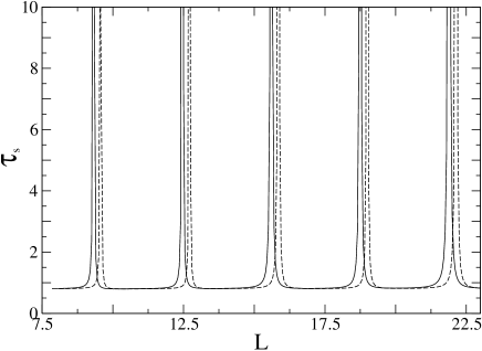
Figure 5: In absence of magnetic flux (i.e. $\phi$ =0 ), for a ring with two barriers of strength $V_{1}$ and $V_{3}$ separated by an intermediate well region, the saturated phase time $\tau_{s}$ is plotted as a function of ring’s circumference $L$ for different width $lb_{1}$ of the barrier. The solid and dashed curves are for $lb_{1}=2.75,3$ respectively. Other systems parameters are $lb_{2}=5$, $V_{1}=V_{3}=2$ and $E=1$.

IV CONCLUSIONS

We have generalized the Hartman effect beyond one dimension and in the presence of magnetic flux. This is done by studying the phase delay time in a circular geometric ring in the reflection mode. We have obtained an analytical expression for the saturated delay time. We have also shown that in the presence of successive opaque barriers separated by the potential well the saturated delay time becomes independent of the width of the well (in the long length limit) in the off resonant case. This is as if the effective velocity of the electron between the well becomes infinite or equivalently length of the well does not count (space collapse or space destroyer). We have further extended this effect in quantum mechanical networks with many arms wherein we have shown additional existence of new quantum non-local effects associated with the phase delay time mynew . Our reported results are amenable to experimental verifications for photon tunneling in appropriate electromagnetic geometries.

V Acknowledgments

One of the authors (SB) thanks Debasish Chaudhuri and Prof. Binayak Dutta-Roy for several useful discussions.

References

- (1) R. Landauer and T. Martin, Rev. Mod. Phys. 66 (1994) 217.
- (2) E. H. Hauge and J. A. Støvneng, Rev. Mod. Phys. 61 (1989) 917.
- (3) V. S. Olkhovsky and E. Recami, Physics Reports 214 (1992) 339.
- (4) S. Anantha Ramakrishna and N. Kumar, Europhys. Lett., 60 (2002) 491; Colin Benjamin and A. M. Jayannavar, Solid State Commun., 121 (2002) 591.
- (5) A. M Jayannavar, Pramana-journal of physics, 29 (1987) L341.
- (6) M. Büttiker, Pramana-journal of physics, 58 (2002) 241.
- (7) A. M. Steinberg, P. G. Kwiat, and R. Y. Chiao, Phys. Rev. Lett. 71 708 1993; R. Y. Chiao, P. G. Kwiat, and A. M. Steinberg, Scientific American, p. 38-46, August 1993.
- (8) A. Enders and G. Nimtz, J. Phys. I 2 (1992) 1693; 3 (1993) 1089; A. Enders and G. Nimtz, Phys. Rev. E, 48, 632 (1993); G. Nimtz, A. Enders and H. Spieker, ibid 4 (1994) 565.
- (9) P. Guerent, E. Marclay, and H. Meier, Solid State Commun. 68, 977 (1988); Ch. Spielmann, R. Szipocs, A. Sting, and F. Krausz, Phys. Rev. Lett. 73, 2308 (1994); Th. Hills et al., Phys. Rev. A 58, 4784 (1998).
- (10) H. G. Winful, Phys. Rev. Lett. 91 (2003) 260401; H. G. Winful, Phys. Rev. E68 (2003) 016615; H. G. Winful, Opt. Express 10 (2002) 1491.
- (11) V. S. Olkhovsky, E. Recami and G. Salesi, Europhys. Lett. 57 (2002) 879.
- (12) J. B. Xia, Phys. Rev. B45 (1992) 3593.
- (13) P. S. Deo and A. M. Jayannavar, Phys. Rev. B50 (1994) 11629.
- (14) S. Griffith, Trans. Faraday Soc. 49, 345 (1953) 650.
- (15) Y. Gefen, Y. Imry and M. Ya Azbel, Phys. Rev. Lett. 52 (1984) 129.
- (16) E. P. Wigner, Phys. Rev. 98 (1955) 145.
- (17) S. Washburn and R. A. Webb, Adv. Phys., 35 (1986) 375.
- (18) S. Datta, Electronic Transport in Mesoscopic Systems, Cambridge University Press, Cambridge, UK, 1997.
- (19) Swarnali Bandopadhyay, Raishma Krishnan, and A. M. Jayannavar, Solid State Commun. 131, 447 (2004); Swarnali Bandopadhyay and A. M. Jayannavar, Hartman effect and non-locality in quantum networks, quant-ph/0410126.