Electric circuit networks equivalent to chaotic quantum billiards

Abstract

We formulate two types of electric RLC resonance network equivalent to quantum billiards. In the network of inductors grounded by capacitors squared resonant frequencies are eigenvalues of the quantum billiard. In the network of capacitors grounded by inductors squared resonant frequencies are given by inverse eigen values of the billiard. In both cases local voltages play role of the wave function of the quantum billiard. However as different from quantum billiards there is a heat power because of resistance of the inductors. In the equivalent chaotic billiards we derive the distribution of the heat power which well describes numerical statistics.

I Introduction

Firstly electric circuit models representing a quantum particle in the one-dimensional potential

$$-\frac{\hbar^{2}}{2m}\frac{\partial^{2}\psi(x)}{\partial x^{2}}+V(x)\psi(x)=E\psi(x)$$ (1)

were considered by Kron in 1945 kron . Three types of equivalent circuits were established. The first one contains positive and negative resistors and in each state the currents and voltages are constant in time. The second and third models are similar and consist of inductors and capacitors and the currents and voltages are sinusoidal in time. Here we consider the stationary Schrödinger equation in two-dimensional billiards in hard wall approximation

$$-\nabla^{2}\psi(x,y)=\epsilon\psi(x,y),$$ (2)

where the Dirchlet boundary condition is implied at the boundary $C$ of the billiard:

$$\psi_{|{{}_{C}}}=0.$$ (3)

Here we use Cartesian coordinates $x,y$ which are dimensionless via a characteristic size of the billiard $L$, and correspondingly $\epsilon=\frac{E}{E_{0}},E_{0}=\frac{\hbar^{2}}{2mL^{2}}$.

There is a complete equivalence of the two-dimensional Schrödinger equation for a particle in a hard wall box to microwave billiards stockmann . A wave function is exactly corresponds to the the electric field component of the TM mode of electromagnetic field: $\psi(x,y)\leftrightarrow E_{z}(x,y)$ with the same Dirichlet boundary conditions. This equivalence is turned out very fruitful and allowed to test a mass of predictions found in the quantum mechanics of billiards stockmann . On the other hand, models for the equivalent RLC circuit of a resonant microwave cavity exist which establish the analogy near an eigenfrequency sucher . Manolache and Sandu manolache proposed a model of resonant cavity associated to an equivalent circuit consisting of an infinite set of coupled RLC oscillators. Therefore, there to be a bridge between quantum billiards and the set of coupled RLC oscillators berggren1 . In fact, we show here that at least, two models of electric resonance circuits (ERC) can be proposed. In the first model shown in Fig. 1 the eigen wave functions correspond correspond to voltages and eigen energies do to squared eigen frequencies of ERC. In the second model shown in Fig. 2 the eigen energies of quantum billiard correspond to the inverse squared eigen frequencies of the electric network. The electric network analogue systems allow to measure not only typically quantum variables such as probability and probability current distributions but also a distribution of heat power in chaotic billiards. Moreover intrinsic resistances of the RLC circuit allow to model the processes of decoherence.

II Electric resonance circuits equivalent to quantum billiards

If to map the two-dimensional Schrödinger equation onto numerical grid $(x,y)=a_{0}(i,j),i=1,2,\ldots N_{x},j=1,2,\ldots N_{y}$ one can easily obtain equation in finite element approximation

$$\psi_{i,j+1}+\psi_{i,j-1}+\psi_{i+1,j}+\psi_{i-1,j}+(a_{0}^{2}E-4)\psi_{i,j}=0.$$ (4)

The equivalent Hamiltonian is the tight-binding one

$$H=-\sum_{i,j}\sum_{{\bf b}}|ij\rangle\langle|ij+{\bf b}|,$$ (5)

where vector ${\bf b},|{\bf b}|=1$ runs over the nearest neighbors.

Let us consider the electric resonance circuit shown in Fig. 1. Each link of the two-dimensional network is given by the inductor L with the impedance

$$z_{L}=i\omega L+R$$ (6)

where $R$ is the resistance of the inductor and $\omega$ is the frequency. Each site of the network is grounded via the capacitor $C$ with the impedance

$$z_{C}=\frac{1}{i\omega C}.$$ (7)

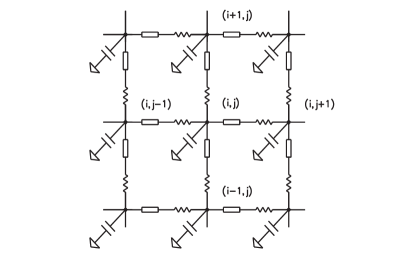
Figure 1: The first model of resonance RLC circuits.

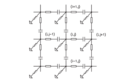
Figure 2: The second model of resonance RLC circuits.

The Kirchoff’s current law at each site of the network gives

$$\frac{1}{z_{L}}[V_{i,j+1}-V_{i,j}+V_{i,j-1}-V_{i,j}+V_{i+1,j}-V_{i,j}+V_{i-1,j}-V_{i,j}]-\frac{1}{z_{C}}V_{i,j}=0,$$ (8)

where $V_{i,j}$ are values of voltage at the site $(i,j)$. One can see that this equation coincides with the discretized version of the Schrödinger equation (4) with the eigenenergies as

$$a_{0}^{2}k^{2}=-\frac{z_{L}}{z_{C}}=LC\omega^{2}-iRC\omega=\frac{\omega^{2}}{\omega_{0}^{2}}-i\frac{\gamma\omega}{\omega_{0}^{2}},$$ (9)

where $\omega_{0}=1/\sqrt{LC}$ and $\gamma=R/L$ are the eigen frequency and the linewidth of each resonance circuit.

For the second network of electric resonance circuits shown in Fig. 2 we obtain

$$\frac{1}{z_{C}}[V_{i,j+1}-V_{i,j}+V_{i,j-1}-V_{i,j}+V_{i+1,j}-V_{i,j}+V_{i-1,j}-V_{i,j}]-\frac{1}{z_{L}}V_{i,j}=0.$$ (10)

Therefore, comparing with (4) we have

$$a_{0}^{2}k^{2}=-\frac{z_{C}}{z_{L}}=\frac{1}{LC\omega^{2}}+\frac{iR}{L\omega}=\frac{\omega_{0}^{2}}{\omega^{2}}+i\frac{\gamma\omega_{0}^{2}}{\omega}.$$ (11)

where $\gamma=RC$. This network is interesting in that its eigen frequencies are inverse to the eigenenergies of the quantum billiard.

There are many ways to define the boundary conditions (BC). Let it be $(i_{B},j_{B})$ are sites which belong to the boundary of the network. If these sites are grounded, we obtain obviously the Dirichlet BC (3) $V_{|_{B}}=0$. It they are shunted through capacitors we obtain the free BC (the von Neumann BC). At last, if the boundary sites are shunted through resistive inductors, the BC correspond to mixed BC.

III Analog of the chaotic Bunimovich billiard

A real electric circuit network has three features which can make a difference if to compare to the quantum billiards. These are 1) a discreteness of resonance circuits, 2) tolerance of electric elements, and 3) resistance of inductors. In practice the discreteness has no effect for $\lambda\geq 10a_{0}$ where $\lambda$ is a characteristic wavelength of wave function, and $a_{0}$ is the elementary unit of the network. Numerically we consider the electric network with shape as a quarter of the Bunimovich billiard. The distribution of real part of the wave function of the billiard mapped on the electric circuit network with $a_{0}=1/100$ is shown In Fig. 3 (a). The wavelength $\lambda=2\pi a_{0}\omega_{0}/\omega=0.115$ for parameters given in caption of Fig. 3. We take the width of the billiard as unit. One can see distinctive deviation from the Gaussian distribution which is result of multiple interference on discrete elements of the network.

It is known that a noise, for example, temperature, smoothes the conduction fluctuations for transmission through quantum billiards iida ; prigodin . In present case the tolerance of circuit elements, capacity and inductance, plays role of the noise. Therefore we can expect that increasing of the tolerance can suppress fluctuations of the distribution of the wave function of the discrete electric circuit network. In fact, even the $1\%$ tolerance substantially smoothes the distribution of the wave function as shown in Fig. 3 (b)-(d). We consider that the fluctuations of capacitors and inductors are not correlated at different sites.

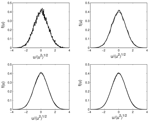
Figure 3: The distribution of real part of the wave function of the quarter Bunimovich billiard mapped on resonance RLC circuit with elementary unit $a_{0}=0.01,\omega=1.722MHz,L=0.1~{}mH,C=1~{}nF,R=0$. (a) There is no tolerance of the electric circuit elements. (b) The tolerance equals to $1\%$. (c) The tolerance equals to $3\%$. (d) The tolerance equals to $5\%$. Each distribution in (b) - (d) is averaged over 100 realizations of the electric network.

Finally we consider as a damping caused by resistance of the inductors effects the distribution of the wave function in the electric RLC resonance circuit network. In order to excite the network we apply external ac current at single site of the network. Fig. 4 shows the probability density in the quarter of the Bunimovich billiard for two values of the resistance $R$. One can see from Fig. 4 (right) a localization effect because of a damping of the probability density flowing from ac source (see also Fig. 7). The characteristic length of space damping can be easily estimated from Eq. (9) which gives us

$$\lambda_{R}\approx\frac{4\pi a_{0}}{R}\sqrt{\frac{L}{C}}.$$ (12)

The distributions of the probability density $\rho=|V|^{2}$ for open quantum chaotic billiards were considered in many articles lenz ; lenz1 ; kanzieper ; pnini ; ishio for the case of zero damping. Here we follow saichev ; ishio and perform the phase transformation $V\rightarrow V\exp(i\theta)=p+iq$ which makes the real and imaginary parts of the wave function $V$ independent. Introducing a parameter of openness of the billiard saichev

$$\epsilon^{2}=\frac{\sigma_{q}^{2}}{\sigma_{p}^{2}}.$$ (13)

where $\sigma_{p}^{2}=\langle p^{2}\rangle,~{}\sigma_{q}^{2}=\langle q^{2}\rangle$ we can write the distribution of probability density as ishio

$$f(\rho)=\mu\exp(-\mu^{2}\rho)I_{0}(\mu\nu\rho),$$ (14)

with the following notations

$$\mu=\frac{1}{2}\left(\frac{1}{\epsilon}+\epsilon\right),\nu=\frac{1}{2}\left(\frac{1}{\epsilon}-\epsilon\right),$$ (15)

and $I_{0}(x)$ is the modified Bessel function of zeroth order, This distribution is shown in Fig. 5 by solid lines while the Rayleigh distribution $f(\rho)=\exp(-\rho)$ is shown by dashed lines. The Rayleigh distribution specifies the distribution of completely open system. One can see from Fig. 5 (a, b) that the statistics of the probability density follows the distribution (14) irrespective to resistance $R$. However with growth of the resistance the distribution (14) tends to the Rayleigh distribution (Fig. 5 (c, d)). Since the larger resistance the more quantum system is open, this tendency of statistics of the probability density is clear.

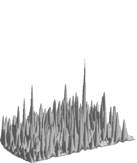
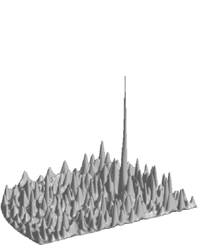
Figure 4: Views of probability density of the quarter Bunimovich billiard mapped on resonance RLC circuit with elementary unit $a_{0}=0.005$, $\omega=0.8611~{}MHz,L=0.1~{}mH,C=1~{}nF$. Left $R=0.5~{}\Omega$, right $R=1~{}\Omega$. The point of connection of external ac current is at maximum of the probability density.

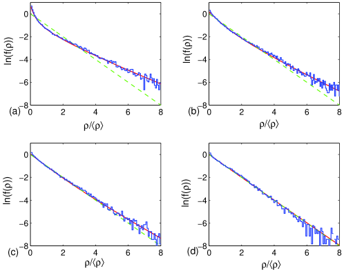
Figure 5: (Color online) Distribution of probability density of the quarter Bunimovich billiard mapped on resonance RLC circuit with the same parameters as given in Fig. 4. (a) $R=0.1~{}\Omega,Q=3162,\epsilon=0.2488$, (b) $R=0.3~{}\Omega,Q=1054,\epsilon=0.5308$, (c) $R=0.5~{}\Omega,Q=632,\epsilon=0.6996$ and (d) $R=1~{}\Omega,Q=316,\epsilon=0.9164$. The distribution (14) is shown by solid red line, the Rayleigh distribution $f(\rho)=\exp(-\rho)$ is shown by dashed green line.

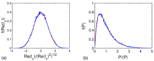
Figure 6: (Color online) (a) Statistics of the real part of the x-component of electric current $I_{x}$ compared to the Gaussian distribution shown by solid red line. (b) Statistics of the heat power compared to the distribution 28 shown by solid red line. Here the quarter Bunimovich billiard is taken with $\omega=1.163~{}MHz,R=0.1~{}\Omega,L=0.1~{}mH,C=1~{}nF$.

IV The heat power

In open systems the probability current density corresponds to the Poynting vector. The last equivalence allowed to test in particular universal current statistics in chaotic billiards barth ; saichev . However in the electric resonance circuit there is the heat losses because of the resistance. A local power of the heat losses is defined by formula heat

$$P=\frac{R}{2}[Re(I_{x})^{2}+Im(I_{x})^{2}+Re(I_{y})^{2}+Im(I_{y})^{2}]=\frac{R}{2}[|I_{x}|^{2}+|I_{y}|^{2}],$$ (16)

where $I_{x},I_{y}$ are local components of the electric power flowing between sites of the electric network:

$$RI_{x}(i,j)=V_{i+1,j}-V_{i,j},\quad RI_{y}(i,j)=V_{i,j+1}-V_{i,j}.$$ (17)

If to approximate the true state with the Berry conjecture

$$V(x,y)=\sum_{j}a_{j}\exp[i~{}({\bf k_{j}r}+\phi_{j})]$$ (18)

where $a_{j}$ and $\phi_{j}$ are independent random real variables and $k_{j}$ are randomly oriented wave vectors of equal length, then $V$ is the complex random Gaussian field (RGF) in the chaotic Bunimovich billiard. The derivatives of $V$ are also independent complex RGFs. The components $I_{x},~{}I_{y}$ form two complex RGFs with the probability density of these fields

$$f(I_{x}^{\prime},I_{y}^{\prime},I_{x}^{\prime\prime},I_{y}^{\prime\prime})=\frac{1}{4\pi^{2}\sigma_{r}^{2}\sigma_{i}^{2}}\exp\left\{-\frac{1}{2}\left(\frac{I_{x}^{\prime 2}+I_{y}^{\prime 2}}{\sigma_{r}^{2}}+\frac{I_{x}^{\prime\prime 2}+I_{y}^{\prime\prime 2}}{\sigma_{i}^{2}}\right)\right\}$$ (19)

where $I_{x}^{\prime}=Re(I_{x}),~{}I_{y}^{\prime}=Re(I_{y}),~{}I_{x}^{\prime\prime}=Im(I_{x}),~{}I_{y}^{\prime\prime}=Re(I_{y}),~{}\sigma_{r}^{2}=\langle I_{x}^{\prime 2}\rangle,\langle I_{y}^{\prime 2}\rangle,~{}\sigma_{i}^{2}=\langle I_{x}^{\prime\prime 2}\rangle,\langle I_{y}^{\prime\prime 2}\rangle$. In numerical computations we use that average over the billiard area

$$\langle\ldots\rangle=\frac{1}{A}\int d^{2}{\bf x}\ldots,$$ (20)

is equivalent to average over three complex GRFs

$$\langle\ldots\rangle=\int d^{2}Vd^{2}I_{x}d^{2}I_{y}f(Re(V),Im(V))f(I_{x}^{\prime},I_{y}^{\prime},I_{x}^{\prime\prime},I_{y}^{\prime\prime})\ldots.$$ (21)

An example of the distribution of the real part of $I_{x}$ is presented in Fig. 6 (a) which shows that numerically this value is, in fact, the RGF. A definition of the probability distribution (19) is relied on that the Berry function (18) is isotropic in space : $\langle I_{x}^{\prime 2}\rangle=\langle I_{y}^{\prime 2}\rangle,~{}\langle I_{x}^{\prime\prime 2}\rangle=\langle I_{y}^{\prime\prime 2}\rangle$. In fact, an anisotropy of the shape of billiard effects an anisotropy. However this effect is the boundary condition’s one which has of order $L_{P}\lambda/A\sim\lambda$, where $L_{P}$ is a length of the billiard perimeter, and $\lambda$ is a characteristic wave length of wave function in terms of the width of the billiard. Therefore, for the excitation of the eigenfunction with sufficiently high frequency we can use the distribution function (19). Table 1 of numerically computed mean values confirms this conclusion.
 
Table 1. Numerically computed mean values.
 
$\omega$, MHz the wavelength $\lambda$ in terms of the billiard’s width $\frac{\langle I_{x}^{\prime 2}\rangle-\langle I_{y}^{\prime 2}\rangle}{\langle I_{x}^{\prime 2}\rangle+\langle I_{y}^{\prime 2}\rangle}$ $\frac{\langle I_{x}^{\prime\prime 2}\rangle-\langle I_{y}^{\prime\prime 2}\rangle}{\langle I_{x}^{\prime\prime 2}\rangle+\langle I_{y}^{\prime\prime 2}\rangle}$ $\epsilon$ 0.8611 0.1154 0.095 -0.128 0.2488 1.1623 0.0854 0.056 0.050 $0.6103$
 

To find the distribution of the heat power (16) it is convenient to begin with a characteristic function

$$\Theta(a)=\langle\exp(iaP)\rangle=\int d^{2}I_{x}d^{2}I_{y}f(I_{x}^{\prime},I_{y}^{\prime},I_{x}^{\prime\prime},I_{y}^{\prime\prime})\exp(iaR[|I_{x}|^{2}+|I_{y}|^{2}]/2).$$ (22)

Substituting (19) we obtain

$$\Theta(a)=-\frac{(\sigma_{r}^{2}+\sigma_{i}^{2})^{2}}{\sigma_{r}^{2}\sigma_{i}^{2}}\frac{1}{\left(a+i\frac{\sigma_{r}^{2}+\sigma_{i}^{2}}{\sigma_{r}^{2}}\right)\left(a+i\frac{\sigma_{r}^{2}+\sigma_{i}^{2}}{\sigma_{i}^{2}}\right)}.$$ (23)

A knowledge of the characteristic function allows to find the heat power distribution function

$$f(P)=\frac{1}{2\pi}\int_{-\infty}^{\infty}da\Theta(a)\exp(-iaP)=\frac{2\mu}{\nu\langle P\rangle}\exp(-\mu P/\langle P\rangle)\sinh(\nu P/\langle P\rangle),$$ (24)

where formulas (15 take the following form

$$\mu=\frac{(\sigma_{r}^{2}+\sigma_{i}^{2})^{2}}{2\sigma_{r}^{2}\sigma_{i}^{2}},\quad\nu=\frac{(\sigma_{r}^{2}-\sigma_{i}^{2})^{2}}{2\sigma_{r}^{2}\sigma_{i}^{2}}.$$ (25)

For $\sigma_{r}^{2}\approx\sigma_{i}^{2}$ the distribution takes the very simple form

$$f(P)=\frac{4P}{\langle P\rangle^{2}}\exp(-2P/\langle P\rangle),$$ (26)

Even for this case the distribution of heat power differs from the distribution of the probability current saichev . The parameter of openness of the billiard (13) can be approximated as

$$\epsilon^{2}=\frac{\sigma_{i}^{2}}{\sigma_{r}^{2}}.$$ (27)

It is easy to obtain from the Schrödinger equation that $2\sigma_{r}^{2}=E\sigma_{p}^{2},~{}2\sigma_{i}^{2}=E\sigma_{q}^{2}$ from which the last equality in (27) follows.

Then the heat power distribution function (24) can be written as follows

$$f(P)=\frac{1+\epsilon^{2}}{1-\epsilon^{2}}\left\{\exp\left(-\frac{(1+\epsilon^{2})P}{\langle P\rangle}\right)-\exp\left(-\frac{(1+\epsilon^{2})P}{\epsilon^{2}\langle P\rangle}\right)\right\}.$$ (28)

This distribution is shown in Fig. 6 (b) which as one can see nicely describes numerically computed statistics of the heat power. If to introduce a value

$$\sigma_{P}^{2}=\frac{\langle(P-\langle P\rangle)^{2}\rangle}{\langle P\rangle^{2}},$$ (29)

then one can derive the relation between this parameter and the parameter of openness (27)

$$\sigma_{P}^{2}=\frac{\epsilon^{4}+1}{(\epsilon^{2}+1)^{2}}.$$ (30)

If the quantum system is fully opened, $\epsilon=1$, and we have from (30) that $\sigma_{P}^{2}=1/2$. For the limit of closed quatum system we obtain correspondingly that $\sigma_{P}^{2}=1$.

V summary and conclusions

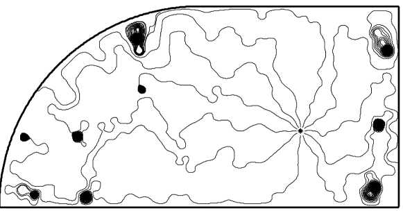
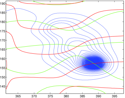
Figure 7: Top: quantum streamlines in the quarter of the Bunimovich billiard flowing from point shown by star at which the external ac current is applied. (Color online) Bottom: zoomed part of top figure. Blue lines show the streamline, red and green lines are the nodal lines of the real and imaginary parts of wave function correspondingly. The points at which the nodal lines intersecting are centers of the vortices berggren . The wave function corresponds to Fig. 4 (right) with the same parameters.

We established two types of the electric circuit networks of the RLC resonant oscillators in which voltages play role of quantum wave function. Specifically we considered the electric networks with the Dirichlet boundary conditions which are equivalent to the quarter of the Bunimovich quantum billiard. In fact, the electric circuit network has three features which can make a difference if to compare with the quantum billiards. These are a discreteness of resonance circuits, tolerance of electric elements, and resistance of inductors. We showed numerically that the first two features are conceal each other. The resistance of the electric network gives rise to a heat which can be described locally by the heat currents. Assuming that the wave function in the billiard can be given as the complex random Gaussian field we derived the distribution of the heat power which well describe numerical statistics.

The third feature of the electric network, resistance has principal importance. The resistance of the electric network is originated from inelastic interactions of electrons with phonons and other electrons which give rise to irreversible processes of decoherence. With growth of the resistance the wave function is becoming localized. We studied as the probability density and the probability currents evolves with increasing of the resistance. Therefore we can conclude that the resistance violates the equation $\nabla{\bf j}=0$. In fact Fig. 7 demonstrates unusual behavior of quantum streamlines berggren with growth of the resistance. One can see that the quantum streamline are terminating at the vortex cores. The vortices serve as sinks for the probability density shown in Fig. 7 (top) as spots. Therefore the resistance of the inductors in the equivalent electric networks is simple mechanism of a deterioration of ballistic transport similar to the Büttiker mechanism buttiker .

- (1) G. Kron, Phys. Rev. 67, 39 (1945).
- (2) H.-J. Stöckmann, Quantum Chaos: An Introduction (Cambridge University Press, Cambridge, UK, 1999).
- (3) Handbook of Microwave Measurements, edited by M. Sucher and J. Fox (Polytechical Press, New York, 1963).
- (4) F. Manolache and D.D. Sandu, Phys. Rev. A49, 2318 (1994).
- (5) K.-F. Berggren and A.F Sadreev, Chaos in quantum billiards and similarities with pure-tone random models in acoustics, microwave cavities and electric networks, Proc. of Vajxo Conf. in ”Foundations of Probability”, (2003).
- (6) S.Iida, H.A.Weidenmüller, and J.A.Zuk, Phys. Rev. Lett. 64, 583 (1990).
- (7) V.N.Prigodin, K.B.Efetov, and S.Iida, Phys. Rev. Lett. 71, 1230 (1993).
- (8) K. Życzkowski and G. Lenz, Z. Phys. B: Condens. Matter 82, 299 (1991).
- (9) G. Lenz and K. Życzkowski, J. Phys. A 25, 5539 (1992).
- (10) E. Kanzieper and V. Freilikher, Phys. Rev. B 54, 8737 (1996).
- (11) R. Pnini and B. Shapiro, Phys. Rev. E 54, R1032 (1996).
- (12) H. Ishio, A.I. Saichev, A.F. Sadreev,and K.-F. Berggren, Phys. Rev. E64, 056208 (2001).
- (13) M. Barth and H.-J. Stöckmann, Phys. Rev. E 65, 066208 (2002).
- (14) A.I.Saichev, H.Ishio, A.F.Sadreev, and K.-F.Berggren, J. Phys. A: Math. and General,35, L87 (2002).
- (15) B.D. Popovic, Introductory engineering electromagnetics, Addison-Wesley, 1971.
- (16) A.F.Sadreev and K.-F. Berggren, Phys. Rev. E 70, 026201 (2004).
- (17) K-F. Berggren, A. F. Sadreev, and A.A. Starikov, Phys. Rev. E66, 016218 (2002).
- (18) M. Büttiker, Phys. Rev. B33, 3020 (1986).