Efficient decoupling and recoupling in solid state NMR for quantum computation

Abstract

A scheme for decoupling and selectively recoupling large networks of dipolar-coupled spins is proposed. The scheme relies on a combination of broadband, decoupling pulse sequences applied to all the nuclear spins with a band-selective pulse sequence for single spin rotations or recoupling. The evolution-time overhead required for selective coupling is independent of the number of spins, subject to time-scale constraints, for which we discuss the feasibility. This scheme may improve the scalability of solid-state-NMR quantum computing architectures.

I Introduction

Nuclear spins have been proposed as quantum bits (qubits) for quantum computation, due to their good isolation from the environment.Gershenfeld and Chuang (1997); Cory et al. (1997) With the aid of the established technology of nuclear magnetic resonance (NMR) and the use of “pseudo-pure” states,Gershenfeld and Chuang (1997); Cory et al. (1997); Knill et al. (1998) liquid NMR at room temperature has allowed the largest quantum computers to date.Vandersypen et al. (2001)

In liquid NMR, a solution is used in which each solute molecule has several nuclei, each nucleus having a different Larmor frequency in the presence of a magnetic field. This allows selective addressing of the nuclei through application of resonant radio-frequency (RF) fields at the corresponding frequencies. Each synthesized molecule in the aqueous solution undergoes the same logic operations.

Within each molecule, logic operations are performed by successive application of single-bit rotations (by RF pulse sequences) and multi-qubit conditional operations (by time-evolution in the presence of coupling among the qubits). The design of such logic gates relies on the assumption that the coupling among the specific qubits can be set at will to on (coupled) for construction of a logic gate, and off (decoupled) for absence of a logic gate. A systematic scheme for this has been developed,Leung et al. (2000) but requires sequences of duration $O(n)$ as the number of qubits $n$ increases, resulting in a clock-speed that decreases as the computer-size increases.Lad Because this slow-down is only linear in $n$, and because some quantum algorithms afford exponential speed-up, the scheme is efficient in principle. However, truly scalable operation will require quantum fault tolerance,Nielsen and Chuang (2000) which requires logic gates to be sufficiently accurate and fast in comparison to decoherence times to surpass the fault-tolerance threshold. Faster logic gates are therefore of crucial importance for future NMR quantum computers.

As an alternative to a liquid, the use of dipolar-coupled nuclear spins in a crystalline solid Yamaguchi and Yamamoto (1999); Ladd et al. (2002) possesses certain merits for scalability, such as long coherence times,Ladd et al. (2004) the ability to polarize the nuclear spins by optical pumping of electron spins,Verhulst et al. (2004) and more sensitive methods of nuclear-spin detection.Ladd et al. (2002); Fu et al. (2004) However, it introduces additional complexity to the design of the pulse sequences needed for logic operations. In these proposed schemes, a magnetic field gradient is introduced to differentiate qubit ensembles, by analogy to the chemical shift in liquid-NMR. Unlike liquid-NMR, however, nuclei within a single qubit ensemble are dipole-coupled. The complexity of pulse sequence design arises from the additional burden of constantly decoupling these intra-ensemble nuclear spins, which have the same Larmor frequency, while also decoupling and recoupling nuclear spins with distinct Larmor frequencies.

In this article, we propose a scheme that addresses both of these issues: the linear slowing of logic operations and the complication of added couplings in a crystalline state. The required ingredients are that all spins must be coupled by strictly dipolar (or pseudo-dipolar) couplings in a large magnetic field, the field gradient or chemical shift distinguishing these qubits must be very large, and the couplings between different qubits must be much stronger than couplings within an ensemble. As previously discussed,Ladd et al. (2002) this last condition may be achieved in a geometry where nuclei are placed in one-dimensional atomic chains, with a field gradient parallel to the chains. Multiple, well-separated chains form the weakly coupled ensemble. Other geometries, such as well-separated ensembles of planar monolayers with two-dimensional gradients,Goldman et al. (2000) are possible as well.

II Description of the Spin System

In the presence of a static magnetic field along the $z$-axis, the Hamiltonian consists of the Zeeman energy of the nuclear spins and the coupling between nuclear spins by the dipole-dipole interaction. The Zeeman term is written

$$H_{\rm Z}=-\gamma\hbar\sum_{k}B_{k}^{\phantom{z}}I_{k}^{z}=-\sum_{k}\hbar\omega_{k}^{\phantom{z}}I_{k}^{z},$$ (1)

where $\gamma$ is the gyromagnetic ratio of the nuclear spin and $B_{k}$ is the magnetic field at the location of nuclear spin $k$. Due to the field gradient, the magnetic fields $B_{k}$ and therefore the Larmor frequencies $\omega_{k}$’s of the nuclear spins differ. We denote the gradient-induced resonant frequency separation between adjacent nuclei as $\omega_{k+1}-\omega_{k}=\delta\omega.$ The average Larmor frequency, which we notate $\omega_{0}$, is much faster than all other frequencies in the system.

The dipole-dipole interaction between two nuclear spins $k$ and $l$ separated by the vector ${\bf r}_{kl}$ is given by,Abragam (1961)

$$H_{\rm D}=\frac{\mu_{0}}{4\pi}\frac{\hbar^{2}\gamma^{2}}{r_{kl}^{3}}\left\{{\bf I}_{k}\cdot{\bf I}_{l}-3\frac{({\bf I}_{k}\cdot{\bf r}_{kl})({\bf I}_{l}\cdot{\bf r}_{kl})}{r_{kl}^{2}}\right\}.$$ (2)

In the presence of a large applied field, the terms similar to $I_{k}^{z}I_{l}^{x}$ or $I_{k}^{x}I_{l}^{y}$ oscillate at frequencies near $\omega_{0}$ or $2\omega_{0}$, respectively. These nonsecular terms contribute negligibly to the evolution in the timescale under consideration.Abragam (1961) With this approximation, the dipole coupling for a pair of nuclear spins $k$ and $l$ takes the form

$$H_{\rm D}^{z}=D_{kl}^{\phantom{z}}\left(2I^{z}_{k}I^{z}_{l}-I^{x}_{k}I^{x}_{l}-I^{y}_{k}I^{y}_{l}\right),$$ (3)

where

$$D_{kl}=\frac{\mu_{0}}{4\pi}\gamma^{2}\hbar^{2}\frac{1-3\cos^{2}\theta_{kl}}{2r_{kl}^{3}},$$ (4)

and $\theta_{kl}$ is the angle between ${\bf r}_{kl}$ and the $z$-axis. The dipole coupling strength $D_{kl}$ between neighboring nuclei is typically several hundred hertz, but can be smaller depending on the geometry of the system.

The nuclear spins are manipulated by an oscillating RF magnetic field $B_{1}$ in the plane perpendicular to the $z$-axis. In the following, a “broadband” pulse (or “hard” pulse) with Rabi frequency $\gamma B_{1}=\Omega_{\rm RF}$ has a pulse duration $\sim 1/\Omega_{\rm RF}$ much smaller than $1/n\delta\omega$. A “selective” pulse (or “soft” pulse) with Rabi frequency $\omega_{\rm RF}$ has a pulse duration much longer than $1/\delta\omega$ in order to selectively rotate spins of a single Larmor frequency $\omega_{k}$. Nearest-neighbor spins receive an erroneous rotation of order $\text{sinc}(\pi\delta\omega/2\omega_{\rm RF})$; these erroneous rotations can be corrected by pulse shaping techniques discussed elsewhere.Steffen et al. (2000)

The couplings between nuclear spins and “broadband” and “selective” RF fields neglecting counter-rotating componentsAbragam (1961) are described by the Hamiltonians

$$H_{\rm RF}^{\rm B} =-\hbar\Omega_{\rm RF}\sum_{k}\left[\cos(\omega t-\phi)I_{k}^{x}-\sin(\omega t-\phi)I_{k}^{y}\right],$$ (5)

$$H_{\rm RF}^{\rm S} =-\sum_{l,k}\hbar\omega_{\rm RF}^{l}\left[\cos(\omega^{\prime}_{l}t-\phi_{l})I_{k}^{x}-\sin(\omega^{\prime}_{l}t-\phi_{l})I_{k}^{y}\right],$$ (6)

for broadband (B) and selective (S) pulses, where $I_{k}^{\pm}=I_{k}^{x}\pm iI_{k}^{y}$. We denote the angular frequencies and phases as $\omega$ and $\phi$ for a broadband pulse and $\omega^{\prime}_{l}$ and $\phi_{l}$ for a selective pulse targeted on spin $l$.

When broadband pulses are applied, their time scale is $1/n\delta\omega\ll 1/\delta\omega$. Thus the dipole coupling between any pair of nuclear spins is well described by Eq. (3). For simplicity, perfect delta-pulses are assumed for broadband pulses; each pulse can be applied instantaneously. In practice, the effect of finite pulse widths due to limited RF power in a real NMR experimentSteffen et al. (2000) needs to be considered and accommodated before the proposed scheme is implemented. We make a further assumption requiring greater scrutiny: we assume that selective pulses can be performed quickly in comparison to the free dipolar dynamics, thus allowing selective pulses that appear as $\delta$-functions with respect to averages of the dipolar Hamiltonian. This requires that $\delta\omega\gg D_{kl}$. The applicability of these assumptions will be discussed in Sec. IV.

III Scheme for Decoupling and Recoupling

III.1 Broadband decoupling

To establish our formalism for analyzing decoupling pulse sequences, we summarize the celebrated multiple-pulse sequence for decoupling, commonly called WHH-4 (or WAHUHA) Waugh et al. (1968).

We begin by considering the effect of a broadband pulse on the spins in the absence of selective pulses. We consider the usual “rotating reference frame,” which rotates at the $RF$ frequency $\omega$. In this frame the spins undergo a time evolution governed by the total Hamiltonian $H_{\rm Z}+H_{\rm RF}^{\rm B}+H_{\rm D}^{z}$, written in the form

$$H=-\sum_{k}\hbar\delta\omega_{k}I_{k}^{z}-\frac{\hbar\Omega_{\rm RF}}{2}\sum_{k}\left[e^{-i\phi}I_{k}^{+}+e^{i\phi}I_{k}^{-}\right]+H_{\rm D}^{z},$$ (7)

where $\delta\omega_{k}=\omega_{k}-\omega$. Since $\Omega_{\rm RF}\gg|\delta\omega_{k}|\gg D_{kl}$, the broadband pulse causes a rotation about the unit vector $\hat{n}=[\cos\phi,\sin\phi,0]$ by angle $\theta=\Omega_{\rm RF}t$ a rotation we consider as instantaneous. The unitary operator for such a rotation is $P_{\phi}=\exp(-i\theta I^{\phi})$. The dipolar-decoupling sequence WHH-4 consists of four such broadband pulses, all with $\theta=\pi/2$. For this sequence we notate such a pulsed rotation with $\phi=0$ as $P_{x}$, with $\phi=\pi/2$ as $P_{y}$, etc.

To understand the evolution of the spins during a fast sequence of such pulses, we transform our Hamiltonian to a reference frame that follows the pulses. This reference frame is referred to as the “toggling frame.” A Hamiltonian $H$ written in this frame will be denoted $\tilde{H}(t)$. If there were no dipolar evolution or field gradient, then spins in the toggling frame would undergo no evolution whatsoever, even though the $P_{\alpha}$ pulses are causing rapid revolutions in the rotating frame. Toggling-frame dynamics can be observed by “stroboscopic” observation, in which measurement with a particular phase reference is performed only once per cycle, when the toggling frame coincides with the rotating frame.

At the beginning of a cycle, the dipole coupling Hamiltonian of Eq. (3) in the toggling frame coincides with $H_{\rm D}^{z}$;

$$\tilde{H}_{\rm D}(0<t<\tau)=H_{\rm D}^{z}.$$ (8)

When we apply a $P_{x}$ pulse at $t=\tau$ and a $P_{\bar{y}}$ pulse at $t=2\tau$, then the toggling frame Hamiltonian becomes

$$\tilde{H}_{\rm D}(\tau<t<2\tau)=P_{\bar{x}}H_{\rm D}^{z}P_{x}\\ =D_{kl}(2I_{k}^{y}I_{l}^{y}-I_{k}^{x}I_{l}^{x}-I_{k}^{z}I_{l}^{z})\equiv H_{\rm D}^{y},$$ (9)

and

$$\tilde{H}_{\rm D}(2\tau<t<3\tau)=P_{\bar{x}}P_{y}H_{\rm D}^{z}P_{\bar{y}}P_{x}=H_{\rm D}^{x}.$$ (10)

Similarly, a $P_{y}$ pulse at $t=4\tau$ returns the toggling frame Hamiltonian to

$$\tilde{H}_{\rm D}(4\tau<t<5\tau)=P_{\bar{x}}P_{y}P_{\bar{y}}H_{\rm D}^{z}P_{y}P_{\bar{y}}P_{x}=H_{\rm D}^{y}.$$ (11)

Finally a $P_{\bar{y}}$ pulse at $t=5\tau$ brings the toggling frame Hamiltonian back to $H_{\rm D}^{z}$;

$$\tilde{H}_{\rm D}(5\tau<t<6\tau)=P_{\bar{x}}P_{y}P_{\bar{y}}P_{y}H_{\rm D}^{z}P_{\bar{y}}P_{y}P_{\bar{y}}P_{x}=H_{\rm D}^{z}.$$ (12)

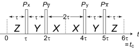
Figure 1: Decoupling pulse sequence WHH-4. Mehring (1983) $\bm{P}_{\alpha}$ and $\bm{P}_{\bar{\alpha}}$ stand for $\pi/2$ and $-\pi/2$ pulses around the $\alpha$-axis ($\alpha=x,y$). The system whose Hamiltonian is $H$ evolves in the toggling frame by $Z=H$ for time 2$\tau$, $Y=P_{\bar{x}}HP_{x}$ for time 2$\tau$ and $X=P_{\bar{x}}P_{y}HP_{\bar{y}}P_{x}$ for time 2$\tau$ in one cycle $t_{c}=6\tau$. In the case of the dipole coupling Hamiltonian of Eq. (3), the zero-order term and all odd-order terms in the average Hamiltonian vanish over the period $t_{c}$.

The decoupling pulse sequence WHH-4 shown in Fig. 1 is designed so that the system evolves in the toggling frame by ${H}_{\rm D}^{x}$ for time $2\tau$, ${H}_{\rm D}^{y}$ for time $2\tau$ and $H_{\rm D}^{z}$ for time $2\tau$ in one cycle. The total cycle time $t_{c}$ is $6\tau$.

We see that this particular WHH-4 cycle of form

$$\tau,P_{x},\tau,P_{\bar{y}},2\tau,P_{y},\tau,P_{\bar{x}},\tau$$

causes a spin operator $I^{z}_{j}$ in the rotating-frame Hamiltonian to go to $I^{y}_{j}$, then to $I^{x}_{j}$, and then back again, in the toggling-frame Hamiltonian. We therefore notate this cycle as $[\![Z,Y,X]\!]$ following the notation of MansfieldMansfield (1971). Several equivalent WHH-4 sequences exist. For example, if $P_{x}$ is replaced by $P_{\bar{x}}$ to make the sequence $\tau,P_{\bar{x}},\tau,P_{\bar{y}},2\tau,P_{y},\tau,P_{x},\tau$, then we would find $I^{z}$ going to $-I^{x}$, to $I^{y}$, and then back again, and so we notate this cycle as $[\![Z,\bar{Y},X]\!]$.

In average Hamiltonian theory (AHT), the unitary evolution in the toggling frame under this changing Hamiltonian is calculated by a time ordered exponential, expanded via the Magnus expansionMehring (1983). The zero-order term is simply the average Hamiltonian over the period of the sequence ${t_{\rm c}}$:

$$\bar{H}=\frac{1}{t_{\rm c}}\int_{0}^{t_{\rm c}}\tilde{H}(t)dt.$$ (13)

For any WHH-4 sequence, the average Hamiltonian for the dipole coupling is

$$\bar{H}_{\rm D}=\frac{1}{6\tau}(2\tau H_{\rm D}^{x}+2\tau H_{\rm D}^{y}+2\tau H_{\rm D}^{z})=0.$$ (14)

It may be shown that all odd-order dipolar terms of the average Hamiltonian vanish as well, due to the symmetry of the cycle.Mehring (1983)

It is important to realize that dipolar-decoupling sequences have been heavily developed in NMR over the past 40 years. By compounding these sequences with super-cycles, they can be made robust against finite pulse width, pulse errors, and higher order terms in AHT. More modern sequences such as BR-24Burum and Rhim (1979) and CORY-48Cory et al. (1990) have routinely proven their effectiveness in reducing the timescale for dipolar evolution by three or more orders of magnitude.

Among such pulse sequences is MREV-16, a variation of MREV-8P. Mansfield and Richards (1973); W-K. Rhim and Vaughan (1973), one cycle of which is expressed as $[\![Z,Y,X]\!][\![Z,\bar{Y},X]\!][\![Z,Y,\bar{X}]\!][\![Z,\bar{Y},\bar{X}]\!].$ The cycle time is $t_{c}=24\tau$. This sequence is more robust against pulse imperfections than WHH-4, but it also contains an additional advantage. The simple sequence $[\![Z,Y,X]\!]$ averages offset terms proportional to $I_{k}^{z}$, $I_{k}^{x}$ and $I_{k}^{y}$ to

$$\bar{I}_{k}^{z}=\frac{I_{k}^{x}+I_{k}^{y}+I_{k}^{z}}{3},\ \ \bar{I}_{k}^{x}=\frac{2I_{k}^{x}-I_{k}^{y}}{3},\ \ \bar{I}_{k}^{y}=\frac{I_{k}^{y}-2I_{k}^{z}}{3},$$ (15)

while the compound sequence MREV-16 yields the average operators

$$\bar{I}_{k}^{z}=\frac{1}{3}{I}_{k}^{z},\qquad\bar{I}_{k}^{x}=\frac{2}{3}{I}_{k}^{x},\qquad\bar{I}_{k}^{y}=\frac{1}{3}{I}_{k}^{y}.$$ (16)

In the case of MREV-16, $\bar{I}_{k}^{x}$ and $\bar{I}_{k}^{y}$ lie in the plane perpendicular to $\bar{I}_{k}^{z}$, while this is not the case for any WHH-4 sequence. This property is critical for allowing selective RF rotations during decoupling, as we discuss in the following section.

III.2 Selective rotations

Application of MREV-16 during selective pulses

We now show how to produce selective spin rotations on desired spins while decoupling the dipole coupling between them by the MREV-16 broadband decoupling pulse sequence. The result of such a selective RF pulse is to affect the evolution of the desired spin ensemble, while leaving all other spins unaffected.

Suppose we weakly irradiate the spins by selective pulses as in Eq. (6), while simultaneously applying the broadband decoupling sequence MREV-16. The RF Hamiltonian for selective pulses Eq. (6) is written as

$$H_{\rm RF}^{\rm S}=-\sum_{l}\frac{\hbar\omega_{\rm RF}^{l}}{2}\sum_{k}\left[e^{-i(\delta\omega^{\prime}_{l}t+\phi_{l})}I_{k}^{+}+e^{i(\delta\omega^{\prime}_{l}t+\phi_{l})}I_{k}^{-}\right],$$ (17)

in the rotating frame at the angular frequency $\omega$ of the broadband pulses, where $\delta\omega^{\prime}_{l}=\omega^{\prime}_{l}-\omega$. Since $\Omega_{\rm RF}\gg|\delta\omega_{l}|$, Eq. (17) varies slowly in time as compared to durations and intervals of fast broadband pulses in the decoupling sequence. Therefore, $H_{\rm RF}^{\rm S}$ is averaged by MREV-16 as if Eq. (17) were time-independent;

$$\bar{H}_{\rm RF}^{\rm S}=-\sum_{l}\frac{\hbar\omega_{\rm RF}^{l}}{2}\sum_{k}\left[e^{-i(\delta\omega^{\prime}_{l}t+\phi_{l})}\frac{3I_{k}^{+}+I_{k}^{-}}{6}+{\rm h.c.}\right].$$ (18)

Here we have made use of the fact that $I_{k}^{+}=I_{k}^{x}+iI_{k}^{y}$ is averaged to $(3I_{k}^{+}+I_{k}^{-})/6$ by MREV-16.

We next show that this allows selective rotations on individual spins in the presence of the Zeeman term, averaged to

$$\bar{H}_{\rm Z}=-\sum_{k}\hbar\delta\omega_{k}\frac{I_{k}^{z}}{3}.$$ (19)

Since $|\delta\omega_{k}|\gg|\omega_{\rm RF}^{l}|$ is assumed, $\bar{H}_{\rm Z}$ dominates the time-evolution of the spins and $\bar{H}_{\rm RF}^{\rm S}$ perturbs that evolution. It is convenient to use the interaction picture,

$$\bar{H}_{\rm RF}^{\rm S,I}(t)=e^{-i\bar{H}_{\rm Z}t/\hbar}\bar{H}_{\rm RF}e^{i\bar{H}_{\rm Z}t/\hbar},$$ (20)

to find secular part of $\bar{H}_{\rm RF}$. Using the transformation of $I_{k}^{\pm}$ into $I_{k}^{+}e^{-i\delta\omega_{k}t/3}$ and $I_{k}^{-}e^{i\delta\omega_{k}t/3}$ in the interaction picture, one finds that the secular part of Eq. (20) is

$$\bar{H}_{\rm RF}^{\rm S,I,sec} =-\sum_{l}\frac{\hbar\omega_{\rm RF}^{l}}{4}\left[e^{-i\phi_{l}}I_{l}^{+}+e^{i\phi_{l}}I_{l}^{-}\right]$$

$$=-\sum_{l}\frac{\hbar\omega_{\rm RF}^{l}}{2}\left[\cos\phi_{l}I_{l}^{x}+\sin\phi_{l}I_{l}^{y}\right],$$ (21)

where angular frequencies of the selective pulses $\omega^{\prime}_{l}$ are chosen to satisfy $\delta\omega^{\prime}_{l}=\delta\omega_{l}/3$. This Hamiltonian describes selective rotations of the target spins. The simultaneous application of MREV-16 removes the dipole coupling for all spins simultaneously: $\bar{H}_{\rm D}=0$. Nonsecular terms involving a resonant spin $(l)$ oscillate with frequency $2\delta\omega_{l}/3$; nonsecular terms involving non-resonant spins $(k\neq l)$ oscillate with frequencies $(\delta\omega_{l}\pm\delta\omega_{k})/3.$ This is similar to the principles of selective rotations without broadband pulse sequences; errors on non-resonant spins are neglected if the pulse bandwidth is sufficiently small. The influence of MREV-16 on this consideration is that the bandwidth must be chosen 3 times smaller for the same level of error.

Other decoupling sequences during selective pulses

The choice of broadband sequence is not limited to MREV-16, but for selective rotations only certain sequences will work. To discuss these constraints, let us generalize this result to an arbitrary pulse sequence. We still require the assumption that the sequence is very fast in comparison to $\delta\omega_{l}^{\prime}$, so that Eq. (6) is averaged to a term of the form

$$\bar{H}_{\rm Z}+\bar{H}_{\rm RF}^{\rm S}(t)=-\sum_{k}\hbar\delta\omega_{k}\bm{\zeta}\cdot\bm{I}_{k}-\sum_{kl}\hbar\omega_{\rm RF}^{l}\times\\ \left[\cos(\omega_{l}^{\prime}t-\phi_{l})\bm{\xi}\cdot\bm{I}_{k}-\sin(\omega_{l}^{\prime}t-\phi_{l})\bm{\eta}\cdot\bm{I}_{k}\right].$$ (22)

For example, Eq. (15) shows that the sequence $[\![Z,Y,X]\!]$ yields $\bm{\zeta}=(1,1,1)/3,$ $\bm{\xi}=(2,-1,0)/3$, and $\bm{\eta}=(0,1,-2)/3.$ The problem is that $\bm{\xi}$ and $\bm{\eta}$ are not orthogonal to $\bm{\zeta}$. Therefore Eq. (22) contains terms of the form $\cos(\omega_{l}^{\prime}t-\phi_{l})(\hat{\bm{\zeta}}\cdot\bm{\xi})\hat{\bm{\zeta}}\cdot\bm{I}_{k}.$ and $\sin(\omega_{l}^{\prime}t-\phi_{l})(\hat{\bm{\zeta}}\cdot\bm{\eta})\hat{\bm{\zeta}}\cdot\bm{I}_{k}.$ In the interaction picture, these terms are diagonal in the eigenbasis of $\bar{H}_{\rm Z}$; they do not represent transitions between energy eigenstates, but rather a time-dependent fluctuation of the energy eigenvalues. As a result, simple truncation of these terms leads to a poor approximation of the dynamics. It is very difficult to achieve a desired rotation controlling only $\phi_{l}$ and $\omega_{\rm RF}^{l}$.

The situation with MREV-16 is much simpler, as $\bm{\zeta}\cdot\bm{\xi}=\bm{\zeta}\cdot\bm{\eta}=0$ and so these terms are not present. The resulting average interaction Hamiltonian is exactly the same as if there were no decoupling pulse sequence, except that resonant offset frequencies are scaled by the factor $\zeta=1/3$ and the Rabi frequency is scaled by the factor $1/2.$ Arbitrary rotations can be achieved through simple choice of $\phi_{l}$ and $\omega_{\rm RF}^{l}$, just as in normal NMR techniques. Other, shorter sequences satisfy the constraint $\bm{\zeta}\cdot\bm{\xi}=\bm{\zeta}\cdot\bm{\eta}=0$; for example, the sequence $[\![Z,Y,X]\!][\![Z,\bar{Y},\bar{X}]\!]$ has $\bm{\zeta}=(0,0,1)/3,$ $\bm{\xi}=(2,-1,0)/6$, and $\bm{\eta}=(0,1,0)/3.$ The non-orthogonality of $\bm{\xi}$ and $\bm{\eta}$ in this case, however, means that the relation between the RF phase $\phi_{l}$ and the angle of rotation achieved by the selective pulse becomes more complicated. The general relation is

$$\bar{H}_{\rm RF}^{\rm S,I,sec}=-\sum_{l}\frac{\hbar\omega_{\rm RF}^{l}}{2}\bm{I}_{l}\cdot\\ \left[(\bm{\xi}-\hat{\bm{\zeta}}\times\bm{\eta})\cos\phi_{l}+(\bm{\eta}-\hat{\bm{\zeta}}\times\bm{\xi})\sin\phi_{l}\right].$$ (23)

So, for example, with sequence $[\![Z,Y,X]\!][\![Z,\bar{Y},\bar{X}]\!],$ we have

$$\bar{H}_{\rm RF}^{\rm S,I,sec}=-\sum_{l}\frac{\sqrt{17}}{12}\hbar\omega_{\rm RF}^{l}[\cos(\phi_{l}+\phi_{0})I^{x}+\sin(\phi_{l}-\phi_{0})I^{y}],$$

where $\phi_{0}=\tan^{-1}(1/4).$ A selective $\pi/2$ rotation of spin $l$ about $X$ may be achieved with $\delta\omega_{l}^{\prime}=\delta\omega_{l}/3$, $\phi_{l}=\phi_{0},$ and $\omega_{\rm RF}^{l}t=2\pi\sqrt{17}/5.$

Simulation of fast decoupling sequences

We have tested the principles of such selective pulses in the presence of fast decoupling techniques with a computer simulation. In this simulation, two dipolar-coupled spins, labelled $j$ and $k$, begin in a random pure state and are subjected to MREV-16. Meanwhile, a selective $\pi$ pulse following the ideas above is applied at one of the resonant frequencies $\delta\omega_{j}^{\prime}$. The time dynamics of this process are simulated in two ways. In the first, the spin undergoes all the rotations of MREV-16 (treated as perfect, zero-duration rotations) while also evolving according to Eq. (17). Here the evolution is found by direct time-step integration of the Schrödinger equation. In the second simulation, the spin state at time $t$ is taken to be the expectation from the average Hamiltonian:

$$\left|\psi(t)\right\rangle=\exp(-i\bar{H}_{\rm Z}t/\hbar)\exp(-i\bar{H}_{\rm RF}^{\rm S,I,sec}t/\hbar)\left|\psi(0)\right\rangle.$$ (24)

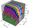
Figure 2: Fidelity versus $\tau\delta\omega_{jk}$ and $\tau D_{jk}$. The average wave function overlap between dynamics calculated exactly and dynamics calculated with zeroth order average Hamiltonian theory. This simulation averages over 3 random initial pure states, and uses $\phi_{j}=0.7$, $\omega^{j}_{\rm RF}=\delta\omega_{jk}/100.$

The fidelity between the spin states calculated by these two methods is calculated for different parameters $D_{jk}\tau$ and $(\delta\omega_{j}-\delta\omega_{k})\tau=\delta\omega_{jk}\tau.$ The simulation is run several times, averaging over random initial pure states. The resulting average fidelity is shown in Fig. 2. We find that if $\tau$ is short enough in comparison to $D_{jk}$ and $\delta\omega_{jk}$, the sequence works extremely well, and that errors due to a dipolar coupling which is too large or insufficient selectivity are independent, at least at the two-spin level.

III.3 Selective inversion for recoupling

The combination of a broadband decoupling pulse sequence and selective pulses allows independent single-qubit rotations, as discussed above. The coupling between a pair of nuclear spins also must be restored in order to perform two-qubit operations. We will demonstrate how to selectively recover the coupling between a pair of nuclear spins without affecting other nuclear spins.

We begin by applying rapid, broadband $\pi$-pulses that eliminate the offset term $H_{\rm Z}$. In what follows, these pulses are always applied on the fastest possible timescale. The average evolution under these $\pi$-pulses is therefore governed by the full dipolar term $\bar{H}_{\rm D}=H_{\rm D}$ [Eq. (3)]. We then manipulate this dipolar term with selective $\pi$-pulses. These selective pulses may be accomplished in the manner described in Sec. III.2, or by the usual soft NMR pulses if the dipolar coupling is sufficiently small. The broadband $\pi$-pulses must be suspended during these pulses to allow selectivity.

We now introduce a new “second-toggled” reference frame in which these selective rotations are treated as single, $\delta$-function rotations. “Free evolution” in the second-toggled frame corresponds to the average evolution during rapid broadband $\pi$ pulses only and the dipolar Hamiltonian, which is unaffected by those broadband $\pi$-pulses.

Working in this frame, we selectively rotate nucleus $k$ around the $x$-axis by $\pi$ ($X_{k}$). Then the second-toggled dipolar Hamiltonian is

$$H_{1}^{z}\equiv X_{k}H_{\rm D}^{z}X_{k}=D_{kl}(-2I_{k}^{z}I_{l}^{z}-I_{k}^{x}I_{l}^{x}+I_{k}^{y}I_{l}^{y}).$$ (25)

We further manipulate the second-toggled frame by applying broadband $\pi/2$ pulses that correspond to the usual WHH-4 sequences, except spacing them by a time $T$ chosen to be much longer than the selective pulse widths but much shorter than the dipolar dynamics. Thus, as in Sec. III.1, we have

$$\begin{array}[]{l}\tilde{\bar{H}}_{1}(\mbox{\hskip 4.30554pt}0^{+}<t<\mbox{\hskip 4.30554pt}T^{-})=H_{1}^{z},\\ \tilde{\bar{H}}_{1}(\mbox{\hskip 4.30554pt}T^{+}<t<2T^{-})=P_{\bar{x}}H_{1}^{z}P_{x},\\ \tilde{\bar{H}}_{1}(2T^{+}<t<4T^{-})=P_{\bar{x}}P_{y}H_{1}^{z}P_{\bar{y}}P_{x},\\ \tilde{\bar{H}}_{1}(4T^{+}<t<5T^{-})=P_{\bar{x}}H_{1}^{z}P_{x},\\ \tilde{\bar{H}}_{1}(5T^{+}<t<6T^{-})=H_{1}^{z},\end{array}$$ (26)

which averages to

$$\bar{\bar{H}}_{1} =\frac{1}{6T}\left(2TH^{z}_{1}+2TP_{\bar{x}}H^{z}_{1}P_{x}+2TP_{\bar{x}}P_{y}H^{z}_{1}P_{\bar{y}}P_{x}\right)$$

$$=-\frac{2}{3}D_{kl}^{\phantom{z}}(2I_{k}^{x}I_{l}^{x}+I_{k}^{y}I_{l}^{y}).$$ (27)

We refer to this sequence as the $W_{k}(X)$ sequence.

Three more subcycles are required. In the $W_{k}(Y)$ cycle, we selectively rotate nucleus ${k}$ around the $y$-axis by $\pi$ ($Y_{k}$). The dipole coupling in the second-toggled frame is then

$$H^{z}_{2}\equiv Y_{k}H_{\rm D}^{z}Y_{k}=D_{kl}^{\phantom{z}}(-2I_{k}^{z}I_{l}^{z}+I_{k}^{x}I_{l}^{x}-I_{k}^{y}I_{l}^{y}).$$ (28)

Again taking this evolution through a WHH-4 cycle with pulse-interval $T$, the second-averaged coupling averages to

$$\bar{\bar{H}}_{2} =\frac{1}{6T}\left(2TH^{z}_{2}+2TP_{\bar{x}}H^{z}_{2}P_{x}+2TP_{\bar{x}}P_{y}H^{z}_{2}P_{\bar{y}}P_{x}\right)$$

$$=-\frac{2}{3}D_{kl}^{\phantom{z}}(2I_{k}^{z}I_{l}^{z}+I_{k}^{y}I_{l}^{y}).$$ (29)

In the $W_{k}(Z)$ subcycle, we selectively rotate nucleus ${k}$ around the $z$-axis by $\pi$ ($Z_{k}$).

The double-toggled dipole coupling is

$$H^{z}_{3}\equiv D_{kl}^{\phantom{z}}(2I_{k}^{z}I_{l}^{z}+I_{k}^{x}I_{l}^{x}+I_{k}^{y}I_{l}^{y}),$$ (30)

which averages to

$$\bar{\bar{H_{3}}} =\frac{1}{6T}\left(2TH^{z}_{3}+2TP_{\bar{x}}H^{z}_{3}P_{x}+2TP_{\bar{x}}P_{y}H^{z}_{3}P_{\bar{y}}P_{x}\right)$$

$$=\frac{4}{3}D_{kl}^{\phantom{z}}(I_{k}^{x}I_{l}^{x}+I_{k}^{y}I_{l}^{y}+I_{k}^{z}I_{l}^{z})$$

$$=\frac{4}{3}D_{kl}^{\phantom{z}}{\bf I}_{k}\cdot{\bf I}_{l}$$ (31)

over a slow WHH-4 cycle. Finally, in the $W_{k}(-)$ subcycle, we do not apply any selective pulses to nucleus $k$. In this case, our subcycle is just a fast WHH-4 where a $W_{k}(X)$ cycle would have its selective $X_{k}$ pulse, combined with a slow WHH-4 cycle. The resulting second-averaged Hamiltonian is nothing more than the dipolar coupling $H_{\rm D}^{z}$ averaged through a WHH-4 cycle, which is of course zero.

In this way, three kinds of effective dipole coupling Hamiltonians for a pair of nuclear spins are generated by selective inversion of one or two of the nuclear spins under a slow WHH-4 sequence. The important observation is that the sum of these three effective Hamiltonians is zero:

$$\bar{\bar{H_{1}}}+\bar{\bar{H_{2}}}+\bar{\bar{H_{3}}}=0.$$ (32)

This fact will be used to decouple unwanted couplings when the coupling between a specific pair of nuclear spins is recovered.

Suppose we apply the $W_{k}(\alpha)$ subcycle to nucleus $k$ simultaneous with the $W_{k}(\beta)$ subcycle to nucleus $l$ ($\alpha$, $\beta$ = $-$, $X$, $Y$, $Z$). The resulting second-averaged effective coupling Hamiltonian between the two spins will be $\bar{\bar{H}}_{1}$, $\bar{\bar{H}}_{2}$, or $\bar{\bar{H}}_{3}$ if $\alpha\neq\beta$, or 0 if $\alpha=\beta$. Table 1 summarizes all of the possibilities.

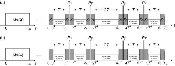
Figure 3: (a) Sequence $W_{k}(X)$: Within each time-interval of a slow broadband WHH-4 sequence (consisting of $\pi/2$-pulses $P_{x}$, $P_{\bar{x}}$, $P_{y}$ and $P_{\bar{y}}$), selective $\pi$-pulses around the $x$-axis (represented by $X_{k}$) are inserted at the beginning and at the end of the interval. Between the two selective $\pi$-pulses in an interval, fast broadband $\pi$-pulses are constantly applied at a speed faster than $1/\delta\omega$ in order to eliminate the Zeeman term. The selective $\pi$ pulses are produced by the combination of a broadband decoupling sequence and selective pulses. Sequences $W_{k}(Y)$ and $W_{k}(Z)$ are obtained by replacing $\pi$-pulses around the $x$-axis ($X_{k}$) by ones about the $y$-axis ($Y_{k}$) and the $z$-axis ($Z_{k}$), respectively. (b) Sequence $W(-)$: No selective $\pi$-pulses are applied. The fast broadband $\pi$-pulses and a broadband decoupling sequence are synchronized with the sequences $W_{k}(X)$, $W_{k}(Y)$ or $W_{k}(Z)$ that are applied to other spins.

Table 1: Effective Hamiltonian generated by selective $\pi$-pulses under a slow WHH-4 sequence. For example, when sequence $W(X)$ (See Fig. 3) is applied to $I_{k}$ and $W(-)$ to $I_{l}$, the effective Hamiltonian over the cycle is $\bar{\bar{H}}_{1}$, Eq. (27). When the same sequence is applied to both spins, the dipole coupling is the same as the natural dipole coupling Hamiltonian $H_{\rm D}^{z}$ [Eq. (3)] and averages to zero over a slow WHH-4 cycle.

	$W_{l}(-)$	$W_{l}(X)$	$W_{l}(Y)$	$W_{l}(Z)$
$W_{k}(-)$	0	$\bar{\bar{H}}_{1}$	$\bar{\bar{H}}_{2}$	$\bar{\bar{H}}_{3}$
$W_{k}(X)$	$\bar{\bar{H}}_{1}$	0	$\bar{\bar{H}}_{3}$	$\bar{\bar{H}}_{2}$
$W_{k}(Y)$	$\bar{\bar{H}}_{2}$	$\bar{\bar{H}}_{3}$	0	$\bar{\bar{H}}_{1}$
$W_{k}(Z)$	$\bar{\bar{H}}_{3}$	$\bar{\bar{H}}_{2}$	$\bar{\bar{H}}_{1}$	0

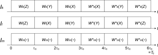
Figure 4: Super-WHH sequence to couple nuclear spins $I_{k}$ and $I_{l}$ while decoupling the rest of the spins in a system $I_{m}$ from both. In the sequence $W^{\ast}_{k}(\alpha)$, the phase and the order of the broadband $\pi$-pulses are rearranged such that $W^{\ast}_{k}(\alpha)$ has a time-reflection symmetry to $W_{k}({\alpha})$. Nuclear spins with the same frequency are decoupled by this sequence as well. The restored dipole coupling between $I_{k}$ and $I_{l}$ is $(8/9)A_{kl}{\bf I}_{k}.{\bf I}_{l}$.

Now we show how to recouple two spins $k$ and $l$ while the rest of the spins, represented by $m$ in the following, are decoupled from both spins $k$ and $l$. Couplings between ensemble nuclei (that is, nuclei with the same frequency) are also removed. Apply $W_{k}(Z)$, $W_{k}(Y)$ and $W_{k}(X)$ sequentially to $I_{k}$ while applying $W_{m}(-)$ three times to $I_{m}$, as shown in Fig. 4. The effective coupling over this supercycle, consisting of three slow WHH-4 cycles with cycle time $\tau_{\text{c}}=6T$, is averaged to

$$\frac{1}{3\tau_{\text{c}}}\left(\tau_{\text{c}}\bar{\bar{H}}_{3}+\tau_{\text{c}}\bar{\bar{H}}_{2}+\tau_{\text{c}}\bar{\bar{H}}_{1}\right)=0.$$ (33)

The dipole coupling among $m$ spins is decoupled as well.

To spin $I_{l}$, apply $W_{l}(Z)$, $W_{l}(X)$ and $W_{l}(Y)$ in this order. The dipole coupling between $I_{l}$ and $I_{m}$ is again averaged to zero. The coupling between $I_{k}$ and $I_{l}$ is, however,

$$\frac{1}{3\tau_{\text{c}}}\left(0+\tau_{\text{c}}\bar{\bar{H}}_{3}+\tau_{\text{c}}\bar{\bar{H}}_{3}\right)=\frac{8}{9}D_{kl}{\bf I}_{k}.{\bf I}_{l},$$ (34)

In this way, the two spins $k$ and $l$ are recoupled according to Eq. (34) while the rest of nuclear spins remain decoupled from spins $k$ and $l$ and from each other.

The present scheme works only in zeroth order in AHT. Dipolar terms of order $n$ scale as $\tau_{\text{c}}^{n}D_{kl}^{n+1}$ for other spins in the system with couplings as large as $D_{kl},$ including spins distant from $k$ and $l$ which are supposed to be decoupled. To compensate for this, we must make $\tau_{\text{c}}\ll D_{kl}^{-1}$ and perform quantum logic over many cycles. The resulting phase error for decoupled qubits over a logic gate lasting $t\sim D_{kl}^{-1}$ scales as $(\tau_{\text{c}}D_{kl})^{n}$. In the perfect-pulse limit, all odd order terms can be eliminating by simply symmetrizing the sequence, so that spin $k$ sees

$$W_{k}(Z)\ -\ W_{k}(Y)\ -\ W_{k}(X)\ -\ W^{\ast}_{k}(X)\ -\ W^{\ast}_{k}(Y)\ -\ W^{\ast}_{k}(Z).$$

and spin $l$ sees

$$W_{k}(Z)\ -\ W_{k}(X)\ -\ W_{k}(Y)\ -\ W^{\ast}_{k}(Y)\ -\ W^{\ast}_{k}(X)\ -\ W^{\ast}_{k}(Z).$$

In the sequence $W^{\ast}_{k}(\alpha)$, the phases and the orders of the selective pulses are re-arranged such that $W^{\ast}_{k}(\alpha)$ is time symmetrical to $W_{k}(\alpha)$. We refer to this sequence as “super-WHH.” Its cycle time is $T_{\text{c}}=6\tau_{\text{c}}=36T$.

IV Feasibility of the Proposed Scheme

Although the present scheme does not suffer from the $O(n)$ scaling of previous constructions,Leung et al. (2000) it can only work if the various timescales of the problem are well separated and high power pulses are available. In this section we discuss the feasibility of these assumptions.

The approximations we used are summarized in Table 2.

Table 2: Timescales. It is assumed in the present scheme that each timescale is much faster than the one below it. Expected orders of magnitude for these timescales are shown in the right column.

Rate	Description	rad/s
$\omega_{0}$	Average Larmor frequency	$10^{9}$
$\Omega_{\rm RF}$	Rabi frequency for broadband pulses	$10^{8}$
$n\delta\omega$	Number of qubits in gradient times gradient-induced frequency separation	$10^{5}n$
$\delta\omega$	Gradient-induced frequency separation	$10^{5}$
$\omega_{\rm RF}$	Rabi frequency for selective pulses	$10^{3}$
$T_{\text{c}}^{-1}$	Inverse of super-WHH cycle time	10
$D_{kl}$	Near-neighbor dipolar coupling constant	1
$D_{\rm iso}$	Intra-ensemble dipolar coupling constant	0.01

We now discuss the approximations made, the physical constraints behind them, the error created, and potential improvements.

IV.1 High DC field: $\omega_{0}\gg\Omega_{\rm RF}\gg n\delta\omega$

Laboratory magnetic fields rarely exceed 10-20 T due to the finite critical currents in existing superconductors. Obviously, it is beneficial to have as large an external field as is available for this scheme, as the Larmor frequency sets the ultimate physical timescale for the computation rate. If some qubits see an external field comparable to $\Omega_{\rm RF}$, then nonsecular terms become important and Bloch-Siegert shifts must be considered. Phase errors due to Bloch-Siegert shifts scale as $(\Omega_{\rm RF}/\omega_{0})^{2}$.

IV.2 High RF power: $\Omega_{\rm RF}\gg n\delta\omega\gg\delta\omega$

Although the present scheme does not slow down as qubits are added, maintaining the availability of broadband pulses becomes more difficult as the number of qubits gets large. However, the amount of RF power available is limited only by such issues as heat dissipation and arcing. With careful engineering and the use of microcoils,Webb (1997) Rabi frequencies approaching the Larmor frequency are attainable. Phase errors due to insufficiently broadband pulses scale for the most off-resonant nuclei as $(n\delta\omega/\Omega_{\rm RF})^{2}$.

Since $\Omega_{\rm RF}$ is ultimately limited by the Larmor frequency $\omega_{0}$, it would seem that the present scheme puts an upper limit on $n$, at least for reasonable clock speeds. Further, if the RF power remains constant and the dipole coupling is weakened as $n$ is increased, an $O(n)$ slowdown is again incurred. However, even if finite power is assumed, $n$ need not be the total number of qubits in the system. One could imagine instead a field gradient of finite extent, in which only a subset $n$ in a much larger set of qubits $N$ is well-distinguished by the field gradient, while all $N$ lie within a finite bandwidth accessible by the available RF power. The entire register can be accessed by moving the gradient, which could be done by switching of different gradient coils (as in magnetic resonance imaging), by mechanical motion of ferromagnets (as in magnetic resonance force microscopy), or by more exotic means involving manipulation of local electronic hyperfine fields. By limiting a moveable gradient to a small subsection of the qubit register in this way, sufficiently broadband pulses can be applied with finite power; the qubits poorly distinguished by weaker gradients are still decoupled by the present scheme. It is important to realize that such concerns will only be important in very large quantum computers with thousands of qubits.

IV.3 High field gradients or chemical shifts: $\delta\omega\gg\omega_{\rm RF}\gg T_{\text{c}}^{-1}$

Large gradients or chemical shifts are needed so that selective pulses do not become prohibitively long. Very large field gradients are attainable by a variety of means. Gradients as large as $\sim$10 T/$\mu$m with sufficient field homogeneity for sustaining measurable qubit ensembles can be made with ferromagnets.Goldman et al. (2000) The qubit-qubit frequency separation $\delta\omega$ can be made higher than $10$ kHz by suitably separating the qubits. Errors due to selective pulses affecting nearby nuclei scale as $\text{sinc}(\pi\delta\omega/2\omega_{\rm RF})$. Compensation schemes for such errors are possible.Steffen et al. (2000)

Although an ideal symmetric sequence has a vanishing first order term, a first order term does arrive in the presence of pulse errors and finite pulse width. For the simple sequences proposed here, the first order terms linear in the pulse width can only be neglected when the pulse widths of the selective pulses are much shorter than the cycle time. First order correction terms scale linearly with $1/\omega_{\rm RF}T_{\text{c}}$. It is important to note, however, that compensation for finite pulse widths in multiple pulse sequences can be achieved to high order by various means.Mehring (1983)

IV.4 Slow dipole couplings: $T_{\text{c}}^{-1}\gg D_{kl}\gg D_{\text{iso}}$

The timescale limitations discussed above limit the dipole coupling strengths which can be manipulated by this sequence. As discussed in Sec. III.3, $n^{\text{th}}$ order residual terms in the super-WHH sequence result in phase errors of order $(D_{kl}T_{\text{c}})^{n}$. Higher-order sequences can alleviate this restriction, but in the presence of non-idealities it is challenging to eliminate all second order terms. For the numbers used in Table 2, the dipole coupling must then be slower than 1 Hz, which is possible for reasonably separated nuclei, especially if $\gamma$ is low. Unfortunately, this results in rather slow clock times. Although coherence times can be extremely long,Ladd et al. (2004) the exponential speedup of quantum algorithms can only compensate for this large, constant slow-down over classical computers for very large problem sizes. Previous proposals for NMR computersLeung et al. (2000) are no faster, as the clock speed for such computers with several hundred qubits would also fall slower than a hertz. We re-emphasize the important advantage to the present scheme: there is no adverse scaling with $n$ with the super-WHH sequence. Therefore, if the clock cycle can be improved with higher magnetic fields, larger gradients, and error compensation schemes, the scheme will remain scalable for large quantum computers.

The final issue not resolved by the present scheme has been discussed elsewhere.Ladd et al. (2002) Copies of qubits in a single ensemble are decoupled by the compound WHH cycles of the present scheme. However, when different qubits $k$ and $l$ are coupled, all of the spins in ensemble $k$ are coupled to all of the spins in ensemble $l$, leading to cross-couplings which ultimately couple ensemble members. This may only be compensated for in the present scheme and in existing proposals by spatially separating ensemble members in order to ensure that qubit couplings are much stronger than couplings within each ensemble. This limits available couplings to near-neighbor couplings only.Ladd et al. (2002)

V Conclusion

We have seen that the judicious use of hard and selective pulses allows rotations of single-spin ensembles and selective couplings between ensembles. Single-spin rotations are performed by application of a weak RF field in conjunction with a rapid broadband decoupling sequence. Couplings between ensembles are accomplished by altering slower decoupling sequences with selective rotations, and constructing supercycles of such altered subsequences which couple only desired nuclei. The feasibility of this approach depends on the selection of a physical system that exhibits a hierarchy of time scales. These time scales must be widely separated to minimize the phase error of hard pulses, ensure the selectivity of soft pulses, minimize the impact of finite pulse widths, abate higher-order contributions to the average Hamiltonian, and mitigate inter-ensemble cross-couplings. In solid-state quantum computer architectures where these time-scale constraints are satisfied, the present scheme resolves two previously unresolved issues, improving the temporal scalability of such architectures: the linear slowdown of logic operations; and the complication of added intra-ensemble couplings.