Decoherence in a $N$-qubit solid-state quantum register

Abstract

We investigate the decoherence process for a quantum register composed of $N$ qubits coupled to an environment. We consider an environment composed of one common phonon bath and several electronic baths. This environment is relevant to the implementation of a charge based solid-state quantum computer. We explicitly compute the time evolution of all off-diagonal terms of the register’s reduced density matrix. We find that in realistic configurations, ”superdecoherence” and ”decoherence free subspaces” do not exist for an $N$-qubit system. This means that all off-diagonal terms decay, but not faster than $e^{-q(t)N}$, where $q(t)$ is of the same order as the decay function of a single qubit.

I Introduction

A typical quantum computer would consist of a large number ($N$) of two-level quantum systems, coined qubits, where the level splitting of each qubit and the interaction between pairs of qubits is adjustable. Quantum operations are then obtained by varying these parameters along a scheme defined by a quantum algorithm. The physical system composed by the $N$ two level systems is our quantum register. In the ideal case, when the quantum register is isolated, the time evolution of an arbitrary initial state $\varphi_{i}$ of the register is unitary. Such an ideal quantum computer could be used to solve some problems more efficiently than classical computers. An important example is Shor’s quantum algorithm to factor an integer with $n$ digits in a time growing polynomially with $n$ instead of exponentially when using a classical computer.Shor (1997)

However, any realistic quantum computer is coupled in some way to an external environment, which leads to decoherence and dissipation. The quantum register becomes entangled with the environment, so that its effective evolution is not unitary anymore. There can also be energy transfers between the register and the environmental bath, which lead to dissipation and decoherence. However, dissipation is not a requirement for decoherence to occur.Dubé and Stamp (2001)

The quantum decoherence process is elegantly expressed in the framework of the reduced density matrix of the quantum register. When no coupling to the environment is present, the reduced density matrix simply follows a Heisenberg-type evolution. As soon as the coupling to the environment is introduced, the off-diagonal terms of the reduced density matrix of the register decay with respect to time. This is often referred to as phase damping. In the simplest case of a single two level system connected to an environment, the off-diagonal elements of the reduced density matrix decay exponentially in time as $\sim e^{-q(t)}$, where $t$ is the time and the function $q(t)$ depends on the strength of the coupling to the environment. In the context of quantum information processing, such a decoherence event can be expressed as a quantum error. Following a pioneering work by Shor Shor (1995), it was shown that it is possible to encode each qubit using a minimum of five qubits (the five qubit code) in conjunction with quantum error correction algorithm in order to ”repair” a faulty qubit.Bennett et al. (1996) This would enable an accurate quantum computation as long as the error rate is small. The drawback of all quantum error correction schemes is that at least five times as many qubits are necessary for the same operation than in the ideal case.

In the case where there are $N$ two level systems the situation is potentially much worst since the decoherence of the register cannot be simply expressed as a superposition of single qubit decoherence. Indeed, Palma et al. argued that the decay of the most off-diagonal elements goes like $\sim e^{-q(t)N^{2}}$ (superdecoherence), when all qubits are imbedded in a single bath.Palma et al. (1996) Such a dependence would jeopardize the use of quantum error correction algorithms as soon as $q(t)N^{2}$ approaches 1, since the error rate would simply become too large. A potential rescue to this problem was proposed with the existence of decoherence free subspaces.Reina et al. (2002)

In this article we investigate the decoherence of $N$ qubits in the context of a realistic collection of solid state two level systems (our qubits) imbedded in a semiconducting environment. More specifically, we consider the case where the two-level system is a single electron in a double quantum dot patterned in a two dimensional electron gas confined in a GaAs/AlGaAs heterostructure. These qubits are coupled to a common phonon bath and to additional independent electronic baths, representing the metallic leads which allow the control and operation of the qubits. Experimentally, a decoherence time of about 1 ns was recently measured in a single double quantum dot.Hayashi et al. (2003) For this system, we find that the decoherence, i.e., the decay of the most off-diagonal elements of the $N$-qubit reduced density matrix, goes like $e^{-q(t)N}$, a much slower decoherence rate that previously thought, but that decoherence free subspaces do not exist.

To obtain these results, we consider a model based on a scaled version of the experimental double quantum dot as seen in Fig. 1. Tanamoto showed that such a system can perform all the operations necessary for a quantum computer. Tanamoto (2000) Many other groups have also used similar coupled quantum dots geometries as model system for a qubit.Krasheninnikov and Openov (1996); Brum and Hawrylak (1997); Bandyopadhyay et al. (1998); Zanardi and Rossi (1998); Openov and Bychkov (1998); Balandin and Wang (1999); Sanders et al. (1999); Openov (1999); Biolatti et al. (2000); Fedichkin et al. (2000) While we use this particular system for our model, our results are in fact more general and remain qualitatively similar for different physical realizations.

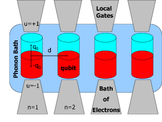
Figure 1: Schematic representation of a solid state quantum computer coupled to a common phonon bath and several independent electronic baths.

The rest of this article is organized as follows. In Section II we introduce the Hamiltonian, similar to a spin-boson model, and describe the $N$-qubit register, the environment and the coupling between the register and the environment. In Section III we give an exact formal expression for the reduced density matrix of the register. The time evolution of the reduced density matrix is expressed in terms of the influence functional, which is computed in Section IV. In these sections the expressions are fairly general and do not depend on the exact model considered. In order to gain insight into a physical system we consider the system shown in Fig. 1 in the next sections. Sections V and VI are devoted to the special case of acoustic phonons coupled to charge-qubits. The coupling to electronic baths is analyzed in section VII. In Section VIII we evaluate the decoherence rate for the coupling to a single phonon bath, where we show that the decoherence function scales as $e^{-q(t)N}$ when increasing the number, $N$ of qubits. We give physical estimates for piezo and deformation phonons in Section IX and analyze our results in the dynamical case in Section X, where we introduce quantum operations on the register and evaluate the decoherence process. Finally, a short summary and conclusions are given in the last section XI.

II The Hamiltonian

We use a Hamiltonian for our model qubit, which describes the tunneling of a single electron tunnelling between two adjacent quantum dots. The electronic state of the dots can be controlled by adjusting the gate voltage, which allows either localization of the electron or resonant tunnelling between the dots. The complete physical localization of the electron in a given dot is denoted by the vector $(1,0)^{\top}$ while localization in the other dot corresponds to $(0,1)^{\top}$. At low enough temperatures, only the combinations of these two states need to be taken into account. Each qubit is described by the Hilbert space $\mathbb{C}^{2}$ and the canonical basis is denoted by $|+1\rangle=(1,0)^{\top}$ and $|-1\rangle=(0,1)^{\top}$. The single qubit Hamiltonian reads (we write the Schrödinger equation as ${\rm i}\dot{\varphi}=H\varphi$, hence the units of $H$ are ${\rm s}^{-1}$)

$$H=-\Delta_{t}\sigma_{x}-\varepsilon_{t}\sigma_{z}\,,$$ (1)

where $\sigma_{x}$ and $\sigma_{z}$ denote the Pauli’s matrices, $\sigma_{z}|\pm 1\rangle=\pm|\pm 1\rangle$ and $\sigma_{x}|\pm 1\rangle=|\mp 1\rangle$. Typically, the tunnelling matrix element is $\Delta\sim 1-100GHz$ and the bias $\varepsilon$ is adjusted with the gate voltage. Both quantities need to be dynamically controlled for the operation of the qubit in a quantum computer.Tanamoto (2000)

For the $N$-qubit register, we write $|l\rangle$ (where $l\in\{-1,+1\}^{N}$) for the vector of $(\mathbb{C}^{2})^{\otimes N}$ defined as $|l\rangle:=|l_{1}\rangle\otimes\cdots\otimes|l_{N}\rangle$. The Hamiltonian of the register is decomposed as $H^{r}(t)=\Sigma(t)+\Delta(t)$, where $\Sigma(t)$ denotes the diagonal part of $H^{r}(t)$ with respect to the basis $|l\rangle$, that is $\Sigma(t)|l\rangle=\varepsilon(t,l)|l\rangle$.

For the total system, i.e., the register composed of $N$ qubits plus environment, we consider the following Hamiltonian

$$\begin{array}[]{ll}H(t)&\displaystyle=H^{r}(t)+H^{e}+H^{re}\\[5.69054pt] H^{e}&\displaystyle=\sum_{\bf{k}}\omega_{k}b_{\bf k}^{\dagger}b_{\bf k}\\[11.38109pt] H^{re}&=\displaystyle\sum_{\bf k}\phi_{\bf k}b_{\bf k}^{\dagger}+\phi_{\bf k}^{\dagger}b_{\bf k}\,,\end{array}$$ (2)

where $\phi_{\bf k}$ are operators acting on the register’s Hilbert space. We assume that they are diagonal with respect to the basis $|l\rangle$. The field operators $b_{\bf k}$ and $b_{\bf k}^{\dagger}$ are bosonic operators, that is

$$\left[b_{{\bf k}^{\prime}},b_{{\bf k}}^{\dagger}\right]=\delta_{{\bf k}^{\prime}{\bf k}}\,,$$ (3)

and all other commutators are zero. The Hamiltonian given in Eq. (2) is very general and is frequently used to study open quantum systems. It leads directly to the spin-boson model, which describes many types of environments with extended degrees of freedom (phonons, electrons, magnons…) and can be obtained from microscopic models. Leggett et al. (1987); Palma et al. (1996); Weiss (1999) It is however inappropriate for localized environments, such as a bath of nuclear spins. Prokof’ev and Stamp (2000)

We decompose $H(t)$ as $H(t)=H_{0}(t)+\Delta(t)$ with

$$H_{0}(t)=\Sigma(t)+H^{e}+H^{re}\,.$$ (4)

Note that $\langle l|H_{0}(t)|m\rangle=\delta_{lm}(\varepsilon(t,m)+H^{e}+H^{re}(m))$ where

$$\begin{array}[]{ll}\displaystyle H^{re}(m)&=\displaystyle\sum_{\bf k}\phi_{\bf k}(m)b_{\bf k}^{\dagger}+{\phi_{\bf k}(m)}^{*}b_{\bf k}\\[11.38109pt] \phi_{\bf k}(m)&\displaystyle=\langle m|\phi_{\bf k}|m\rangle\,.\end{array}$$ (5)

As a consequence, we find that the evolution operator associated to $H_{0}(s)$ is given by

$$\langle l|U_{0}(t,0)|m\rangle=\delta_{lm}\,{\rm e}^{-{\rm i}\int_{0}^{t}\varepsilon(s,m)ds}{\rm e}^{-{\rm i}t(H^{e}+H^{re}(m))}\,.$$ (6)

III Exact formal expression for the reduced density matrix

We now give an exact formal expression for the reduced density matrix of the register by expanding the evolution operator of the total system with respect to $\Delta(t)$, the off-diagonal terms of $H^{r}(t)$. This corresponds to the method of Leggett et al studied at length for the spin-boson model in Ref. Leggett et al. (1987).

The density matrix of the total system is given by $\rho(t)=U(t,0)\rho_{0}U(t,0)^{\dagger}$ where $\rho_{0}$ is the density matrix at time $t=0$ and $U(t,0)$ is the evolution operator associated to the total Hamiltonian $H(s)$. We define the interaction picture with respect to $H_{0}(s)$ as $\widetilde{\rho}(t)=U_{0}(t,0)^{\dagger}\rho(t)U_{0}(t,0)$. Hence, the Heisenberg equation reads ${\rm i}\dot{\widetilde{\rho}}(t)=L(t)\widetilde{\rho}(t)$, where $L(t)$ is the Liouville operator $L(t)A=[\widetilde{\Delta}(t),A]$. Therefore we have $\rho(t)=U_{0}(t,0)({\rm T}\{\exp[-{\rm i}\int_{0}^{t}L(s)ds]\}\rho_{0})U_{0}(t,0)^{\dagger}$.

The density matrix of the register is defined by tracing out all the environment degrees of freedom $\rho^{r}(t)=\mathrm{Tr}_{e}[\rho(t)]$. So, we need to compute the trace over the degrees of freedom of the environment of terms of the form

$$\langle l|U_{0}(t,0)\widetilde{\Delta}(t^{\uparrow}_{p-j})\cdots\widetilde{\Delta}(t^{\uparrow}_{1})\rho_{0}\widetilde{\Delta}(t^{\downarrow}_{1})\cdots\widetilde{\Delta}(t^{\downarrow}_{j})U_{0}(t,0)^{\dagger}|m\rangle,$$ (7)

with $t_{1}^{\uparrow}\leq t_{2}^{\uparrow}\cdots\leq t^{\uparrow}_{p-j}$ and $t_{1}^{\downarrow}\leq t_{2}^{\downarrow}\cdots\leq t^{\downarrow}_{j}$. This term reduces to a sum over the all pair of maps $(\zeta^{\downarrow},\zeta^{\uparrow})$ defined on $[0,t]$ with values in $\{-1,+1\}^{N}$, constant by step, and with $\zeta^{\uparrow}(t^{-})=l$ and $\zeta^{\downarrow}(t^{-})=m$. More precisely, $\zeta^{\uparrow}$ is constant on each interval $[t^{\uparrow}_{r},t^{\uparrow}_{r+1}[$ where $0\leq r\leq p-j$, with $t_{0}^{\uparrow}=0$ and $t^{\uparrow}_{p-j+1}=t$. Moreover, $\zeta^{\uparrow}(t_{p-j}^{\uparrow})=l$. On the other hand, $\zeta^{\downarrow}$ is constant on each interval $[t^{\downarrow}_{s},t^{\downarrow}_{s+1}[$ where $0\leq s\leq j$, with $t_{0}^{\downarrow}=0$ and $t^{\downarrow}_{j+1}=t$. Moreover, $\zeta^{\downarrow}(t_{j}^{\downarrow})=m$. We write $\zeta^{\uparrow}_{r}$ for $\zeta^{\uparrow}(t_{r}^{\uparrow})$, and $\zeta^{\downarrow}_{s}$ for $\zeta^{\downarrow}(t_{s}^{\downarrow})$. With these notations, the term above becomes

$$\begin{array}[]{l}\displaystyle\sum_{(\zeta^{\downarrow},\zeta^{\uparrow})}\prod_{r=1}^{p-j}\prod_{s=1}^{j}\langle\zeta^{\uparrow}_{r}|\Delta(t^{\uparrow}_{r})|\zeta^{\uparrow}_{r-1}\rangle\langle\zeta^{\downarrow}_{s-1}|\Delta(t^{\downarrow}_{s})|\zeta^{\downarrow}_{s}\rangle\\[17.07164pt] \hskip 28.45274pt\times\langle\zeta^{\uparrow}_{p-j}|U_{0}(t,t^{\uparrow}_{p-j})|\zeta^{\uparrow}_{p-j}\rangle\cdots\langle\zeta^{\uparrow}_{0}|U_{0}(t^{\uparrow}_{1},0)|\zeta^{\uparrow}_{0}\rangle\\[11.38109pt] \hskip 28.45274pt\times\langle\zeta^{\uparrow}_{0}|\rho_{0}|\zeta^{\downarrow}_{0}\rangle\langle\zeta^{\downarrow}_{0}|U_{0}(0,t^{\downarrow}_{1})|\zeta^{\downarrow}_{0}\rangle\cdots\langle\zeta^{\downarrow}_{j}|U_{0}(t^{\downarrow}_{j},t)|\zeta^{\downarrow}_{j}\rangle\ .\end{array}$$ (8)

We now assume the register and the environment to be decoupled at time $t=0$, hence $\rho_{0}=\rho_{0}^{r}\otimes\rho_{0}^{e}$. Moreover the environment is assumed to be initially at thermal equilibrium which means that $\rho_{0}^{e}={\rm e}^{-\beta H^{e}}Z_{e}^{-1}$, where $\beta=\hbar/K_{B}T$, hence $\beta T\simeq 7.64\cdot 10^{-12}$ sK.

Let $\gamma$ be the path in the complex plane defined as $\gamma(s)=s$ for $s\in[0,t]$, $\gamma(s)=2t-s$ for $s\in]t,2t]$, and $\gamma(s)=-{\rm i}(s-2t)$ for $s\in]2t,2t+\beta]$. Define $\zeta(s)$ as $\zeta(s)=\zeta^{\uparrow}(\gamma(s))$ for $s\in[0,t]$, and $\zeta(s)=\zeta^{\downarrow}(\gamma(s))$ for $s\in]t,2t]$, and $\zeta(s)=0$ for $s\in]2t,2t+\beta]$. For $\lambda\geq 0$, we define

$$U_{\lambda}(s)={\rm T}\left\{\exp\left[-{\rm i}\int_{0}^{s}\dot{\gamma}(s^{\prime})\left(H^{e}+\lambda H^{re}(\zeta(s^{\prime}))\right)ds^{\prime}\right]\right\}\,.$$ (9)

Moreover, we define the influence functional as

$$Z_{\lambda}[\zeta]={1\over Z_{e}}\mathrm{Tr}_{e}[U_{\lambda}(2t+\beta)]\,.$$ (10)

Finally, if $p$ and $j$ are integers with $0\leq j\leq p$, we denote by $\Theta_{pj}$ the set of all pairs $(\Omega_{1},\Omega_{2})$ of subsets of $\{1,\cdots,p\}$ such that $\Omega_{1}=\{p_{1},\cdots,p_{j}\}$ and $\Omega_{2}=\{q_{1},\cdots,q_{p-j}\}$ with $p_{1}\leq\cdots\leq p_{j}$, and $q_{1}\leq\cdots\leq q_{p-j}$, and such that $\Omega_{1}\cup\Omega_{2}=\{1,\cdots,p\}$ (hence $\Omega_{1}\cap\Omega_{2}$ is empty). Moreover, given $0\leq t_{1}\leq\cdots\leq t_{p}\leq t$ and a pair $(\Omega_{1},\Omega_{2})$ in $\Theta_{pj}$, we define the maps $(\zeta^{\downarrow},\zeta^{\uparrow})$ as above with $t_{1}^{\uparrow}=t_{q_{1}},\cdots,t_{p-j}^{\uparrow}=t_{q_{p-j}}$ and with $t_{1}^{\downarrow}=t_{p_{1}},\cdots,t_{j}^{\downarrow}=t_{p_{j}}$. We denote the set of all pairs of maps $(\zeta^{\downarrow},\zeta^{\uparrow})$ obtained in that way by $\Upsilon_{pj}$.

With these definitions, we find the following exact formal expression for the reduced density matrix of the register

$$\begin{array}[]{l}\displaystyle\langle l|\rho^{r}(t)|m\rangle=\sum_{p=0}^{\infty}(-{\rm i})^{p}\int_{0}^{t}dt_{p}\int_{0}^{t_{p}}dt_{p-1}\cdots\int_{0}^{t_{2}}dt_{1}\sum_{j=0}^{p}(-1)^{j}\sum_{(\zeta^{\downarrow},\zeta^{\uparrow})\in\Upsilon_{pj}}\\[17.07164pt] \hskip 42.67912pt\displaystyle\langle\zeta^{\uparrow}_{0}|\rho^{r}_{0}|\zeta^{\downarrow}_{0}\rangle\left(\prod_{r=1}^{p-j}\prod_{s=1}^{j}\langle\zeta^{\uparrow}_{r}|\Delta(t^{\uparrow}_{r})|\zeta^{\uparrow}_{r-1}\rangle\langle\zeta^{\downarrow}_{s-1}|\Delta(t^{\downarrow}_{s})|\zeta^{\downarrow}_{s}\rangle\right)\exp\left[-{\rm i}\int_{0}^{t}\left[\varepsilon(s,\zeta^{\uparrow}(s))-\varepsilon(s,\zeta^{\downarrow}(s))\right]ds\right]Z_{1}[\zeta]\,.\end{array}$$ (11)

Here the elements of the reduced density matrix are expressed in terms of the influence functional $Z_{1}[\zeta]$, which describes the effect of the bath on the time evolution. In the next section we evaluate this influence functional.

IV The influence functional

To compute the influence functional $Z_{1}[\zeta]$ we follow the method used for the spin-boson model in Ref. Chang and Chakravarty (1985). We define $g_{\lambda}(s)=\partial_{\lambda}U_{\lambda}(s)$ and denote by $H_{\lambda}(s)$ the integrand in Eq. (9). Then, inverting $\partial_{s}$ and $\partial_{\lambda}$, we obtain ${\rm i}\dot{g_{\lambda}}(s)=\partial_{\lambda}\left\{H_{\lambda}(s)U_{\lambda}(s)\right\}$, hence

$${\rm i}\dot{g_{\lambda}}(s)=H_{\lambda}(s)g_{\lambda}(s)+\dot{\gamma}(s)H^{re}(\zeta(s))U_{\lambda}(s)\,.$$ (12)

Therefore, since $g_{\lambda}(0)=0$, we have that

$$g_{\lambda}(s)=-{\rm i}U_{\lambda}(s)\int_{0}^{s}U_{\lambda}^{\dagger}(s^{\prime})\dot{\gamma}(s^{\prime})H^{re}(\zeta(s^{\prime}))U_{\lambda}(s^{\prime})ds^{\prime}\,.$$ (13)

As a consequence, defining

$$h_{\lambda}(s)={{\rm i}\over Z_{e}Z_{\lambda}[\zeta]}\mathrm{Tr}_{e}\left\{U_{\lambda}(2t+\beta)U_{\lambda}^{\dagger}(s)H^{re}(\zeta(s))U_{\lambda}(s)\right\},$$ (14)

we find that

$$\partial_{\lambda}Z_{\lambda}[\zeta]=-\left(\int_{0}^{2t}\dot{\gamma}(s)h_{\lambda}(s)ds\right)Z_{\lambda}[\zeta]\,,$$ (15)

hence

$$Z_{1}[\zeta]=\exp\left[-\int_{0}^{1}d\lambda\int_{0}^{2t}\dot{\gamma}(s)h_{\lambda}(s)ds\right]\,,$$ (16)

since by definition, $Z_{0}[\zeta]=1$.

From Eq. (5) we can decompose $h_{\lambda}$ as a sum by defining

$$f^{+}_{{\bf k}}(s)={{\rm i}\over Z_{e}Z_{\lambda}[\zeta]}\mathrm{Tr}_{e}\left\{U_{\lambda}(2t+\beta)U_{\lambda}^{\dagger}(s)b_{\bf k}^{\dagger}U_{\lambda}(s)\right\}\,,$$ (17)

and $f^{-}_{{\bf k}}(s)$ by the same formula but with the annihilation operator $b_{\bf k}$ instead of the creation operator $b_{\bf k}^{\dagger}$. Whence, we have

$$h_{\lambda}(s)=\sum_{\bf k}\phi_{\bf k}(\zeta(s))f_{\bf k}^{+}(s)+{\phi_{\bf k}(\zeta(s))}^{*}f_{\bf k}^{-}(s)\,.$$ (18)

Further, from the Heisenberg equation, defining $\widetilde{b_{\bf k}^{\dagger}}(s)$ as $U_{\lambda}^{\dagger}(s)b_{\bf k}^{\dagger}U_{\lambda}(s)$, we obtain that

$${\rm i}\partial_{s}\widetilde{b_{\bf k}^{\dagger}}(s)=\dot{\gamma}(s)U_{\lambda}^{\dagger}(s)[b_{\bf k}^{\dagger},H^{e}+\lambda H^{re}(\zeta(s))]U_{\lambda}(s)\,.$$ (19)

Therefore, from the commutation relations for bosonic operators, we obtain for $f_{\bf k}^{\pm}$ the following differential equation

$$\partial_{s}f_{\bf k}^{\pm}(s)=\pm\dot{\gamma}(s)\left({\rm i}\omega_{k}f_{\bf k}^{\pm}(s)-\lambda\phi_{\bf k\mp}(\zeta(s))\right)\,,$$ (20)

where $\phi_{{\bf k}+}(m)$ is given by Eq. (5) and $\phi_{{\bf k}-}(m)$ is the complex conjugate of $\phi_{{\bf k}+}(m)$.

The solution of Eq. (20) is obviously given by

$$\begin{array}[]{l}\displaystyle f_{\bf k}^{\pm}(s)={\rm e}^{\pm{\rm i}\omega_{k}\gamma(s)}\bigg{(}f_{\bf k}^{\pm}(0)+\\[11.38109pt] \hskip 71.13188pt\displaystyle\left.\mp\lambda\int_{0}^{s}{\rm e}^{\mp{\rm i}\omega_{k}\gamma(s^{\prime})}\dot{\gamma}(s^{\prime})\phi_{\bf k\mp}(\zeta(s^{\prime}))ds^{\prime}\right)\,.\end{array}$$ (21)

Now, because of the invariance of the trace under permutations, we have the boundary condition $f_{\bf k}^{\pm}(2t+\beta)=f_{\bf k}^{\pm}(0)$. Hence, from Eq. (21) we find that

$$\begin{array}[]{l}\displaystyle f_{\bf k}^{\pm}(0)={\lambda{\rm e}^{\pm\beta\omega_{k}/2}\over 2\sinh(\beta\omega_{k}/2)}\\[11.38109pt] \hskip 42.67912pt\displaystyle\times\int_{0}^{t}{\rm e}^{\mp{\rm i}\omega_{k}s}\left[\phi_{{\bf k}\mp}(\zeta^{\uparrow}(s))-\phi_{{\bf k}\mp}(\zeta^{\downarrow}(s))\right]ds\,.\end{array}$$ (22)

Defining

$$\begin{array}[]{l}\displaystyle\Delta_{\bf k}(s)=\phi_{\bf k}(\zeta^{\uparrow}(s))-\phi_{\bf k}(\zeta^{\downarrow}(s))\\[11.38109pt] \displaystyle\Sigma_{\bf k}(s)=\phi_{\bf k}(\zeta^{\uparrow}(s))+\phi_{\bf k}(\zeta^{\downarrow}(s))\,,\end{array}$$ (23)

where $\phi_{\bf k}$ is given by Eq. (5), we find that the influence functional is given by

$$Z^{b}_{1}[\zeta]={\rm e}^{-{\rm i}X^{b}}{\rm e}^{-\Lambda^{b}}\,,$$ (24)

with

$$\begin{array}[]{l}\displaystyle\Lambda^{b}=\sum_{\bf k}\coth(\beta\omega_{k}/2)\\ \displaystyle\hskip 28.45274pt\times{\rm Re}\left[\int_{0}^{t}ds\int_{0}^{s}ds^{\prime}{\rm e}^{-{\rm i}\omega_{k}(s-s^{\prime})}{\Delta_{\bf k}(s)}^{*}\Delta_{\bf k}(s^{\prime})\right]\,,\end{array}$$ (25)

and

$$X^{b}=\sum_{\bf k}{\rm Im}\left[\int_{0}^{t}ds\int_{0}^{s}ds^{\prime}{\rm e}^{-{\rm i}\omega_{k}(s-s^{\prime})}{\Delta_{\bf k}(s)}^{*}\Sigma_{\bf k}(s^{\prime})\right]\,.$$ (26)

Recall that $\zeta^{\uparrow}$ and $\zeta^{\downarrow}$ are constant on each interval $[t_{j-1},t_{j}[$ with $1\leq j\leq p+1$ ($t_{0}=0$ and $t_{p+1}=t$). We define

$$\begin{array}[]{l}\displaystyle\Delta_{\bf k}^{j}=\Delta_{\bf k}(t_{j-1})\\[11.38109pt] \displaystyle\Sigma_{\bf k}^{j}=\Sigma_{\bf k}(t_{j})\,,\end{array}$$ (27)

and

$$\begin{array}[]{ll}q_{k}(t-t_{0})&\displaystyle=\int_{t_{0}}^{t}ds\int_{t_{0}}^{s}ds^{\prime}{\rm e}^{-{\rm i}\omega_{k}(s-s^{\prime})}\\[11.38109pt] &\displaystyle={-{\rm i}\over\omega_{k}}(t-t_{0})+{1\over\omega_{k}^{2}}\left[1-{\rm e}^{-{\rm i}\omega_{k}(t-t_{0})}\right]\ .\end{array}$$ (28)

Note that

$$\int_{t_{j-1}}^{t_{j}}ds\int_{t_{m-1}}^{t_{m}}ds^{\prime}{\rm e}^{-{\rm i}\omega_{k}(s-s^{\prime})}=M_{k}^{jm}\,,$$ (29)

where

$$\begin{array}[]{l}\displaystyle M_{k}^{jm}=q_{k}(t_{j}-t_{m-1})+q_{k}(t_{j-1}-t_{m})\\[5.69054pt] \hskip 85.35826pt\displaystyle-q_{k}(t_{j}-t_{m})-q_{k}(t_{j-1}-t_{m-1})\,.\end{array}$$ (30)

Hence, we find that

$$\begin{array}[]{ll}\displaystyle\Lambda^{b}&\displaystyle=\sum_{\bf k}\coth(\beta\omega_{k}/2)\sum_{j=1}^{p+1}{\rm Re}\left[q_{k}(t_{j}-t_{j-1}){\Delta_{\bf k}^{j}}^{*}\Delta_{\bf k}^{j}\right]\\[17.07164pt] &\hskip 91.04872pt\displaystyle+\sum_{j=2}^{p+1}\sum_{m=1}^{j-1}{\rm Re}\left[{\Delta_{\bf k}^{j}}^{*}\Delta_{\bf k}^{m}M_{k}^{jm}\right]\,,\end{array}$$ (31)

and

$$\begin{array}[]{ll}\displaystyle X^{b}&\displaystyle=\sum_{\bf k}\sum_{j=1}^{p+1}{\rm Im}\left[q_{k}(t_{j}-t_{j-1}){\Delta_{\bf k}^{j}}^{*}\Sigma_{\bf k}^{j-1}\right]\\[17.07164pt] &\hskip 71.13188pt\displaystyle+\sum_{j=2}^{p+1}\sum_{m=1}^{j-1}{\rm Im}\left[{\Delta_{\bf k}^{j}}^{*}\Sigma_{\bf k}^{m-1}M_{k}^{jm}\right]\,.\end{array}$$ (32)

V Charge-qubits

In order to evaluate the influence functional further we need to specify the form of the coupling in the Hamiltonian (2). Therefore, we will focus on the example represented in Fig. 1. We consider $N$ equidistant qubits, with two electronic gates per qubit. We denote by ${\bf q_{n}}$ the center of the qubit $n$ ($1\leq n\leq N$, we put ${\bf q_{1}}={\bf 0}$). For qubit 1, ${\bf q_{{}_{0}}}$ is the center of the upper dot and ${\bf-q_{{}_{0}}}$ the center of the lower dot ($q_{{}_{0}}=|{\bf q_{{}_{0}}}|$). Moreover, we write ${\bf d}={\bf q_{2}}-{\bf q_{1}}$, and $d=|{\bf d}|$, the distance between qubits. Hence ${\bf q_{n}}=(n-1){\bf d}$, and ${\bf q_{{}_{0}}}\cdot{\bf d}=0$. Each qubit has a single electron.

For $H^{re}$ we first consider the coupling between electrons in the qubits and longitudinal phonons. This can be described by a Fröhlich-type Hamiltonian Fröhlich (1954), where we have

$$\phi_{\bf k}=g(k)\sum_{n=1}^{N}{\rm e}^{-{\rm i}{\bf k}\left[(n-1){\bf d}+{\bf q_{{}_{0}}}\sigma_{z}^{n}\right]}\,,$$ (33)

where $\sigma_{z}^{n}$ is defined as $\sigma_{z}^{n}|l\rangle=l_{n}|l\rangle$. This form describes the coupling $g(k)$ between the charge of qubit $n$ localized at $(n-1){\bf d}+{\bf q_{{}_{0}}}\sigma_{z}^{n}$ and the phonon bath. Here, the spatial configuration is explicitly considered.

Since the optical phonons are gapped at low frequency they do not contribute to low temperature decoherence, only acoustic phonons are relevant. We also consider only a linear coupling between the phonons and the qubits. Nonlinear couplings can also be included and it has been shown that these can be mapped to an effective spin-boson model, albeit with decoherence rates (friction coefficients) that are very strongly temperature dependent Dubé and Stamp (1998a). Surface phonons are not considered either, since the quantum dots are usually embedded well inside the semiconductor. Moreover, we assume that the phonons are only coupled to the diagonal operators of the qubit and we do not consider any non-diagonal couplings (involving terms like $\sigma_{x}$ or $\sigma_{y}$) between the environment and the qubit. Such terms appear, e.g., when spin degrees of freedom become relevant Dubé and Stamp (2001); Prokof’ev and Stamp (2000). For charge qubits, nuclear spins are irrelevant and we restrict our study to the diagonal spin-boson model. In Sections VI, VII, and IX, we will further discuss the acoustic, electronic and deformation environmental degrees of freedom.

Introducing the notations

$$\begin{array}[]{ll}\xi(s)&\displaystyle={\left[\zeta^{\uparrow}(s)-\zeta^{\downarrow}(s)\right]\over 2}\\[5.69054pt] \chi(s)&\displaystyle={\left[\zeta^{\uparrow}(s)+\zeta^{\downarrow}(s)\right]\over 2}\,,\end{array}$$ (34)

we obtain that

$$\Delta_{\bf k}(s)=-2{\rm i}g(k)\sin({\bf kq_{0}})\sum_{n=1}^{N}{\rm e}^{-{\rm i}{\bf k}{\bf d}(n-1)}\xi_{n}(s)$$ (35)

and

$$\begin{array}[]{l}\displaystyle\Sigma_{\bf k}(s)=2g(k)\sum_{n=1}^{N}{\rm e}^{-{\rm i}{\bf k}{\bf d}(n-1)}\left\{\cos({\bf kq_{0}})\right.\\ \hskip 142.26378pt\left.\displaystyle-{\rm i}\chi_{n}(s)\sin({\bf kq_{0}})\right\}\,.\end{array}$$ (36)

Now, as before, we denote $\xi(t_{j-1})$ as $\xi^{j}$ and $\chi(t_{m})$ as $\chi^{m}$. Moreover, we denote by $J$ the $N\times N$ Jordan bloc $J_{ij}=\delta_{ji+1}$ and write $\upsilon=(1,{\rm e}^{{\rm i}{\bf kd}},\cdots,{\rm e}^{{\rm i}{\bf kd}(N-1)})$. With these notations, we find that

$$\begin{array}[]{ll}{\Delta_{\bf k}^{j}}^{*}\Delta_{\bf k}^{m}&\displaystyle=4|g(k)|^{2}\sin({\bf kq_{0}})^{2}\left(\langle\xi^{j}|\xi^{m}\rangle+\sum_{r=1}^{N-1}\langle\xi^{j}|J^{r}|\xi^{m}\rangle{\rm e}^{-{\rm i}{\bf k}{\bf d}r}+\langle\xi^{m}|J^{r}|\xi^{j}\rangle{\rm e}^{{\rm i}{\bf k}{\bf d}r}\right)\,,\end{array}$$ (37)

and

$$\begin{array}[]{ll}{\Delta_{\bf k}^{j}}^{*}\Sigma_{\bf k}^{m-1}&\displaystyle=4|g(k)|^{2}\sin({\bf kq_{0}})^{2}\left(\langle\xi^{j}|\chi^{m-1}\rangle+\sum_{r=1}^{N-1}\langle\xi^{j}|J^{r}|\chi^{m-1}\rangle{\rm e}^{-{\rm i}{\bf k}{\bf d}r}+\langle\chi^{m-1}|J^{r}|\xi^{j}\rangle{\rm e}^{{\rm i}{\bf k}{\bf d}r}\right)\\[17.07164pt] &\displaystyle\hskip 199.16928pt+{2|g(k)|^{2}\sin({\bf kq_{0}})\cos({\bf kq_{0}})\over\sin({\bf kd}/2)}{\rm e}^{{\rm i}{\bf kd}/2}\bigg{(}1-{\rm e}^{-{\rm i}{\bf kd}N}\bigg{)}\langle\xi^{j}|\upsilon\rangle\,.\end{array}$$ (38)

Hence, introducing the following notations for $r$ between $0$ and $N-1$ and $n$ between $1$ and $N$

$$\begin{array}[]{ll}Q^{r}_{2\pm}(t)&\displaystyle=2\sum_{\bf k}|g(k)|^{2}{1\over\omega_{k}^{2}}\coth(\beta\omega_{k}/2)\sin({\bf kq_{0}})^{2}\left[\cos({\bf k}{\bf d}r)-\cos(\omega_{k}t\pm{\bf k}{\bf d}r)\mp\omega_{k}t\sin({\bf k}{\bf d}r)\right],\\[17.07164pt] Q_{1\pm}^{r}(t)&\displaystyle=2\sum_{\bf k}|g(k)|^{2}{1\over\omega_{k}^{2}}\sin({\bf kq_{0}})^{2}\left[\sin(\omega_{k}t\pm{\bf kd}r)-\omega_{k}t\cos({\bf k}{\bf d}r)\mp\sin({\bf k}{\bf d}r)\right],\\[17.07164pt] \Psi_{n}(t)&\displaystyle=2\sum_{\bf k}|g(k)|^{2}{1\over\omega_{k}^{2}}\left[\sin(\omega_{k}t-{\bf kd}(n-1/2))-\sin(\omega_{k}t-{\bf kd}(n-1/2-N))\right]{\sin({\bf kq_{0}})\cos({\bf kq_{0}})\over\sin({\bf kd}/2)},\\[11.38109pt] \Phi_{n}&\displaystyle=2\sum_{\bf k}|g(k)|^{2}{1\over\omega_{k}}\left[\cos({\bf kd}(n-1/2))-\cos({\bf kd}(n-1/2-N))\right]{\sin({\bf kq_{0}})\cos({\bf kq_{0}})\over\sin({\bf kd}/2)}\,,\end{array}$$ (39)

we find that

$$\begin{array}[]{l}\displaystyle\sum_{\bf k}\coth(\beta\omega_{k}/2){\rm Re}\left[{\Delta_{\bf k}^{j}}^{*}\Delta_{\bf k}^{m}q_{k}(t)\right]=\sum_{r=0}^{N-1}\nu_{r}\left[\langle\xi^{j}|J^{r}|\xi^{m}\rangle Q_{2+}^{r}(t)+\langle\xi^{m}|J^{r}|\xi^{j}\rangle Q_{2-}^{r}(t)\right]\\[17.07164pt] \displaystyle\sum_{\bf k}{\rm Im}\left[{\Delta_{\bf k}^{j}}^{*}\Sigma_{\bf k}^{m-1}q_{k}(t)\right]=\sum_{r=0}^{N-1}\nu_{r}\left[\langle\xi^{j}|J^{r}|\chi^{m-1}\rangle Q_{1+}^{r}(t)+\langle\chi^{m-1}|J^{r}|\xi^{j}\rangle Q_{1-}^{r}(t)\right]+\sum_{n=1}^{N}\xi_{n}^{j}\left[\Psi_{n}(t)-\Psi_{n}(0)-\Phi_{n}t\right]\,,\end{array}$$ (40)

where $\nu_{r}$ is defined as $\nu_{0}=1$ and $\nu_{r}=2$ for $r\geq 1$. In the next section, we show that in the continuum limit, $\Psi_{n}(t)$ and $\Phi_{n}$ are zero and we provide compact formulas for $Q^{r}_{2\pm}(t)$ and $Q_{1\pm}^{r}(t)$. Note that from Eq. (40), the terms $X^{b}$ and $\Lambda^{b}$ of the influence functional (Eqs. (31) and (32)) can be expressed through the functions $Q_{1\pm}^{r}(t)$, $Q_{2\pm}^{r}(t)$, $\Psi_{n}(t)$ and $\Phi_{n}$.

VI Linear dispersion (acoustic phonons)

In order to simplify the expressions for $Q^{r}_{2\pm}(t)$ and $Q_{1\pm}^{r}(t)$ we need to specify the dispersion relation. Since we are interested in the effects of a phonon bath, the only relevant phonons at low temperatures are acoustic phonons, hence we assume a linear dispersion form $\omega_{k}\simeq c_{L}|{\bf k}|$, where $c_{L}$ is the speed of sound in the sample. We consider a cubic sample of volume $V_{S}=L_{1}L_{2}L_{3}$. The sum in $H^{e}$ and $H^{re}$ runs over all ${\bf k}=2\pi(n_{1}/L_{1},n_{2}/L_{2},$ $n_{3}/L_{3})$ with $n_{i}$ integers and $|{\bf k}|<a^{-1}$, where $a$ is the lattice constant which of the order of a few angströms. In the limit of an infinite volume, the sum over ${\bf k}$ can be replaced by and integral

$$\sum_{\bf k}\rightarrow{{V_{S}}\over(2\pi c_{L})^{3}}\int_{0}^{c_{L}a^{-1}}d\omega\omega^{2}\int_{0}^{\pi}d\theta\sin(\theta)\int_{0}^{2\pi}d\phi\,.$$ (41)

Further, we can assume that $g(\omega/c_{L})$ decreases in such a way that in (41) we can replace the bound $c_{L}a^{-1}$ by $+\infty$.

Recall that ${\bf q_{0}}$ and ${\bf d}$ are orthogonal. We choose

$$\begin{array}[]{ll}{\bf kq_{0}}&\displaystyle={\omega\over c_{L}}q_{0}\cos(\theta)\\[11.38109pt] {\bf kd}&\displaystyle={\omega\over c_{L}}d\sin(\theta)\cos(\phi)\,.\end{array}$$ (42)

Since

$$\begin{array}[]{l}\displaystyle\int_{0}^{\pi}\sin(y\cos(\theta))\cos(y\cos(\theta))g(\sin(\theta))\sin(\theta)d\theta\\[5.69054pt] \hskip 56.9055pt\displaystyle=\int_{-1}^{1}\sin(y\tau)\cos(y\tau)g(\sqrt{1-\tau^{2}})d\tau=0\,,\end{array}$$ (43)

for any function $g$ such that the integral exists, $\Phi_{n}$ and $\Psi_{n}(t)$ are equal to zero.

We now compute the functions $Q_{2\pm}^{r}$ and $Q_{1\pm}^{r}$. We first expand the expressions in $\cos(\omega_{k}t\pm{\bf kd}r)$ and $\sin(\omega_{k}t\pm{\bf kd}r)$ in terms of $\cos(\omega_{k}t)\cos({\bf kd}r)$ and $\sin(\omega_{k}t)\sin({\bf kd}r)$. Further, because $\int_{0}^{2\pi}f(\cos(\phi))d\phi=0$ for any odd function $f$, the terms in $\sin({\bf kd}r)$ do not contribute to the integral. Therefore, we can omit the indices $\pm$. We then introduce the transit time ($\tau_{s}$) and a dimensionless parameter $\alpha$

$$\tau_{s}={d\over c_{L}}\hskip 14.22636pt\text{and}\hskip 14.22636pt\alpha={2q_{0}\over d}\,.$$ (44)

The parameter $\alpha$ represents the ratio of the size of a qubit over the distance between qubits (typically, $\alpha$ is smaller than unity). Integrating over $\phi$ the term in $\cos({\bf kd}r)$ leads to a term $2\pi J_{0}^{B}(\omega\tau_{s}r\sin(\theta))$, where $J_{0}^{B}$ denotes the Bessel function of the first kind. To perform the integral over $\theta$, we use the formula ($z>0$)

$$\begin{array}[]{l}\displaystyle\int_{0}^{\pi}\sin^{2}(y\cos(\theta))J_{0}^{B}(z\sin(\theta))\sin(\theta)d\theta\\[5.69054pt] \hskip 85.35826pt\displaystyle={\sin(z)\over z}-{\sin\left(\sqrt{z^{2}+4y^{2}}\right)\over\sqrt{z^{2}+4y^{2}}}\,,\end{array}$$ (45)

to find

$$\begin{array}[]{l}\displaystyle Q_{2}^{r}(t)=\int_{0}^{\infty}{J_{r}(\omega)\over\omega^{2}}\left[1-\cos(\omega t)\right]\coth(\beta\omega/2)d\omega\\[11.38109pt] \displaystyle Q_{1}^{r}(t)=\int_{0}^{\infty}{J_{r}(\omega)\over\omega^{2}}\left[\sin(\omega t)-\omega t\right]d\omega\,,\end{array}$$ (46)

where the spectral function is given by

$$\begin{array}[]{l}\displaystyle J_{r}(\omega)=c_{1}\omega^{2}|g(\omega/c_{L})|^{2}\\[11.38109pt] \hskip 28.45274pt\displaystyle\times\left[\frac{\sin(\omega r/\alpha\omega_{q})}{\omega r/\alpha\omega_{q}}-\frac{\sin(\omega\sqrt{r^{2}+\alpha^{2}}/\alpha\omega_{q})}{\omega\sqrt{r^{2}+\alpha^{2}}/\alpha\omega_{q}}\right],\end{array}$$ (47)

with $c_{1}=V_{S}/(2\pi^{2}c_{L}^{3})$ and $\omega_{q}=(\alpha\tau_{s})^{-1}=c_{L}/2q_{0}$. The spectral function $J_{0}(\omega)$ is defined by taking the limit $r\rightarrow 0$ or

$$J_{0}(\omega)=c_{1}\omega^{2}|g(\omega/c_{L})|^{2}\left[1-\frac{\sin(\omega/\omega_{q})}{\omega/\omega_{q}}\right].$$ (48)

Our expression for $J_{0}$ has the same form as the one obtained for a single double quantum dot Brandes and Kramer (1999); Fedichkin and Fedorov (2004). Moreover, apart from the term linear in $t$ of $Q_{1}^{r}(t)$ and the $r$ dependence, Eq. (46) is identical to Eqs. (4.22a) and (4.22b) in Ref. Leggett et al. (1987). More importantly, the particular $r$-dependence of the spectral function in Eq. (47) is the main reason why the decoherence induced by the bath of phonons does not lead to “superdecoherence”. Indeed, if we expand $J_{r}$ in terms of $\alpha/r$ we obtain

$$J_{r}(\omega)\simeq-{c_{1}\over 2}\left({\alpha\omega\over r}\right)^{2}|g(\omega/c_{L})|^{2}\cos(r\omega/\alpha\omega_{q})\,,$$ (49)

when $\alpha\omega/(4r\omega_{q})\ll 1$. This $\sim 1/r^{2}$ dependence is responsible for the suppression of “superdecoherence”. In the unphysical limit, where $\alpha$, the ratio of the size of the qubit and the distance between qubits, is much greater than one, there is no dependence on $r$ for the expressions of $Q_{1}^{r}$ and $Q_{2}^{r}$ and the spectral function $J_{r}(\omega)$ equals $J_{0}(\omega)$, which leads to “superdecoherence”. It is interesting to note that our result for the influence functional differs from that of references Palma et al. (1996); Reina et al. (2002) because they have neglected the angle between ${\bf k}$ and ${\bf d}$ by introducing the “transit time” as $\omega t_{s}={\bf k}\cdot{\bf d}$.

The influence functional can now be written in a compact form by first defining

$$Q^{b}_{m}(t)=\sum_{r=0}^{N-1}\nu_{r}\left(J^{r}+{J^{\dagger}}^{r}\right)Q_{m}^{r}(t)\,,$$ (50)

with $m=1,2$. Hence, $2Q_{m}^{0}(t)$ are the diagonal elements of the $N\times N$ matrix $Q^{b}_{m}(t)$, and $2Q_{m}^{r}(t)$, with $r\neq 0$, the off-diagonal terms. Following a similar notation as in Ref. Leggett et al. (1987), we define

$$\begin{array}[]{l}\Lambda^{b}_{jk}=Q^{b}_{2}(t_{j}-t_{k-1})+Q^{b}_{2}(t_{j-1}-t_{k})\\[5.69054pt] \hskip 71.13188pt-Q^{b}_{2}(t_{j}-t_{k})-Q^{b}_{2}(t_{j-1}-t_{k-1})\,,\end{array}$$ (51)

and $X^{b}_{jk}$ by the same formula, but with $Q^{b}_{1}$ instead of $Q^{b}_{2}$. Note that the part linear in $t$ of $Q_{1}^{b}(t)$ does not contribute to $X^{b}_{jk}$. With these definitions, we find that

$$\begin{array}[]{l}\displaystyle\Lambda^{b}=\sum_{j=1}^{p+1}\langle\xi^{j}|Q^{b}_{2}(t_{j}-t_{j-1})|\xi^{j}\rangle+\sum_{j=2}^{p+1}\sum_{k=1}^{j-1}\langle\xi^{j}|\Lambda^{b}_{jk}|\xi^{k}\rangle\\[17.07164pt] \displaystyle X^{b}=\sum_{j=1}^{p+1}\langle\xi^{j}|Q^{b}_{1}(t_{j}-t_{j-1})|\chi^{{}_{j-1}}\rangle+\sum_{j=2}^{p+1}\sum_{k=1}^{j-1}\langle\xi^{j}|X^{b}_{jk}|\chi^{{}_{k-1}}\rangle,\end{array}$$ (52)

and the influence functional is then simply given by Eq. (24), where $\Lambda^{b}$ represents the exponential decay due to the coupling to the bath and $X^{b}$ describes the phase.

It is important to observe that for a single qubit (i.e. $N=1$) we recover the usual formula for the influence functional of the spin-boson model with the spectral function $J_{0}(\omega)$. Expressions (52) are evaluated quantitatively in Sections VIII and IX.

VII The coupling to other electrons

The coupling due to the metallic gates can either be provided by the two dimensional electron gas (lateral gates) or by metallic top gates. Each gate is considered as a gas of free electrons. The gates are labelled by $(n,u)$ with $u=+1$ for the gate above the qubit $n$, and $u=-1$ for the gate below the qubit $n$ (see Figure 1). The electron gas in the gate $(n,u)$ is described as

$$H^{f}_{nu}=\sum_{\bf{k}\,\sigma}E_{k}{f_{{\bf k}\sigma}^{nu}}^{\dagger}f_{{\bf k}\sigma}^{nu}\,,$$ (53)

where $f_{{\bf k}\sigma}^{nu}$ and ${f_{{\bf k}\sigma}^{nu}}^{\dagger}$ are fermionic operators. The gates are supposed to be isolated from each other, hence fermionic operators with different indices $n$ or different indices $u$ commute. We describe the coupling between the register and the electrons in the gates $(n,u)$ as

$$H^{rf}_{nu}=U_{nu}\sum_{{\bf k}{\bf k^{\prime}}\sigma}{f_{{\bf k}\sigma}^{nu}}^{\dagger}f_{{\bf k^{\prime}}\sigma}^{nu}$$ (54)

where $U_{nu}$ is an operator acting on the register’s Hilbert space

$$U_{nu}=u\sum_{j=1}^{N}V(|j-n|)\sigma_{z}^{j}\,.$$ (55)

If we add the sum over $n$ ranging from $1$ to $N$ and $u=\pm 1$ of $H^{f}_{nu}+H^{rf}_{nu}$ to the Hamiltonian (2), and compute again the reduced density matrix of the register, this leads to Eq. (11), where the bosonic influence functional is now multiplied by a fermionic influence functional $Z^{f}[\zeta]$ which is a product of fermionic influence functionals corresponding to each gate

$$Z^{f}[\zeta]=\prod_{n=1}^{N}\prod_{u=\pm 1}Z^{nu}[\zeta]\,.$$ (56)

The electron-electron coupling is given by the Coulomb potential. Since each gate is much closer to the corresponding qubit than the distance between qubits, we assume that $V(r)=0$ for $r\geq 1$ in Eq. (55). Hence, writing $V_{0}$ for $V(0)$, the interaction term reduces to $U_{nu}=uV_{0}\sigma_{z}^{n}$, and we are left with a two-level system coupled to a fermionic bath by a contact potential. This model has been studied in Ref. Chang and Chakravarty (1985), where it was shown that for a density of states $\rho(\epsilon)$ constant throughout the conduction band $E_{F}$ of the bath, i.e. $\rho(\epsilon)\simeq\rho_{0}{\rm e}^{-\epsilon/E_{F}}$ (hence $\rho_{0}=1/E_{F}$), the fermionic bath behaves as a bosonic environment with a spectral density of the ohmic form. This means, that aside from an adiabatic shift, i.e. a shift of the bias energy of the system, the influence functional $Z^{nu}[\zeta]$ is identical to the influence functional of the bosonic bath, provided $\phi_{\bf k}=g_{k}\sigma_{z}^{n}$ with $g_{k}$ real, and $\sum_{\bf k}g_{k}^{2}\delta(\omega-\omega_{k})=J(\omega)$, with a spectral density function of the ohmic form

$$J(\omega)=\eta\omega{\rm e}^{-\omega/\omega_{c}^{f}}\,,$$ (57)

where

$$\eta={2\over\pi^{2}}\arctan^{2}(\pi\rho_{0}V_{0})\,.$$ (58)

Here we use $\omega_{c}^{f}\simeq E_{F}/h$, where $E_{F}$ is the Fermi energy of the bath.

As a consequence, the influence functional becomes, $Z^{f}[\zeta]={\rm e}^{-{\rm i}X^{f}}{\rm e}^{-\Lambda^{f}}$, using Eqs. (23), (31) and (32), where $X^{f}$ and $\Lambda^{f}$ are given by Eq. (52) with the matrices $Q_{{}_{1,2}}^{f}(t)=8\;\mathsf{id}\;q_{{}_{1,2}}^{f}(t)$, where $\mathsf{id}$ denotes the identity $N\times N$ matrix, and $q_{{}_{1,2}}^{f}(t)$ is defined as in Eq. (46) with the spectral function given in Eq. (57). The factor $8$ comes on one hand from the sum over $u=\pm 1$, and on the other hand from the factor ${1\over 2}$ in Eq. (34).

VIII Decoherence function

We now compute the decreasing rate of the off-diagonal terms of the register’s reduced density matrix $\rho^{r}(t)$. As in Refs. Palma et al. (1996) and Reina et al. (2002), we consider the case where the dynamics of the register is trivial, i.e. $\Delta(t)\equiv 0$. This means that no quantum operation is performed. In this case, $\langle l|\rho^{r}(t)|m\rangle$ is simply given by the term $p=0$ in Eq. (11) and can be computed exactly. Note that the extension to N qubits in operation ($\Delta\neq 0$) is far from trivial Dubé and Stamp (1998b), and is discussed in Section X. If $\Delta(t)\equiv 0$, we find that

$$\begin{array}[]{l}\displaystyle\langle l|\rho^{r}(t)|m\rangle=\langle l|\rho_{0}^{r}|m\rangle\exp\left[-{\rm i}\int_{0}^{t}\left[\varepsilon(s,l)-\varepsilon(s,m)\right]ds\right]\\[17.07164pt] \hskip 142.26378pt\displaystyle\times Z_{1}^{b}[l,m]Z^{f}[l,m]\,.\end{array}$$ (59)

Moreover, we have

$$\begin{array}[]{ll}\Lambda^{b}&\displaystyle={1\over 4}\langle l-m|Q^{b}_{2}(t)|l-m\rangle\\[5.69054pt] X^{b}&\displaystyle={1\over 4}\langle l-m)|Q^{b}_{1}(t)|l+m\rangle\\[5.69054pt] \Lambda^{f}&\displaystyle=2\|l-m\|^{2}q_{2}^{f}(t)\\[5.69054pt] X^{f}&\displaystyle=0\,.\end{array}$$ (60)

For the diagonal terms (i.e. $l=m$), $\Lambda^{b}=0$ and $\Lambda^{f}=0$, whereas for the off-diagonal terms, with Eq. (50) we have

$$\begin{array}[]{l}\displaystyle\Lambda^{b}={1\over 2}Q_{2}^{0}(t)\|l-m\|^{2}\\[11.38109pt] \hskip 28.45274pt\displaystyle\times\left[1+2\sum_{r=1}^{N-1}{\langle l-m|J^{r}|l-m\rangle\over\|l-m\|^{2}}{Q_{2}^{r}(t)\over Q_{2}^{0}(t)}\right]\,.\end{array}$$ (61)

Therefore, for the most off-diagonal terms (i.e. $l-m=2(1,\cdots,1)$), we find

$$\begin{array}[]{ll}\Lambda^{b}&\displaystyle=2NQ_{2}^{0}(t)\left(1+e(t,N)\right)\\[5.69054pt] X^{b}&=0\\[5.69054pt] \Lambda^{f}&\displaystyle=8Nq_{2}^{f}(t)\,,\end{array}$$ (62)

with

$$e(t,N)=2\sum_{r=1}^{N-1}\left(1-{r\over N}\right){Q_{2}^{r}(t)\over Q_{2}^{0}(t)}\,,$$ (63)

which is small and bounded in the variable $N$ since $Q_{2}^{r}\simeq r^{-2}$ as discussed in section VI. This implies that the decreasing rate is proportional to the number $N$ of qubits in the register. Note that if we neglect the $r$ dependence and put $Q^{r}_{2}(t)=q_{2}(t)$, for all $r\geq 1$, we find the result stated in Refs. Palma et al. (1996); Reina et al. (2002).

The decoherence functions evaluated above are the ones corresponding to the most off-diagonal elements of the density matrix. They correspond to the maximum decoherence rate of the register. For other matrix elements, the bound $|\langle\xi|J^{n}|\xi\rangle|\leq\|\xi\|^{2}$ leads to

$$b_{-}(t)\leq|\langle l|\rho^{r}(t)|m\rangle|\leq b_{+}(t)\,,$$ (64)

with

$$\begin{array}[]{l}\displaystyle b_{\pm}(t)=|\langle l|{\rho_{0}^{r}}|m\rangle|\exp\left[-{1\over 2}Q_{2}^{0}(t)\|l-m\|^{2}(1\mp\widetilde{e}(t,N))\right]\\[17.07164pt] \displaystyle\hskip 85.35826pt\times\exp\left[-2\|l-m\|^{2}q_{2}^{f}(t)\right]\,,\end{array}$$ (65)

and

$$\widetilde{e}(t,N)=2\sum_{r=1}^{N-1}{|Q_{2}^{r}(t)|\over Q_{2}^{0}(t)}\,.$$ (66)

Note that $\tilde{e}(t,N)\geq 0$ for all $t$ and $N$. If there is $\varepsilon<1$ such that $\tilde{e}(t,N)\leq\varepsilon$ for all $t$ and $N$, the expressions and bounds in Eqs. (64)-(66) imply that there is no superdecoherence nor a decoherence-free subspace. This result is consistent with the additivity of decoherence measures in the short time limit.Fedichkin et al. (2004)

IX Piezo and deformation phonons

The coupling function $g(k)$ in Eq. (33) depends on the nature of the phonon coupling. In this section, we discuss two important cases: the phonon interaction corresponding to the deformation potential and the piezoelectric phonon interaction.

In experiments on single GaAs/AlGaAs double quantum dots it was argued that the main contribution to dephasing is due to the piezoelectric phonon interaction. Fujisawa et al. (1998) In this case it was shown that for a double quantum dot the spectral function is given by Brandes and Kramer (1999)

$$J(\omega)=g\omega\left[1-{\sin(\omega/\omega_{q})\over\omega/\omega_{q}}\right]{\rm e}^{-\omega/\omega^{b}_{c}}\,,$$ (67)

where $e^{-\omega/\omega^{b}_{c}}$ is the high frequency cut-off function, which could have different forms. Hence, comparing Eqs. (67) and (48) we find that the piezo case corresponds to taking $c_{1}|g(\omega/c_{L})|^{2}={g\over\omega}{\rm e}^{-\omega/\omega^{b}_{c}}$. In recent experiments on double quantum dots it was found that $g\simeq 0.03$ Fujisawa et al. (1998); Brandes and Vorrath (2002); Hayashi et al. (2003).

For the deformation potential the dependence is given by Brandes and Kramer (1999)

$$J(\omega)=\frac{\omega^{3}}{\omega_{s}^{2}}\left[1-{\sin(\omega/\omega_{q})\over\omega/\omega_{q}}\right]{\rm e}^{-\omega/\omega_{c}^{b}}\,,$$ (68)

where $\omega_{s}^{2}\simeq 10^{25}$s^-2 for typical GaAs values Bruus et al. (1993); Fedichkin and Fedorov (2004). This is exactly the form we obtain by taking $c_{1}|g(\omega/c_{L})|^{2}=\omega\omega_{s}^{-2}e^{-\omega/\omega^{b}_{c}}$ in Eq. (48). In the limit $\omega_{q}\rightarrow 0$, both behaviors can be related to the widely used parameterized form of the spectral function $J(\omega)\sim\omega^{s}{\rm e}^{-\omega/\omega^{b}_{c}}$. Therefore, the ohmic case $s=1$ is the analogue to the piezoelectric phonon interaction and the superohmic case $s=3$ is the analogue to the deformation potential phonon interaction.

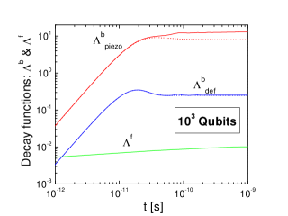
Figure 2: Maximum decay functions for $N=10^{3}$ qubits given by Eqs. (62) at zero temperature for piezo and deformation phonons and electronic baths. The constants are $g=0.03$, $\omega_{s}^{2}=10^{25}$s^-2, $\eta=9.3\cdot 10^{-8}$, $c_{L}=5\cdot 10^{3}$m/s, $q_{0}$=50nm, $d=400$nm, $\omega_{c}^{b}=\omega_{q}=5\cdot 10^{10}$s^-1 (phonons), and $\omega_{c}^{f}=1.3\cdot 10^{15}$s^-1 (electronic bath). The corresponding dotted lines are $2NQ_{2}^{0,piezo}$ and $2NQ_{2}^{0,def.}$, which illustrate the expressions for a single qubit.

We evaluate $\Lambda^{b}$, $\Lambda^{f}$ and $Q_{2}^{r}$ using Eqs. (62), (46)-(47), (67)-(68), and (57) for typical values of a multiple coupled quantum dots system imbedded in GaAs/AlGaAs for the case where we have $N=10^{3}$ qubits. The results are shown in Fig. 2. The cut-off frequency is important, since it defines a characteristic time scale. For the electron-phonon coupling the relevant phonon frequency is given by the smallest extent of the electronic wave function in the quantum dot, which we assume to be $\lambda_{0}$=100 nm. Hence, $\omega_{c}^{b}=c_{L}/\lambda_{0}$. This also implies that the coherence time decreases with a stronger quantum dot confinement. In contrast, $\omega_{c}^{f}$ for the electronic bath coupling is given by the Fermi energy of the gates. For lateral gates the Fermi energy is given by the two-dimensional electron system, where we assume a typical Fermi energy of 8.9 meV, which corresponds to a Fermi wavelength of 50nm. The coupling constant is given by (58), where $V_{0}$ is the charging energy of the dot, which we assume to be 1.2 meV and corresponds to a typical dot to gate separation of 100nm. This leads to $\eta=3.2\cdot 10^{-2}$. For a similar geometry but with top metallic gates, the Fermi energy is about 5.5 eV (for gold) and the charging energy is similar to the lateral gates geometry, i.e., 1.2 meV. This leads to $\eta=9.3\cdot 10^{-8}$. The values of $q_{0}$ and $d$ are relevant to recent experiments Fujisawa et al. (1998). With these parameters we obtain a decoherence function for the lateral gates (not shown in Fig. 2), which is five orders of magnitude larger than when we consider only top metallic gates (shown as $\Lambda^{f}$ in Fig. 2). Hence, we will only consider the top gate geometry in the remainder of this discussion.

The main contribution to decoherence is clearly given by the piezo phonons as was argued earlier Fujisawa et al. (1998). The coupling to the electronic leads (metallic) introduces a smaller decoherence decay and the form of its time-dependence is the same as the single qubit case (except for the prefactor). For the phonon bath, considering $N$ qubits, instead of one qubit, modifies the form of the time dependence in addition to the prefactor. The difference in behavior is illustrated by the solid and dotted lines in Fig. 2.

The small oscillations seen in the figure are reminiscent of coherence revival Raimond et al. (1997) and are most likely due to phase exchange between the qubits via the environmental bath. The saturation of $\Lambda^{b}$ at large times is similar to the saturation seen in the superohmic case of the spin boson model.Leggett et al. (1987) This saturation occurs because of the small density of low frequency modes in the spectral function. Indeed, at low frequencies, the leading order of the spectral function for piezo phonons in Eq. (67) is given by $J(\omega)\sim\omega^{3}$ (superohmic at low frequencies). Eventually, full decoherence would occur if we include the exchange of energy between the qubits and the bath ($\Delta\neq 0$). This introduces another time scale $T_{1}$ above which all coherence is lost. However $T_{1}$ is usually much longer than ${\omega_{c}^{b}}^{-1}$, the typical time-scale of the decoherence due to quantum fluctuations. We leave the discussion of the energy transfer processes to Section X, where we consider $\Delta\neq 0$.

The decoherence time due to the quantum and thermal fluctuations (non-dissipative) can be obtained from Eq. (62) and is given by $\Lambda^{b}(t_{dec})\simeq 1$. Hence, from Fig. 2 we can estimate that $t_{dec}\simeq$ 5ps for $N=10^{3}$ qubits at zero temperature. The temperature dependence of the decay function $\Lambda^{b}$ (Eq. (62)) for the coupling to the dominant piezo phonons is shown in Fig. 3 for $t$=1, 10, and 100ps. As expected, the main effect of an increasing temperature is to increase the decay function. At low temperatures the decay function saturates close to 100mK and the decoherence mechanism is only due to quantum fluctuations. It is interesting to note that for a small number of qubits, for example $N=10$, the decoherence function at 1ns is only 10%, which means that there is very little decoherence. However, this small decoherence would still lead to an error rate during a quantum operation.Fedichkin and Fedorov (2004)

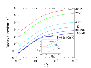
Figure 3: Time dependence of $\Lambda^{b}_{piezo}$ (Eq. (62)) for piezo phonons and $N=10^{3}$ qubits for different values of the temperature. Inset: Temperature dependence of $\Lambda^{b}_{piezo}$ for 1, 10 and 100ps. The corresponding dotted lines are the functions $2NQ_{2}^{0,piezo}$.

The temperature dependence of the decoherence function for a single qubit, which is described by the function $Q_{2}^{0,piezo}$, is shown in the inset of Fig. 3 in dotted lines. This shows that the overall dependence is similar at low temperatures and small times, where $2NQ_{2}^{0}$ is actually a good approximation to $\Lambda^{b}$. For higher temperatures and longer times the exact expressions (62)-(63) have to be used. In Fig. 4 we plot the functions $Q_{1}^{r}$ and $Q_{2}^{r}$ from Eq. (46) for the first values of $r$. Hence, in practice, it is enough to sum over a few values of $r$ in order to calculate $\Lambda^{b}$. For the phase function $X^{b}$ and $Q_{1}^{r}$ the situation is very similar.

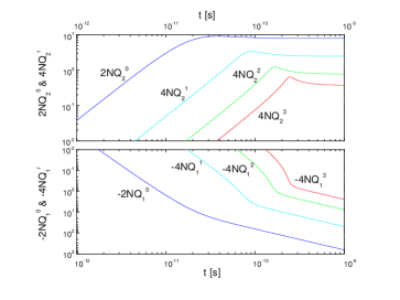
Figure 4: The functions $2NQ_{1}^{0}$, $2NQ_{2}^{0}$, $4NQ_{1}^{r}$ and $4NQ_{2}^{r}$ for piezo phonons and $r=1,2,3$ and $N=10^{3}$.

X Dynamics in the register

In previous sections VIII and IX the results were obtained assuming that no quantum operations are performed (i.e. $\Delta=0$). In this section we introduce non-trivial dynamics in order to study the effects of quantum operations on the decoherence rates.

We assume that $\Delta$ is constant. Suppose that for a set $\Xi$ of qubits, the dynamic is trivial (i.e. the quantum operation does not involve those qubits). We take $(\xi,\chi)$ to be a given path occurring in Eq. (11). Define $\xi^{tr}$ as $\xi^{tr}_{n}=0$ if $n$ is not in $\Xi$, and $\xi^{tr}_{n}=\xi_{n}(0)$ otherwise, and $\xi^{dy}$ as $\xi-\xi^{tr}$. Define $\chi^{tr}$ and $\chi^{dy}$ in the same way. The subscript $\ {}^{tr}$ stands for “trivial”, and $\ {}^{dy}$ for “dynamical”. Then, we find that the influence functionals for bosons and fermions depending only on the trivial part of the path are given by

$$\begin{array}[]{ll}\Lambda^{b,f}_{tr}&\displaystyle=\langle\xi^{tr}|Q_{2}^{b,f}(t)|\xi^{tr}\rangle\\[5.69054pt] X^{b,f}_{tr}&\displaystyle=\langle\xi^{tr}|Q_{1}^{b,f}(t)|\chi^{tr}\rangle\,.\end{array}$$ (69)

Note that since $Q_{1}^{f}(t)$ is a diagonal matrix, $X^{f}_{tr}=0$.

We now define $\overline{Q}^{b,f}_{1,2}$ as the off-diagonal part of $Q^{b,f}_{1,2}$. By definition, we have $\langle\xi^{tr}|\xi^{dy}\rangle=0$. As a consequence, we find that the part of $X^{b}$ depending on cross terms between the trivial and the dynamical parts of the path is given by

$$\begin{array}[]{l}\displaystyle x^{b}=\sum_{j=1}^{p+1}\langle\xi^{dyj}|\overline{Q}_{1}^{b}(t_{{}_{j}})-\overline{Q}_{1}^{b}(t_{{}_{j-1}})|\chi^{tr}\rangle\\ \displaystyle\hskip 17.07182pt+\langle\xi^{tr}|\overline{Q}_{1}^{b}(t-t_{{}_{j-1}})-\overline{Q}_{1}^{b}(t-t_{{}_{j}})|\chi^{dyj-1}\rangle\,,\end{array}$$ (70)

whereas $x^{f}=0$ since $Q_{1}^{f}$ is a diagonal matrix. The corresponding term for $\Lambda^{b}$, which we denote by $\lambda^{b}$, is given by the same formula with $\chi^{tr}$, $\chi^{dyj-1}$ and $\ {}_{1}$ replaced by $\xi^{tr}$, $\xi^{dyj}$, and $\ {}_{2}$ respectively. For the same reason as above, $\lambda^{f}=0$. We are interested in the dynamics of the register’s reduced density matrix for time scales smaller than the decoherence time, which we have estimated in the previous section ($t\leq t_{dec}$). As a consequence, since for $t\leq t_{dec}$, $Q_{1}^{r}(t)$ and $Q_{2}^{r}(t)$ are essentially zero for all $r\geq 1$ (see Fig. 4), we can neglect the cross terms of the bosonic influence functional, that is we can safely assume that $x^{b}=0$ and $\lambda^{b}=0$.

In general, a quantum computation can be achieved by successive single-qubit and C-NOT operations. For C-NOT gates, we consider the set-up proposed in Ref. Tanamoto (2000), described by the Hamiltonian

$$-\Delta{1-\sigma_{z}\over 2}\otimes\sigma_{x}-\varepsilon{1+\sigma_{z}\over 2}\otimes\sigma_{z}\,,$$ (71)

where a NOT operation is achieved on the right qubit after a period given by $\Delta T_{not}={\pi\over 2}$, whenever the left qubit is in the state $|-1\rangle$. Note that in a semiconductor charge quantum register, only C-NOT operations between nearest qubits can be achieved. For single-qubit gates, we consider the Hamiltonian $-\Delta\sigma_{x}-\varepsilon\sigma_{z}$. Three single-qubit operations are needed for a quantum computation. Two of them are trivial, i.e. $\Delta=0$ and $T_{1}\varepsilon=3\pi/4$ and $T_{2}\varepsilon=7\pi/8$. The last one is the Hadamar gate given by $\Delta=\varepsilon$ and $T_{Had}\sqrt{\Delta^{2}+\varepsilon^{2}}={\pi\over 2}$.

As a consequence, the decay rate of the most off-diagonal terms of the register’s density matrix for a single C-NOT operation or qubit rotation, will remain proportional to $N$. For parallel qubit rotations or C-NOT operations, the compact formulas for the bosonic influence functional are a good starting point to discuss a generalized NIBA approximation. However, a more detailed analysis is beyond the scope of this article.

XI Conclusion

We have analyzed the decoherence process in a solid state quantum register with $N$ qubits. We showed that the decay rate of the most off-diagonal terms of the register’s density matrix is proportional to $N$ in all situations relevant to a scaled charge solid-state quantum computer, where the qubits are coupled to a common phonon bath and to independent electronic gates. We obtained compact expressions for the $N$-qubit decoherence functions and argued that when performing quantum operations the decoherence function follows a very similar dependence as compared to the static case.

B.I. acknowledges support from the Swiss National Science Foundation and M.H. support from NSERC, FCAR and RQMP.

References

Shor (1997)
P. W. Shor,
SIAM J. Comput. 26,
1484 (1997).
Dubé and Stamp (2001)
M. Dubé and
P. C. E. Stamp,
Chem. Phys. 268,
257 (2001).
Shor (1995)
P. W. Shor,
Phys. Rev. A 52,
R2493 (1995).
Bennett et al. (1996)
C. H. Bennett,
D. P. DiVincenzo,
J. A. Smolin,
and W. K.
Wootters, Phys. Rev. A
54, 3824 (1996).
Palma et al. (1996)
G. M. Palma,
K.-A. Suominen,
and A. K. Ekert,
Proc. Roy. Soc. London Ser. A
452, 567 (1996).
Reina et al. (2002)
J. H. Reina,
L. Quiroga, and
N. F. Johnson,
Phys. Rev. A 65,
032326 (2002).
Hayashi et al. (2003)
T. Hayashi,
T. Fujisawa,
H. D. Cheong,
Y. H. Jeong, and
Y. Hirayama,
Phys. Rev. Lett. 91,
226804 (2003).
Tanamoto (2000)
T. Tanamoto,
Phys. Rev. A 61,
022305 (2000).
Krasheninnikov and Openov (1996)
A. V. Krasheninnikov
and L. A.
Openov, JETP Lett.
64, 231 (1996).
Brum and Hawrylak (1997)
J. A. Brum and
P. Hawrylak,
Superlattices Microstruct. 22,
431 (1997).
Bandyopadhyay et al. (1998)
S. Bandyopadhyay,
A. Balandin,
V. P. Roychowdhury,
and F. Vatan,
Superlattices Microstruct. 23,
445 (1998).
Zanardi and Rossi (1998)
P. Zanardi and
F. Rossi,
Phys. Rev. Lett. 81,
4752 (1998).
Balandin and Wang (1999)
A. Balandin and
K. L. Wang,
Superlattices Microstruct. 25,
509 (1999).
Sanders et al. (1999)
G. D. Sanders,
K. W. Kim, and
W. C. Holton,
Phys. Rev. A 60,
4146 (1999).
Openov (1999)
L. A. Openov,
Phys. Rev. B 60,
8798 (1999).
Biolatti et al. (2000)
E. Biolatti,
R. C. Iotti,
P. Zanardi, and
F. Rossi,
Phys. Rev. Lett. 85,
5647 (2000).
Fedichkin et al. (2000)
L. Fedichkin,
M. Yanchenko,
and K. A.
Valiev, Nanotechnology
11, 387 (2000).
Openov and Bychkov (1998)
L. Openov and
A. Bychkov,
Phys. Low-Dim. Struct. 9/10,
153 (1998),
cond-mat/9809112.
Leggett et al. (1987)
A. J. Leggett,
S. Chakravarty,
A. T. Dorsey,
M. P. A. Fisher,
A. Garg, and
W. Zwerger,
Rev. Mod. Phys. 59,
1 (1987).
Weiss (1999)
U. Weiss,
Quantum Dissipative Systems,
vol. 10 of Series in Modern
Condensed Matter Physics (World Scientific,
Singapore, 1999).
Prokof’ev and Stamp (2000)
N. V. Prokof’ev
and P. C. E.
Stamp, Rep. Prog. Phys.
63, 669 (2000).
Chang and Chakravarty (1985)
L. D. Chang and
S. Chakravarty,
Phys. Rev. B 31,
154 (1985).
Fröhlich (1954)
H. Fröhlich,
Adv. Phys. 3,
325 (1954).
Dubé and Stamp (1998a)
M. Dubé and
P. C. E. Stamp,
J. Low Temp. Phys. 113,
1079 (1998a).
Brandes and Kramer (1999)
T. Brandes and
B. Kramer,
Phys. Rev. Lett. 83,
3021 (1999).
Fedichkin and Fedorov (2004)
L. Fedichkin and
A. Fedorov,
Phys. Rev. A 69,
032311 (2004).
Dubé and Stamp (1998b)
M. Dubé and
P. C. E. Stamp,
Int. J. Mod. Phys. B 12,
1191 (1998b).
Fedichkin et al. (2004)
L. Fedichkin,
A. Fedorov, and
V. Privman,
Physics Letters A 328,
87 (2004).
Fujisawa et al. (1998)
T. Fujisawa,
T. H. Oosterkamp,
W. G. van der Wiel,
B. W. Broer,
R. Aguado,
S. Tarucha, and
L. P. Kouwenhoven,
Science 282,
932 (1998).
Brandes and Vorrath (2002)
T. Brandes and
T. Vorrath,
Phys. Rev. B 66,
075341 (2002).
Bruus et al. (1993)
H. Bruus,
K. Flensberg,
and H. Smith,
Phys. Rev. B 48,
11144 (1993).
Raimond et al. (1997)
J. M. Raimond,
M. Brune, and
S. Haroche,
Phys. Rev. Lett. 79,
1964 (1997).