Quantum Phase Transition of Ground-state Entanglement in a Heisenberg Spin Chain Simulated in an NMR Quantum Computer

Abstract

Using an NMR quantum computer, we experimentally simulate the quantum phase transition of a Heisenberg spin chain. The Hamiltonian is generated by a multiple pulse sequence, the nuclear spin system is prepared in its (pseudo-pure) ground state and the effective Hamiltonian varied in such a way that the Heisenberg chain is taken from a product state to an entangled state and finally to a different product state.

Quantum mechanical systems are known to undergo phase transitions at zero temperature when a suitable control parameters in its Hamiltonian is varied Sacbook . At the critical point where the quantum phase transition (QPT) occurs, the ground state of the system undergoes a qualitative change in some of its properties Sacbook . Osterloh et al. Ost02 showed that in a class of one-dimensional magnetic systems, the QPT is associated with a change of entanglement, and that the entanglement shows scaling behavior in the vicinity of the transition point. This behavior was discussed in detail for the Heisenberg model Osb02 and for the Hubbard model Gu04 . It is believed that the ground-state entanglement also plays a crucial role in other QPTs, like the change of conductivity in the Mott insulator-superfluid transition Gebbook and the quantum Hall effect Lau83 . Many of the relevant features, like the transition from a simple product state to a strongly entangled state, occur over a wide range of parameters and persist for infinite systems as well as for systems with as few as two spins AZW ; Kam02 . These systems, especially the Heisenberg spin model, are central both to condensed-matter physics and to quantum information theory. In quantum information processing, the Heisenberg exchange interaction has been shown to provide a universal set of gates Ima99 ; Rau01 and in quantum communication, information can be propagated through a Heisenberg spin chain Bos03 .

While some Heisenberg models can be solved analytically, others can only be simulated numerically. Like for other quantum systems, such simulations are extremely inefficient if the system contains more than 10-20 spins. It was therefore suggested that such simulations could be more efficiently performed on a quantum computer Fey82 . In this Letter, we discuss the simulation of a Heisenberg spin chain by an NMR quantum computer. By varying the strength of the magnetic field, we take the system, which is in the quantum mechanical ground state, through the QPT and measure the change in entanglement by quantum state tomography. The NMR techniques that we use here are closely related to earlier work where they were used to demonstrate quantum algorithms, quantum error correction, quantum simulation, quantum teleportation and more(see, e.g., Ref. NMRQC and references cited therein).

The simplest system that exhibits this behavior consists of two spins coupled by the Ising interaction

$$H=\frac{\omega_{z}}{2}(\sigma^{1}_{z}+\sigma^{2}_{z})+J_{I}\sigma^{1}_{z}\sigma^{2}_{z},\quad\quad J_{I}>0,$$ (1)

where $\sigma^{i}_{z}$ are the Pauli operators, $\omega_{z}$ a magnetic field strength, and $J_{I}$ is a spin-spin coupling constant.

In the range $-J_{I}\leq\omega_{z}\leq J_{I}$, the ground state of this system is two-fold degenerate. To avoid this complication, we add a small transverse magnetic field. The resulting Hamiltonian is

$$H=\frac{\omega_{z}}{2}(\sigma_{z}^{1}+\sigma_{z}^{2})+\frac{\omega_{x}}{2}(\sigma_{x}^{1}+\sigma_{x}^{2})+J_{I}\sigma_{z}^{1}\sigma_{z}^{2},$$ (2)

which is nondegenerate. The transverse field will always be kept small, $|\omega_{x}|\ll|\omega_{z}|,|J_{I}|$.

A symmetry-adapted basis that is an eigenbasis for vanishing transverse field ($\omega_{x}=0$) is {$\left|\uparrow\uparrow\right\rangle,\left|\Psi^{+}\right\rangle,\left|\downarrow\downarrow\right\rangle,\left|\Psi^{-}\right\rangle\}$, with $\left|\Psi^{\pm}\right\rangle=\frac{1}{\sqrt{2}}(\left|\uparrow\downarrow\right\rangle\pm\left|\downarrow\uparrow\right\rangle)$ and $\left|\downarrow\right\rangle$ and $\left|\uparrow\right\rangle$ the spin-down ($m=-\frac{1}{2}$) and spin up ($m=+\frac{1}{2}$) states. Furthermore, it is convenient to define dimensionless field strengths $g_{x}=\frac{\omega_{x}}{2J}$ and $g_{z}=\frac{\omega_{z}}{2J}$.

Since the ground state of this system is always one of the triplet states, and transitions to the singlet state are symmetry-forbidden, we can reduce our system of interest to the triplet states. For small transverse fields, $g_{x}\ll 1$, the longitudinal field $g_{z}$ determines the ground state

$$\left|\psi_{1}\right\rangle\simeq\left\{\begin{array}[]{l}\left|\uparrow\uparrow\right\rangle\hskip 19.91684ptg_{z}<-1\\ \left|\Psi^{+}\right\rangle\hskip 19.91684pt-1<g_{z}<1\\ \left|\downarrow\downarrow\right\rangle\hskip 19.91684ptg_{z}>1\end{array}\right..$$ (3)

$g_{z}=\pm 1$ are therefore quantum critical points, where the ground state changes from the ferromagnetically ordered high field states to the entangled, antiferromagnetic low-field state.

For the full system, including the transverse field, the eigenstates and eigenvalues of the three-state system are

$$\begin{array}[]{l}|\psi_{i}\rangle=\frac{1}{\sqrt{M_{i}}}(\frac{\xi_{i}^{2}+2(\xi_{i}+1)g_{z}-1-2g_{x}^{2}}{2g_{x}^{2}}\left|\uparrow\uparrow\right\rangle\\ +\frac{\xi_{i}-1+2g_{z}}{\sqrt{2}g_{x}}\left|\Psi^{+}\right\rangle+\left|\downarrow\downarrow\right\rangle),(i=1,2,3)\end{array}$$ (4)

and

$$\begin{array}[]{l}{\large\varepsilon}_{1,2}=J_{I}\xi_{1,2}=J_{I}(1-2r\cos(\theta\mp\pi/3))/3\\ {\large\varepsilon}_{3}=J_{I}\xi_{3}=J_{I}(2r\cos\theta+1)/3,\end{array}$$ (5)

where $M_{i}$ are normalization constants, $r=2\sqrt{3(g_{x}^{2}+g_{z}^{2})+1}$, and $\theta=\frac{1}{3}\arccos(\frac{4(18g_{z}^{2}-9g_{x}^{2}-2)}{r^{3}})$.

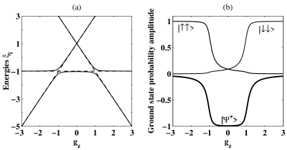
Figure 1: (a) Energy level diagram for the two-spin Heisenberg Ising model for $g_{x}=0$ (dashed lines) and $g_{x}=0.129$ (solid lines). (b) Probability amplitudes of the ground state $\left|\psi_{1}\right\rangle$ for $g_{x}=0.129$.

Figure 1 shows numerical values for the energies and the coefficients of the ground state as a function of the longitudinal field strength $g_{z}=\frac{\omega_{z}}{2J_{I}}$. The right hand side shows clearly that at strong fields ($|g_{z}|>1$), the ground state is a product state, while it corresponds to the entangled state $|\Psi^{+}\rangle$ for weak fields.

To observe the system undergoing the QPT, we simulate it on an NMR quantum computer, where the quantum spins $\sigma^{i}$ are represented by nuclear spins and the Hamiltonian (2) of the Heisenberg chain is mapped into an effective Hamiltonian generated by a sequence of radio frequency (rf) pulses acting on the nuclear spin system.

The natural Hamiltonian of our two-qubit system is

$$H_{NMR}=\frac{\omega^{1}_{L}}{2}\sigma_{z}^{1}+\frac{\omega^{2}_{L}}{2}\sigma_{z}^{2}+\frac{J_{12}}{4}\sigma_{z}^{1}\sigma_{z}^{2}.$$ (6)

The $\omega^{1,2}_{L}$ represent the Larmor frequencies of the two qubits and $J_{12}$ the spin-spin coupling constant. In addition to this static Hamiltonian, we use rf pulses to drive the dynamics of the system. In the usual rotating coordinate system, the effect of rf pulses can be written as

$$H_{rf}=\frac{\omega_{rf}}{2}(\sigma_{x}^{1}+\sigma_{x}^{2})$$ (7)

where we assumed that the rf field strength is the same for both qubits.

The target Hamiltonian (2) can be created as an average Hamiltonian by concatenating small flip angle rf pulses with short periods of free evolution, $e^{-iH\tau}\simeq e^{-iH_{rf}\tau_{p}}e^{-iH_{NMR}\tau_{prec}}$, where $\tau_{p}$ is the pulse duration and $\tau_{prec}$ the length of the free evolution period. The resulting effective Hamiltonian matches the target Hamiltonian if $\omega^{1}_{L}=\omega^{2}_{L}=\frac{\tau}{\tau_{prec}}\omega_{z}$, $\tau_{p}=\frac{\omega_{x}}{\omega_{rf}}\tau$, and $\tau_{prec}=\frac{4J_{I}}{J_{12}}\tau$. While this approximation is correct to first order in $\tau$, the symmetrized sequence

$$(H_{rf},\frac{\tau_{p}}{2})-(H_{NMR},\tau_{prec})-(H_{rf},\frac{\tau_{p}}{2})$$ (8)

generates the desired evolution to second order in $\tau$. Figure 2 shows the sequence of rf pulses required to generate this evolution.

.

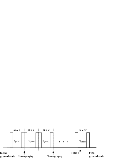
Figure 2: Sequence of rf pulses applied to both spins to simulate the target Hamiltonian. The boxes represent pulses that induce rotations around the x-axes of the rotating frame, the separations between them the free precession periods. The index $m$ for the different periods runs from $0$ to $M$.

To prepare the system in the ground state, we use the technique of pseudo-pure states pps : we prepare a density operator $\rho_{pp}(\psi_{1})=\frac{1}{tr(\mathbf{1})}\mathbf{1}+\alpha|\psi_{1}\rangle\langle\psi_{1}|$. Here, $\mathbf{1}$ is the unity operator and $\alpha$ a small constant of the order of $10^{-5}$. To measure the order parameter (entanglement), we apply quantum state tomography qst . The system can then be taken through the phase transition by adiabatically changing the magnetic field $g_{z}$ of the effective Hamiltonian, which acts as a control parameter.

To ensure that the system always stays in the ground state, the variation of the control parameter has to be sufficiently slow, so that the condition $\left|\frac{\langle\psi_{1}(t)\left|\dot{\psi}_{e}(t)\right\rangle}{\varepsilon_{e}(t)-\varepsilon_{1}(t)}\right|\ll 1$ is fulfilled, where the index $e$ refers to the excited states Messbook . Choosing $g_{z}$ as the control parameter, we write the adiabaticity condition as

$$\left|\frac{dg_{z}}{dt}\right|\ll J_{I}^{2}\chi=J_{I}^{2}\left|\frac{(\xi_{2}(t)-\xi_{1}(t))^{2}}{\langle\psi_{1}(t)|\frac{\partial H}{\partial g_{z}}|\psi_{2}(t)\rangle}\right|,$$ (9)

where the dimensionless parameter $\chi$ quantifies the sensitivity to the control parameter $g_{z}$ and we have concentrated on the first excited state $|\psi_{2}\rangle$, which is the critical one for transitions from the ground state.

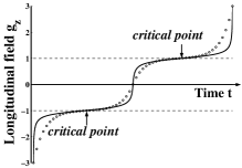
Figure 3: Adiabatic magnetic field sweeps $g_{z}(t)$. The solid line was calculated for constant adiabaticity parameter $\frac{\chi}{dg_{z}/dt}$ (see equ. (9)) for a transverse field $g_{x}=0.129$; the circles represent the values obtained from the numerical optimisation of the discretised scan.

Equation (9) defines the optimal sweep of the control parameter $g_{z}(t)$, with the scan speed $\left|\frac{dg_{z}}{dt}\right|\propto\chi$. Figure 3 shows the required time dependence of the magnetic field. The resulting transfer is therefore highest for a given scan time or the scan time minimised for a required adiabaticity.

The experimental implementation generates an effective Hamiltonian that is constant for a time $\tau$ (see equ. (8)). For this stepwise approximation, the duration of each time step has to be chosen such that (i) the time is short enough that the average Hamiltonian approximation holds and (ii) the adiabaticity criterion remains valid. While this calls for many short steps, there is also a lower limit for the duration of each step, which is dictated by experimental aspects: switching transients, which are not taken into account in the Hamiltonian of equ. (8), tend to generate errors that increase with the number of cycles.

We used a numerical optimisation procedure to determine the optimal sequence of Hamiltonians, taking the full level structure into account. Choosing a hyperbolic sine as the functional form, we optimised its parameters and found the optimised discrete scan represented by the circles in Fig. 3.

To determine the optimal number of steps, we used the same numerical simulation, keeping the functional dependence $g_{z}$ vs. $t$ constant, but increasing the number of steps. The results are summarized in Fig. 4, which plots the lowest fidelity encountered during each scan against the number of steps taken in the simulation. The fidelity is calculated as the overlap of the state with the ground state at the relevant position. The simulation shows also the effect of decoherence, which reduces the achievable fidelity if the total duration of the scan becomes comparable to the decoherence time. The model that we used to take the effect of decoherence into account is similar to that of Vandersypen et al shor .

.

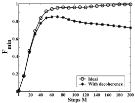
Figure 4: Numerical simulation of the minimum fidelities during the adiabatic passage vs. number of steps with ($*$) and without ($\bigcirc$) decoherence effects.

For the experimental implementation, we used the ¹³C and ¹H spins of ¹³C_labeled chloroform (both spins 1/2). The relatively large spin-spin coupling constant of $\frac{J_{12}}{2\pi}$=214.94Hz makes this molecule well suited for this experiment. The chloroform was diluted in acetone-d₆ and experiments were carried out at room temperature on a Bruker DRX-500 MHz spectrometer. The pseudo-pure initial state $\rho_{pp}(\uparrow\uparrow)$ was generated by spatial averaging pps . The fidelity of this state preparation was checked by quantum state tomography and found to be better than 0.99.

The adiabatic scan through the QPT was achieved by shifting the rf frequencies of both channels by the same amount after each period. Using the sweep $g_{z}(t)$ shown in Fig. 3, the offset was changed from $g_{z}=-3$ to $g_{z}=+3$ in 60 steps. The evolution of the system during the scan was checked by performing a complete quantum state tomography after every second step during the experiment.

As a quantitative measure of the QPT, we used the concurrence as the order parameter, which is related to ”the entanglement of formation” Wootters and ranges form 0 (no entanglement) to 1 (maximum entanglement). For this purpose, we calculated the concurrence C from the tomographically reconstructed deviation density matrices $\rho$ as $C(\rho)=max\{\lambda_{1}-\lambda_{2}-\lambda_{3}-\lambda_{4},0\}$, where $\lambda_{i}(i=1,2,3,4)$ are the square roots of the eigenvalues of $\rho(\sigma^{1}_{y}\sigma^{2}_{y})\rho^{*}(\sigma^{1}_{y}\sigma^{2}_{y})$ in decreasing order.

.

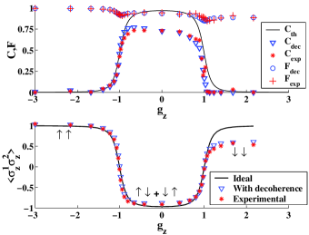
Figure 5: (Color online)(a) Measured fidelity $F_{\exp}$ ($+$) and concurrence $C_{\exp}$ ($*$) compared to the concurrence calculated for an ideal scan $C_{th}$ (solid line) and the simulated concurrence $C_{dec}$ ($\bigtriangledown$) and fidelity $F_{dec}$ ($\bigcirc$) when decoherence is taken into account. (b) Measured values ($*$) of the two-spin correlaror $\left\langle\sigma_{z}^{1}\sigma_{z}^{2}\right\rangle$ compared to the theoretical (solid line) and simulated values with decoherence($\bigtriangledown$).

Figure 5(a) shows the measured concurrence $C_{\exp}=C(\rho_{\exp})$ as individual points and compares them with the theoretical values $C_{th}$. Both data sets clearly show the expected QPTs near the critical points $g_{z}=\pm 1$. The entangled ground state for $|g_{z}|<1$ is characterised by a concurrence close to 1, while the high field states are only weakly entangled (the entanglement vanishes for $g_{x}=0$).

The experimentally determined concurrence remains below $\sim 0.75$, significantly less than the theoretical values. To verify that this deviation is due to decoherence, we simulated the experiment, taking into account the details of the pulse sequence as well as the effect of decoherence. We obtained good agreement between theoretical and experimental data if we assumed a total decoherence time of 130 ms, which is slightly longer than the 110 ms scan time used in the experiment. Fig.5(a) shows the simulated values of the concurrence as triangles; their evolution during the scan is quite similar to that of the experimental data points.

To assess the quality of the adiabatic scan, we also determined the fidelities $F_{\exp}=F(\rho_{\exp})$ from the tomographically reconstructed density operators. The fidelities, which are shown at the top of Fig.5(a), deviate from unity when the system passes through the critical points and shows some overall decrease due to decoherence. Again, the simulated fidelities agree remarkably well with the experimental values.

As a second order parameter, we also determined the two-spin correlation Sacbook $\left\langle\sigma_{z}^{1}\sigma_{z}^{2}\right\rangle=Tr(\rho_{\exp}\sigma_{z}^{1}\sigma_{z}^{2})$, which are shown in Fig.5(b). As expected, the system is ferromagnetically ordered ($\left\langle\sigma_{z}^{1}\sigma_{z}^{2}\right\rangle=+1$) at high fields, but turns to an antiferromagnetic state ($\left\langle\sigma_{z}^{1}\sigma_{z}^{2}\right\rangle=-1$) at low fields between the two quantum critical points. Comparing Fig. 5(a) with (b), the concurrence has the similar behavior to the two-spin correlation.

In conclusion, we have discussed an experimental quantum simulation of a quantum phase transition in a Heisenberg spin chain. Heisenberg spin chains, which have been investigated in detail in solid state physics, play an important role in a number of proposed solid state quantum computers. During the course of the simulation, the system ground state changes from a classical product state to an entangled state and back to another product state. Like in many other proposed quantum simulations, this system had to be swept adiabatically through the relevant parameter space by properly varying a Hamiltonian parameter. The techniques developed here may also be useful for other types of adiabatic quantum computing which have been proved to be effective for NP-hard problems Lato2004 , e.g., the classically NP-hard ground state search. Furthermore, the adiabatic passage can provide a novel method to create entanglement Una01 . The simulation can be extended to other types of Heisenberg spin chains, e.g., Heisenberg XY or XYZ models etc.; work in this direction is under way.

We thank Dr. X. Zou and Dr. C. Lee for helpful discussions. The experiments were performed at the Interdisciplinary Center for Magnetic Resonance. X. P. is supported by the Alexander von Humboldt Foundation. J. D. acknowledges the support from NUS Research Project (Grant No.R-144-000-071-305) and National Fundamental Research Program (Grant No. 2001CB309300).

References

- (1) S. Sachdev, Quantum Phase Transition (Cambridge University Press, Cambrige 1999).
- (2) A. Osterloh, L. Amico, G. Falci and R. Fazio, Nature 416, 608 (2002).
- (3) T. J. Osborne and M. A. Nielsen, Phys. Rev. A 66, 032110 (2002); J. Vidal, G. Palacios and R. Mosseri, ibid. 69, 022107 (2004); G. Vidal, J. I. Latorre, E. Rico and A. Kitaev, Phys. Rev. Lett. 90, 227902 (2003); F. Verstraete, M. Popp and J. I. Cirac, Phys. Rev. Lett. 92, 027901 (2004); J. I. Loutorre, E. Rico and G. Vidal,e-print quant-ph/0304098;
- (4) S. J. Gu, S. S. Deng, Y. Q. Li and H. Q. Lin, e-print quan-ph/0405067.
- (5) F. Gebbhard, The Mott Metal-Insulator Transition: Models and Methods (Springer-Verlag, New York, 1997).
- (6) R. B. Laughlin, Phys. Rev. Lett. 50, 1395 (1983).
- (7) M. C. Arnesen, S. Bose and V. Vedral, Phys. Rev. Lett. 87, 017901 (2001); L.Zhou, H. S. Song, Y. Q. Guo and C. Li, Phys. Rev. A 68, 024301 (2003); X. Wang, ibid 66, 034302 (2002).
- (8) G. L. Kamta and A. F. Starace, Phys. Rev. Lett. 88, 107901 (2002);
- (9) A. Imamoglu, D. D. Awschalom, G. Burkard, F. P. DiVincenzo, D. Loss, M. Sherwin and A. Small, Phys. Rev. Lett. 83, 4204.(1999).
- (10) R. Raussendorf and H. J. Briegel, Phys. Rev. Lett. 86, 5188 (2001).
- (11) S. Bose, Phys. Rev. Lett. 91, 207901 (2003); V. Subrahmanyam, Phys. Rev. A 69, 034304 (2004).
- (12) R. P. Feynman, Int. J. Theor. Phys. 21, 467 (1982).
- (13) L. M. K. Vandersypen and Isaac L. Chuang, e-print quant-ph/0404064.
- (14) D. G. Cory, A. F. Fahmy and T. F. Havel, Proc. Natl. Acad, Sci. USA, 94, 1634(1997); N. A. Gershenfeld and I. L. Chuang, Science, 275, 350 (1997) .
- (15) L. M. K. Vandersypen, M. Steen, M. H. Sherwood, C. S. Yannoni, G. Breyta and I. L. Chuang, Appl. Phys. Lett. 76, 646 (2000).
- (16) A. Messiah, Quantum Mechanics (Wiley, New York, 1976).
- (17) L. M. K. Vandersypen, M. Steffen, G. Breyta, C. S. Yannoni, M. H. Sherwood and I. L. Chuang, Nature (London) 414, 883 (2001).
- (18) W.K. Wootters, Phys. Rev. Lett. 80, 2245 (1998).
- (19) E. Farhi, J. Goldstone, S. Gutmann, J. Lapan, A. Lundgren and D. Preda, Science 292, 472 (2001); M. Steffen, W. vanDam, T. Hogg, G. Breyta and I. Chuang, Phys. Rev. Lett. 90, 067903 (2004); J. I. Latorre and R. Orus, Phys. Rev. A 69, 062302 (2004).
- (20) R. G. Unanyan, N. V. Vitanov and K. Bergmann, Phys. Rev. Lett. 87, 137902 (2001); N. F. Bell, R. F. Sawyer, R. R. Volkas and Y. Y. Y. Wong, Phys. Rev. A 65, 042328 (2002).