Experimental creation of entanglement using separable state

Abstract

We experimentally demonstrate the entanglement can be created on two distant particles using separate state. We show that two data particles can share some entanglement while one ancilla particle always remains separable from them during the experimental evolution of the system. Our experiment can be viewed as a benchmark to illustrate the idea that no prior entanglement is necessary to create entanglement.

I Introduction

Entanglement is one of the inherent features of quantum mechanics epr . It is unambiguously a crucial resource and also plays an important role in most of quantum information processing (QIP) tasks, e.g., bennett1 ; bennett2 . It becomes well worth investigating how entanglement is available.

There have been several proposals to create entanglement. (i) Applying a global quantum operation on the interested system barenco . For simplicity, we consider the initial state is the ground state $\left|00\ldots 0\right\rangle$ in an $N$-qubit system. The entangled state $(\left|00\ldots 0\right\rangle+\left|11\ldots 1\right\rangle)/\sqrt{2}$ can be created by a Hadamard gate followed by $(N-1)$ controlled-not (CNOT) gates. Based on this idea, the three-qubit Greenberger-Horne-Zeilinger (GHZ) state was generated experimentally lafla . Recently, Zhou et al. zhou proposed an evolution method to create multi-qubit maximally entangled state in the nuclear magnetic resonance (NMR) model, and their method need only a single-step operation. Note that such kind of methods requires the interaction between the particles. However, this direct interaction is not always existing in a real physical system. Therefore, we should consider the situation under the separated condition. (ii) Making use of the swap operation madi . The basic idea is that firstly entangling two ancilla particles which are directly interacted, and then transferring this entanglement to another pair of data particles which are separable via two swap gates. This method, more precisely speaking, can be called as entanglement transfer. Recently Boulant et al. boulant1 have demonstrated this idea on a four-qubit liquid NMR quantum processor. (iii) Distributing entanglement using a separable state. This idea was proposed by Cubbit et al. cubitt . They show that no prior entanglement is necessary to create entanglement.

A few of comments about the differences between the method (iii) and the former two are in order. First, the method (iii) can be used in the situation where there are no direct interactions among the particles, which is the difference from the method (i). Second, the swap operation is not used in the method (iii), which is the difference from the method (ii). Last but not the least, the method (iii) clarifies the fact that two separable particles can be entangled without the ancilla particle ever becoming entangled with them.

In this Letter, we report an experimental creation of entanglement based on the third method mentioned above using NMR technique. The problem of interest in this Letter is the experimental demonstration of entanglement creation between two non-directly-coupled spins with the aid of one ancilla spin, and most importantly, keeping the ancilla never entangled with the data spins. Our results confirm the separable state can be used to create entanglement.

II Theory of entanglement creation using separable state

We begin with a three-particle system — A, B and C, each of which is a spin-half quantum bit (qubit). Suppose the two data qubits A and B are so well isolated or far away over a long distance that they do not directly interact with each other, while ancilla C interacts with both A and B. Our goal is to entangle A and B, or at least entangle them with some probability. An explicit case cubitt is given as follows.

The initial state $\rho_{0}$ is well chosen to satisfy the condition that the system ABC is separable at the first beginning and can finally lead to the entangled state in AB system after some certain quantum operations. We choose $\rho_{0}$ as a mixed state composed of the six pure ones (note that the pure state in ABC is impossible to achieve our goal cubitt ),

$$\rho_{0} =\frac{1}{6}P[\frac{1}{\sqrt{2}}\left(\left|0\right\rangle+\left|1\right\rangle\right)\otimes\frac{1}{\sqrt{2}}\left(\left|0\right\rangle+\left|1\right\rangle\right)\otimes\left|0\right\rangle]$$

$$+\frac{1}{6}P[\frac{1}{\sqrt{2}}\left(\left|0\right\rangle+i\left|1\right\rangle\right)\otimes\frac{1}{\sqrt{2}}\left(\left|0\right\rangle-i\left|1\right\rangle\right)\otimes\left|0\right\rangle]$$

$$+\frac{1}{6}P[\frac{1}{\sqrt{2}}\left(\left|0\right\rangle-\left|1\right\rangle\right)\otimes\frac{1}{\sqrt{2}}\left(\left|0\right\rangle-\left|1\right\rangle\right)\otimes\left|0\right\rangle]$$

$$+\frac{1}{6}P[\frac{1}{\sqrt{2}}\left(\left|0\right\rangle-i\left|1\right\rangle\right)\otimes\frac{1}{\sqrt{2}}\left(\left|0\right\rangle+i\left|1\right\rangle\right)\otimes\left|0\right\rangle]$$

$$+\frac{1}{6}P[\left|001\right\rangle]+\frac{1}{6}P[\left|111\right\rangle],$$ (1)

where the symbol $P[\left|\varphi\right\rangle]=\left|\varphi\right\rangle\left\langle\varphi\right|$ denotes the density matrix corresponding to state $\left|\varphi\right\rangle$. From Eq. (1), A, B and C are separable from each other.

Next, apply a CNOT gate on qubits A and C, where A is the control qubit and C the target qubit. From nontrivial calculation, the initial state (1) will become as

$$\rho_{1} =\frac{1}{3}P[\left|\Phi_{GHZ}\right\rangle]+\frac{1}{6}P[\left|001\right\rangle]$$

$$+\frac{1}{6}P[\left|010\right\rangle]+\frac{1}{6}P[\left|101\right\rangle]+\frac{1}{6}P[\left|110\right\rangle],$$ (2)

where $\left|\Phi_{GHZ}\right\rangle=\frac{1}{\sqrt{2}}\left(\left|000\right\rangle+\left|111\right\rangle\right)$ is the GHZ state. Note the difference of the phases in the singlet states in the initial state (1) is counteracted after the CNOT operation. In this state, we can check cubitt that C is separable from AB, B is separable from AC, and only A is entangled with BC.

Later, send the qubit C to B through quantum channel, and then apply another CNOT gate on qubits B and C, where B is the control qubit and C the target qubit. Thus, the final state will be

$$\rho_{2}=\frac{1}{3}P[\left|\phi^{+}\right\rangle_{AB}\otimes\left|0\right\rangle_{C}]+\frac{2}{3}(\frac{1}{4}I)_{AB}\otimes\left|1\right\rangle_{C}\left\langle 1\right|],$$ (3)

where $\left|\phi^{+}\right\rangle=\frac{1}{\sqrt{2}}\left(\left|00\right\rangle+\left|11\right\rangle\right)$ is the Bell state, and $I$ is the unit matrix of order 4. From Eq. (3), C still remains separable from AB, but the entanglement between A and B is produced. Obviously, measuring C in the computational basis, the entangled state $\left|\phi^{+}\right\rangle$ of AB will be extracted with the probability 1/3. Note that the AB system after tracing out C is not an entangled state, because after tracing, AB is in a type of Werner state werner $\frac{1}{3}\left|\phi^{+}\right\rangle\left\langle\phi^{+}\right|+\frac{2}{3}\cdot\frac{I}{4}$, which is just separable.

It is well known that entanglement can be created on two distant qubits by sending a mediating (ancilla) particle between them, and many multi-qubit quantum information transmission protocols are based on this kind of entanglement creation luo ; wei . One may expect that the ancilla necessarily becomes entangled with the system. However, from the above analysis, the scheme proved that the ancilla C can never entangled with the two data qubits AB although we used the interactions between C and AB.

III Experimental demonstration

NMR is one of the most important physical system to explore the implementation of QIP experimentally, especially in the few-qubit system. NMR quantum processor has been widely used to test many kinds of QIP tasks (for a review see e.g., jones ; cory1 ). The nature of NMR quantum computing is reinvestigated recently long .

Since the nuclear spins are fixed in the molecule through chemical bonds in NMR experiment, there is a distance of only a few angstrom ($\mathring{A}$) between different spins, thus it is difficult to realize quantum channel in nuclear spin system nielsen . Our experiment made a demonstration of quantum communication, rather than a practical means for sending information through quantum channel on distant particles. The whole demonstration procedure is shown in Fig. 1.

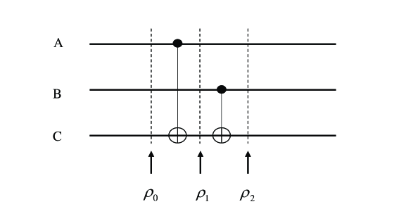
Figure 1: Quantum circuit to create entanglement between two distant qubits A and B, while qubit C works as an ancilla, which is never entangled with AB during our scheme. Time flows from left to right. $\rho_{0}$ is the initial state, $\rho_{1}$ is the state after the CNOT gate on AC, and $\rho_{2}$ is the final state after the CNOT gate on BC. For the states $\rho_{0}$, $\rho_{1}$, $\rho_{2}$, we reconstruct their density matrices.

We performed the experiment on a Bruker AVANCE 400 MHz spectrometer, keeping temperature at 300K. The spin system is ¹³C-labeled alanine $NH_{3}^{+}-C^{\alpha}H(C^{\beta}H_{3})-C^{\prime}OO^{-}$ du , where carbons $C^{\prime},C^{\beta},C^{\alpha}$ correspond to qubits A, B and C, respectively. In the following, we label the three qubits A, B, C as 1, 2, 3 in keeping with the conventional parlance. The coupling constants between three carbons are

$$J_{13}=54.2Hz,J_{23}=35.1Hz,J_{12}=-1.3Hz.$$

In our experiment, $J_{12}$ is always refocused though the coupling constant is small. This condition means that qubits 1 and 2 have no interaction which agrees with our demand. The experimental process is explained as the following three stages:

$(1)$ Prepare for the initial state as shown in Eq. (1). We firstly assemble the pseudopure state using the gradient-based spatial averaging cory2 . Note that since the NMR system is a spin ensemble, it is not easy to prepare for a pure state experimentally. However, the unitary dynamics of the pseudopure state is same as the pure state up to a certain scaling factor gershenfeld ; cory3 . The pseudopure state, keeping the traceless part, can be expressed with the product operators formalism ernst which has been commonly used in NMR community,

$$\rho_{pp} =\left|000\right\rangle\left\langle 000\right|$$ (4)

$$=I_{z}^{1}+I_{z}^{2}+I_{z}^{3}+2I_{z}^{1}I_{z}^{2}+2I_{z}^{1}I_{z}^{3}+2I_{z}^{2}I_{z}^{3}+4I_{z}^{1}I_{z}^{2}I_{z}^{3},$$

where $I_{\alpha}^{i}=\frac{1}{2}\sigma_{\alpha}^{i}$ $(i=1,2,3,\alpha=x,y,z)$, $\sigma_{\alpha}$ is the Pauli matrix.

In order to obtain the initial state from the pseudopure state, we note that the initial state (1) is a six-componential mixed state. Our scheme involves six experiments and a sum of these six results. The scheme to prepare for the initial state is shown in table 1.

Table 1: The six components in the initial state and the corresponding pulse sequences for the preparation of the initial state. In the right column, $(\theta)_{axis}^{spins}$ denote the radio frequency pulses, which are applied to the spins in the superscript, along the axis in the subscript, and by the flip angle in the bracket.

Components in the initial state	Pulse sequence
$\frac{1}{\sqrt{2}}\left(\left|0\right\rangle+\left|1\right\rangle\right)\otimes\frac{1}{\sqrt{2}}\left(\left|0\right\rangle+\left|1\right\rangle\right)\otimes\left|0\right\rangle$	$\left(\frac{\pi}{2}\right)_{y}^{1,2}$
$\frac{1}{\sqrt{2}}\left(\left|0\right\rangle+i\left|1\right\rangle\right)\otimes\frac{1}{\sqrt{2}}\left(\left|0\right\rangle-i\left|1\right\rangle\right)\otimes\left|0\right\rangle$	$\left(\frac{\pi}{2}\right)_{-x}^{1}\left(\frac{\pi}{2}\right)_{x}^{2}$
$\frac{1}{\sqrt{2}}\left(\left|0\right\rangle-\left|1\right\rangle\right)\otimes\frac{1}{\sqrt{2}}\left(\left|0\right\rangle-\left|1\right\rangle\right)\otimes\left|0\right\rangle$	$\left(\frac{\pi}{2}\right)_{-y}^{1,2}$
$\frac{1}{\sqrt{2}}\left(\left|0\right\rangle-i\left|1\right\rangle\right)\otimes\frac{1}{\sqrt{2}}\left(\left|0\right\rangle+i\left|1\right\rangle\right)\otimes\left|0\right\rangle$	$\left(\frac{\pi}{2}\right)_{x}^{1}\left(\frac{\pi}{2}\right)_{-x}^{2}$
$\left|001\right\rangle$	$\left(\pi\right)_{y}^{3}$
$\left|111\right\rangle$	$\left(\pi\right)_{y}^{1,2,3}$

The summed result corresponds to the initial state (1) , whose expression in terms of the product operators is

$$\rho_{0}=I_{z}^{3}+2I_{x}^{1}I_{x}^{2}-2I_{y}^{1}I_{y}^{2}+2I_{z}^{1}I_{z}^{2}+4I_{x}^{1}I_{x}^{2}I_{z}^{3}-4I_{y}^{1}I_{y}^{2}I_{z}^{3}-4I_{z}^{1}I_{z}^{2}I_{z}^{3}.$$ (5)

$(2)$ Apply a CNOT operation on AC. The pulse sequence for realizing the CNOT gate jones ; vander is $\left(\frac{\pi}{2}\right)_{y}^{3}-\frac{1}{2J_{13}}-\left(\frac{\pi}{2}\right)_{x}^{3}-\left(\frac{\pi}{2}\right)_{-z}^{3}-\left(\frac{\pi}{2}\right)_{z}^{1}$, where the symbol $\frac{1}{2J_{ij}}$ denotes the evolution time dominated by the J coupling between spins $i$ and $j$; $z$ pulse on spin $i$ is implemented using the combination of $x$ and $y$ pulses $\left(\frac{\pi}{2}\right)_{x}^{i}-\left(\frac{\pi}{2}\right)_{y}^{i}-\left(\frac{\pi}{2}\right)_{-x}^{i}$. During the evolution time $\frac{1}{2J_{13}}$, the refocusing pulses on spins 1 and 3 are applied to eliminate not only the coupling between B and AC, but also the effect of the chemical shift. The state after this stage is

$$\rho_{1}=2I_{z}^{1}I_{z}^{2}+2I_{z}^{1}I_{z}^{3}-2I_{z}^{2}I_{z}^{3}-4I_{y}^{1}I_{x}^{2}I_{y}^{3}-4I_{x}^{1}I_{y}^{2}I_{y}^{3}+4I_{x}^{1}I_{x}^{2}I_{x}^{3}-4I_{y}^{1}I_{y}^{2}I_{x}^{3}.$$ (6)

$(3)$ Apply another CNOT operation on BC and obtain the final state, which can be expressed as

$$\rho_{2}=-I_{z}^{3}+2I_{x}^{1}I_{x}^{2}-2I_{y}^{1}I_{y}^{2}+2I_{z}^{1}I_{z}^{2}+4I_{x}^{1}I_{x}^{2}I_{z}^{3}-4I_{y}^{1}I_{y}^{2}I_{z}^{3}+4I_{z}^{1}I_{z}^{2}I_{z}^{3},$$ (7)

where the final state includes the entanglement of AB. If performing a projective measurement on C, we can extract the entanglement on AB with probability $1/3$. However, NMR measure is a spatial ensemble average or an expected value cory1 , rather than a projective measurement. Though we can mimic the projective (strong) measurement by magnetic field gradients tekle1 or natural decoherence nielsen , these two techniques do not adapted here because both of them can not distinguish whether the measured qubit is projected into space $\left|0\right\rangle\left\langle 0\right|$ or $\left|1\right\rangle\left\langle 1\right|$. In other words, after the mimic projective measurement, the state is that of tracing out the measured qubit, but this state, as mentioned above, is not an entangled state.

As a consequence, to confirm the entanglement existing in the final state, we use the state tomography technique chuang to reconstruct the density matrices at the corresponding three experimental stages. The results are shown in Fig. 2.

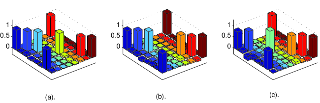
Figure 2: Real parts of the reconstructed density matrices of (a).the initial state $\rho_{0}$, (b).the medial state $\rho_{1}$, and (c).the final state $\rho_{2}$. The imaginary parts are essentially zero. The rows and columns represent the standard computational basis, with $\left|000\right\rangle$ starting from the leftmost column and $\left|111\right\rangle$ the rightmost column.

The experimental efficacy was quantified by the attenuated correlation tekle1 , which takes into account not only systematic errors in experiment, but also the random errors. This measure is given by

$$C(\rho^{exp})=\frac{Tr\left(\rho^{exp}\rho^{the}\right)}{Tr\left(\rho^{the}\rho^{the}\right)}$$ (8)

where $\rho^{the}$ is the measured pseudopure ground state (the reconstructed density matrix is not shown here); $\rho^{exp}$ represents the experimental state realized by a series of pulse sequences. The values of the correlation for the three states $\rho_{0},\rho_{1},\rho_{2}$ are $C(\rho_{0}^{exp})=98\%,C(\rho_{1}^{exp})=95\%,C(\rho_{2}^{exp})=89\%$, respectively. The correlation values show that spins 1 and 2 are separable in both $\rho_{0}$ and $\rho_{1}$, but entangled in $\rho_{2}$, while spin 3 keeps separable in $\rho_{0},\rho_{1},\rho_{2}$ by the corresponding to Eqs. (1), (2), (3). The loss of correlation mainly includes the imperfect selective pulses, and the variability during the measurement process.

IV Conclusion

We demonstrated that entanglement can be produced using separated state with NMR technique. In our scheme, there is only one ancilla qubit required to obtain the entanglement on two qubits which have no direct interaction. Compared with the entanglement swapping boulant1 where two ancilla qubits are required, the number of the ancilla is reduced. This suggests that our experimental method is less demanding on the qubit resource. On the other hand, we show that if we select a proper initial state, the ancilla qubit will never entangle with the data qubits during the evolution of the system, which is completely different form the common used method to create entanglement on distant qubits wei . This also shows a striking fact that no prior entanglement is required to create entanglement. Moreover, this scheme can be extended to multi-qubit system where there are no direct interactions among the qubits cubitt .

It should be noted that, using this method to create entanglement, a projective measurement is needed to extract the $(n-1)$-qubit entanglement from the $n$-qubit system for the aim of later QIP task. Alternatively, one also can extract the useful information from the final state after the whole QIP task according to the principle of state superposition and parallelism.

- (1) Einstein A, Podolsky B and Rosen N 1935 Phys. Rev. 47 777
- (2) Bennett C H, Brassard G, Crépeau C, Jozsa R, Peres A and Wootters W K 1993 Phys. Rev. Lett. 70 1895
- (3) Bennett C H and Wiesner S J 1992 Phys. Rev. Lett. 69 2881
- (4) Barenco A, Deutsch D, Ekert A and Jozsa R 1995 Phys. Rev. Lett. 74 4083
- (5) Laflamme R, Knill E, Zurek W H, Carasti P and Mariappan S V S 1998 Phil. Trans. R. Soc. Lond. A 356 1941
- (6) Zhou B, Tao R B and Shen S Q 2004 Phys. Rev. A 79 022311
- (7) Mádi Z L, Brüschweiler R and Ernst R R 1998 J. Chem. Phys. 109 10603
- (8) Boulant N, Fortunato E M, Pravia M A, Teklemariam G, Cory D G and Havel T F 2002 Phys. Rev. A 65 024302
- (9) Cubitt T S, Verstraete F, Dür W and Cirac J I 2003 Phys. Rev. Lett. 91 037902
- (10) Werner R F 1989 Phys. Rev. A 40 4277
- (11) Luo J, Wei D X, Xiao L and Zeng X Z 2002 Chin. Phys. Lett. 19 7
- (12) Wei D X, Luo J, Yang X D, Sun X P, Zeng X Z, Liu M L, Ding S W and Zhan M S 2004 Chin. Phys. 13 817
- (13) Jones J A 2001 Prog. NMR Spectrosc. 38 325
- (14) Cory D G, Laflamme R, Knill E, Viola L, Havel T F, Boulant N, Boutis G, Fortunato E, Lloyd S, Martinez R, Negrevergne C, Pravia M, Sharf Y, Teklemariam G, Weinstein Y S and Zurek W H 2000 Fortschr. Phys. 48 875
- (15) Long G L, Zhou Y F, Jin J Q and Sun Y 2004 Preprint quant-ph/0408079
- (16) Nielsen M A, Knill E and Laflamme R 1998 Nature 396 52
- (17) Du J F, Shi M J, Wu J H, Zhou X Y and Han R D 2001 Phys. Rev. A 63 042302
- (18) Cory D G, Price M D and Havel T F 1998 Physica D 120 82
- (19) Gershenfeld N A and Chuang I L 1997 Science 275 350
- (20) Cory D G, Fahmy A F and Havel T F 1997 Proc. Natl. Acad. Sci. USA 94 1634
- (21) Ernst R R, Bodenhausen G and Wokaun A Principles of Nuclear Magnetic Resonance in One and Two Dimensions. (Oxford University Press, Oxford, 1987).
- (22) Vandersypen L M K and Chuang I L 2004 Preprint quant-ph/0404064
- (23) Chuang I L, Gershenfeld N A, Kubinec M G and Leung D 1998 Proc. R. Soc. Lond. A 454 447
- (24) Teklemariam G, Fortunato E M, Pravia M A, Havel T F and Cory D G 2001 Phys. Rev. Lett. 86 5845