Bounds on integrals of the Wigner function: the hyperbolic case

I. Abstract

Wigner functions play a central role in the phase space formulation of quantum mechanics. Although closely related to classical Liouville densities, Wigner functions are not positive definite and may take negative values on subregions of phase space. We investigate the accumulation of these negative values by studying bounds on the integral of an arbitrary Wigner function over noncompact subregions of the phase plane with hyperbolic boundaries. We show using symmetry techniques that this problem reduces to computing the bounds on the spectrum associated with an exactly-solvable eigenvalue problem and that the bounds differ from those on classical Liouville distributions. In particular, we show that the total “quasiprobability” on such a region can be greater than 1 or less than zero.

II. INTRODUCTION

Since its introduction ¹, the Wigner function has been the subject of extensive study in the fields of quantum physics, quantum chemistry and signal analysis (see ^{2; 3; 4; 5; 6; 7; 8; 9; 10} and references therein). Since Wigner functions represent quantum states on phase space, they play a key role in the phase space formulation of quantum mechanics. They are also designed to closely resemble the joint densities of position and momentum, known as Liouville densities, that are used in classical mechanics. In quantum physics, such studies have been stimulated in recent times by the development of quantum tomography, which has enabled the reconstruction of Wigner functions corresponding to states of a variety of quantum systems ¹¹. Such experimental observations have confirmed that Wigner functions can be negative on subregions of phase space. This is one of several properties that can be used to distinguish Wigner functions from classical Liouville densities.

The study of these “quantum properties” has been approached in a number of ways including calculations of pointwise bounds on Wigner functions and bounds on various moments ^{12; 13; 14; 15; 16}. A more recent development has been the study of bounds on integrals of the Wigner function over subregions of the phase space ^{17; 18; 19}, which we denote by $\Gamma$ . We call such integrals quasiprobability integrals (qpis). For a given subregion $S$ of $\Gamma$, the problem of determining best possible upper and lower bounds on all possible qpi’s over $S$ has been shown to be equivalent to the problem of determining the supremum and infimum of the spectrum of the region operator associated with $S$. This operator is just the image under Weyl’s quantization map ²⁰ of the characteristic function of $S$, namely the function that equals $1$ on $S$ and $0$ elsewhere on $\Gamma$. In the special case of a quantum system with one linear degree of freedom, it has been shown that for any subregion of the phase plane enclosed by an ellipse, the eigenvalue problem is exactly solvable and the bounds on qpi’s can be obtained analytically for ellipses of arbitrary size ¹⁷.

The determination of bounds on qpis is important not only because it provides information about the structure of theoretically possible Wigner functions, which is a question of mathematical interest, but also because an understanding of that structure provides checks on experimentally determined Wigner functions. It is therefore of interest to know if there are other subregions of the phase plane, and more generally of phase space, for which the spectrum of the associated region operators, and hence the best possible upper and lower bounds on all possible associated qpis, can be determined exactly. In this paper, we show that an exact formula for the spectrum of the region operator, from which the bounds are easily obtained numerically, can be derived for subregions of the phase plane with hyperbolic symmetry. The solvability of the eigenvalue problems for the corresponding region operators, as in the case of elliptical subregions discussed earlier, relies on the invariance of these regions under one-parameter subgroups of the metaplectic group $Mp(2,\mathbb{R})$ of transformations of the phase plane. This group consists of all real transformations of the form

$$T:(q,p)\rightarrow(q^{\prime},p^{\prime})\,=\,(\alpha q+\beta p+q_{0},\gamma q+\delta p+p_{0})\,,$$ (1)

where $\alpha\delta-\beta\gamma=1$. In this paper, the subgroup of $Mp(2,\mathbb{R})$ formed by the transformations $T_{\sigma}:(q,p)\rightarrow(\sigma q,p/\sigma)\,,\sigma>0$ is of particular importance.

Several illustrative examples of eigenvalue problems for hyperbolic regions are considered in what follows, including the interesting limiting case of an infinite wedge. We shall be concerned with quantum systems with one linear degree of freedom, described in terms of a Hilbert space of states $\mathcal{H}$, and with the properties of Wigner functions on the associated $(q,p)$ phase plane $\Gamma$. We are not concerned with dynamics, and consider each Wigner function at a fixed time. Dimensionless phase plane coordinates $(q,p)$ are used, and in effect we set $\hbar=1$. Finally, we note that in the absence of limits of integration, integrals are assumed to run from $-\infty$ to $\infty$.

III. BOUNDS ON QUASIPROBABILITY INTEGRALS

The Wigner function corresponding to a pure state $\psi\in\mathcal{H}$ has the definition

$$W_{\psi}(q,p)\,=\,\frac{1}{\pi}\int\overline{\psi}(q+\tau)\psi(q-\tau)e^{2ip\tau}d\tau.$$ (2)

For a mixed state, the Wigner function is a convex linear combination of such integrals. It is known that Wigner functions are bounded at every point $(q,p)\in\Gamma$ such that $-1/\pi\leq W(q,p)\leq 1/\pi$ and that they satisfy the normalization conditions

$$\int_{\Gamma}Wdqdp\,=\,1\,,\quad 0\,\leq\,\int_{\Gamma}W^{2}dqdp\,\leq\,\frac{1}{2\pi}\,,$$

where the value $1/{2\pi}$ is attained if and only if $W$ corresponds to a pure state.

More generally, an operator $\hat{A}$ is unitarily related to a phase space function $A(q,p)$ by the Weyl-Wigner transform ²¹ and its inverse,

$$A={\cal W}({\hat{A}})\,,\quad{\hat{A}}={\cal W}^{-1}(A)\,.$$ (3)

Here ${\cal W}^{-1}$ is Weyl’s quantization map and $\mathcal{W}$ is such that the Wigner function corresponding to a quantum density operator $\hat{\rho}$ is given by $W_{\rho}={\cal W}({\hat{\rho}})/{(2\pi)}$. In this paper we make extensive use of the configuration realization, in which $\hat{A}$ can be expressed as an integral operator

$$(\hat{A}\psi)(x)\,=\,\int A_{K}(x,y)\psi(y)dy\,.$$ (4)

We refer to the function $A_{K}(x,y)$ as the configuration kernel of $\hat{A}$. It is related to the phase space function $A(q,p)$ by the formulas ^{22; 23}

$$A(q,p) = \int A_{K}(q-y/2,q+y/2)e^{ipy}dy\,,\quad$$ (5)

$$A_{K}(x,y) = \frac{1}{2\pi}\int A((x+y)/2,p)e^{ip(x-y)}dp\,,$$ (6)

which provide an explicit realization of the transformations (3).

An important property of Wigner functions is that quantum averages on phase space take the same form as classical averages: if $A(q,p)$ is the phase space representation of a quantum observable ${\hat{A}}$, then its quantum average in the state with density operator ${\hat{\rho}}$ and corresponding Wigner function $W_{\rho}$ is given by

$$\langle{\hat{A}}\rangle\,=\textrm{Tr}(\hat{A}\hat{\rho})\,=\,\,\int_{\Gamma}W_{\rho}(q,p)A(q,p)dqdp\,.$$ (7)

The qpi of a Wigner function $W$ over a subregion $S$ of $\Gamma$ may be written as the functional

$$Q_{S}[W]\,=\,\int_{S}W(q,p)dqdp\,.$$ (8)

Note that the integral on the RHS can be rewritten in terms of the characteristic function $\chi_{S}(q,p)$ that equals $1$ on $S$ and $0$ on its complement:

$$Q_{S}[W]\,=\,\int_{\Gamma}W(q,p)\chi_{S}(q,p)dqdp\,,$$

and, by comparing with (7), we can write

$$Q_{S}[W]=\,\langle\hat{\chi}_{s}\rangle\,,$$ (9)

where we have introduced the region operator $\hat{\chi}_{S}=\mathcal{W}^{-1}(\chi_{S})$ ¹⁷, with configuration kernel (as given by (6))

$$\chi_{S,K}(x,y)=\frac{1}{2\pi}\int\chi_{S}((x+y)/2,p)e^{ip(x-y)}dp\,.$$ (10)

Since the expectation value of a quantum operator always lies between the extremal values of its spectrum, we deduce from (9) that $Q_{S}[W]$ must lie between the infimum and the supremum of the spectrum of $\hat{\chi}_{S}$. Moreover, as the spectral bounds on the expectation value of an operator can be approached arbitrarily closely with normalized states in $\mathcal{H}$, these bounds are best-possible. Hence the best-possible bounds on the qpi functional $Q_{S}$ are provided by the extremal solutions to the integral equation

$$(\hat{\chi}_{S}\psi)(x)\,=\,\int\chi_{S,K}(x,y)\psi(y)dy\,=\,\lambda\psi(x)\,$$ (11)

that defines the eigenvalue problem for $\hat{\chi}_{S}$.

For a general region $S$, the integral equation (11) is not exactly solvable and the bounds on its spectrum must be obtained by using computational methods. However, there is a subclass of regions for which the (generalized) eigenvalues and eigenfunctions can be determined exactly. This subclass is the set of regions that are each invariant under a one-parameter subgroup of the metaplectic (or linear canonical) group of transformations (1) of the phase plane. Any such transformation $U$ has the special property that its inverse Weyl-Wigner transform ${\hat{U}}={\cal W}^{-1}(U)$ is a unitary (and thus spectrum preserving) operator acting on $\mathcal{H}$. If a subregion $S$ of $\Gamma$ is invariant under a metaplectic transformation, then it follows that the associated region operator $\hat{\chi}_{S}$ is invariant under the corresponding unitary operation $\hat{U}$, that is generated by an operator $\hat{r}$ of no greater than the second degree in $\hat{q}$ and $\hat{p}$. It follows that $[\hat{\chi}_{S},\hat{r}]=0$ and hence that the eigenfunctions of $\hat{\chi}_{S}$ may be chosen so that they are also eigenfunctions of $\hat{r}$. These are readily obtained by solving the eigenvalue problem for $\hat{r}$.

This approach can be applied to regions that are bounded by ellipses, hyperbolas, parabolas and straight lines. (If the boundary is composed of several curves, then each curve must be invariant under the same one-parameter subgroup of $Mp(2,\mathbb{R})$.) In the case of elliptical regions, the best possible bounds have already been described ¹⁷, while the fact that the marginal distributions of the Wigner function are true probability density functions ²⁴ implies that integrals over regions bounded by parallel straight lines must lie in the interval $[0,1]$. In this paper, we consider the problem of determining the best possible bounds on qpis over regions with hyperbolic boundaries.

IV. BEST POSSIBLE BOUNDS ON QPIS FOR HYPERBOLIC REGIONS

In order to demonstrate our technique for constructing the bounds on qpis, we begin with a simple example. Let $C_{k}$ be the hyperbolic curve consisting of all points that satisfy

$$qp\,=\,k\,,\quad k\geq 0\,,$$ (12)

as depicted on in part (a) of Figure 1. Note that $C_{k}$ is itself composed of two curves, namely $C_{k}^{+}$, which lies in the positive $(q,p)$ quadrant of $\Gamma$ and $C_{k}^{-}$, which lies in the negative $(q,p)$ quadrant of $\Gamma$. It is clear that the curves $C_{k}^{\pm}$ are separately invariant under the action of the transformation $T_{\sigma}:(q,p)\rightarrow(\sigma q,p/\sigma)$ for all $\sigma>0$.

Figure 1: Graphs of hyperbolic regions and their boundaries: in (a), the hyperbolic region $S_{k}$ is shown as are the boundary curves $C_{k}^{+}$ and $C_{k}^{-}$, while in (b), the infinite wedge $S_{0}$ is depicted.

Now consider the subregion $S_{k}$ that contains all points in $\Gamma$ such that $qp\geq k,\,q\geq 0$, which is indicated by the shaded region in part (a) of Figure 1. Since this region can be viewed as the union of all hyperbolic curves $C_{l}^{+}$ with $l\geq k$, it is itself invariant under the action of $T_{\sigma}$. In order to apply this symmetry to the problem of determining the bounds on qpis over $S_{k}$, we must first construct the corresponding region operator, which we denote by $\hat{\chi}_{k}$. Note that the characteristic function on $S_{k}$, may be written as

$$\chi_{k}\,=\,\left\{\begin{array}[]{cc}1&qp\geq k\,,q\geq 0\\ 0&\textrm{otherwise}\end{array}\right.\,=\,H(q)\,H(p-k/q)\,,$$ (13)

where $H$ is the Heaviside function. Using (6), the configuration kernel for the region operator can be determined (see the Appendix for details):

$$\chi_{k,K}(x,y)\,=\,H(\tfrac{x+y}{2})e^{2ik\frac{x-y}{x+y}}\left[\tfrac{1}{2}\delta(x-y)-\frac{1}{2\pi i(x-y)}\right]\,,$$ (14)

and hence the bounds on qpis are given by the spectral bounds associated with the integral equation

$$\int_{-x}^{\infty}e^{2ik\frac{x-y}{x+y}}\left[\tfrac{1}{2}\delta(x-y)-\frac{1}{2\pi i(x-y)}\right]\psi(y)dy\,=\,\mu\psi(x)\,.$$ (15)

We know, however, that the region operator $\hat{\chi}_{k}$ is invariant under the set of operator transformations that correspond to the subgroup of $Mp(2,\mathbb{R})$ formed by $T_{\sigma},\sigma>0$. Since the effect of $T_{\sigma}$ is to squeeze position and stretch momentum (or vice versa) while preserving the canonical commutation relations, the corresponding operator transformation, up to an unimportant phase, is given by the squeezing operator $\hat{U}_{\sigma}=\exp(i\log\sigma(\hat{q}\hat{p}+\hat{p}\hat{q})/2)$. This implies that $\hat{\chi}_{k}$ commutes with $\hat{U}_{\sigma}$ for all $\sigma>0$, and hence

$$[\hat{\chi}_{k},\hat{\omega}]\,=\,0\,,\quad\hat{\omega}\,=\,(\hat{q}\hat{p}+\hat{p}\hat{q})/2\,.$$

It follows that the eigenfunctions of $\hat{\chi}_{k}$ can be chosen such that they are also eigenfunctions of $\hat{\omega}$. We can then obtain a partial solution to the integral equation (15) by solving the equation $\hat{\omega}\psi=\omega\psi$. A number of results connected with this problem can be found in a paper of Chruscinski ²⁵. On configuration space, this equation appears as the first order differential equation

$$x\frac{d\psi}{dx}\,=\,(i\omega-\tfrac{1}{2})\psi\,.$$ (16)

The solutions of this equation are complex-valued linear combinations of the functions

$$\psi_{\omega}^{+}(x)\,=\,\left\{\begin{array}[]{cc}\frac{1}{\sqrt{2\pi}}\frac{e^{i\omega\log|x|}}{|x|^{1/2}}&x>0\\ 0&x<0\end{array}\right.\,,\quad\psi_{\omega}^{-}(x)\,=\,\left\{\begin{array}[]{cc}0&x>0\,,\\ \frac{1}{\sqrt{2\pi}}\frac{e^{i\omega\log|x|}}{|x|^{1/2}}&x<0\,.\end{array}\right.$$ (17)

Here $\omega$ can take any real value. These solutions are generalized functions and are elements of the space of tempered distributions $\mathcal{G}^{\prime}$ ²⁶, of which $\mathcal{H}$ is a proper subspace. The factor $1/\sqrt{2\pi}$ is inserted to ensure that $(\psi_{\omega}^{\pm},\psi_{\omega^{\prime}}^{\pm})=\delta(\omega-\omega^{\prime})$. Since they have disjoint support, $\psi_{\omega}^{+}$ and $\psi_{\omega^{\prime}}^{-}$ are orthogonal for all $\omega,\omega^{\prime}\in\mathbb{R}$. Note that, since $\log|x|\rightarrow-\infty$ as $|x|\rightarrow 0$, the eigenfunctions become highly oscillatory in the neighbourhood of the origin and are undefined at $|x|=0$, due to the $|x|^{1/2}$ term in the denominator.

Since the $\psi_{\omega}^{\pm}$ form two independent families of solutions to (16), the eigenfunctions of $\hat{\chi}_{k}$ are not yet fully determined. In order to construct these solutions, we must solve the reduced eigenvalue problem

$$\hat{\chi}_{k}\psi_{\omega}\,=\,\mu(\omega,k)\psi_{\omega}\,,\quad\psi_{\omega}\,=\,\alpha_{\omega}\psi_{\omega}^{+}+\beta_{\omega}\psi_{\omega}^{-}\,,$$ (18)

where $\alpha_{\omega},\beta_{\omega}\in\mathbb{C}$. In order to solve (18), we must first determine the action of $\hat{\chi}_{k}$ on the two-dimensional subspace $\mathcal{G}^{\prime}_{\omega}$ of $\mathcal{G}^{\prime}$ spanned by $\psi_{\omega}^{+}$ and $\psi_{\omega}^{-}$: $\hat{\chi}_{k}(\psi_{\omega}^{+},\psi_{\omega}^{-})^{T}=A(\omega,k)(\psi_{\omega}^{+},\psi_{\omega}^{-})^{T}$, where $A(\omega,k)$ is given by the matrix

$$A(\omega,k)\,=\,\left(\begin{array}[]{cc}A_{11}(\omega,k)&A_{12}(\omega,k)\\ A_{21}(\omega,k)&A_{22}(\omega,k)\end{array}\right)\,.$$ (19)

The matrix elements of $A(\omega,k)$ can be computed by using the configuration realization of $\hat{\chi}_{k}$, details of which are presented in the Appendix. It so happens that the matrix elements of $A(\omega,k)$ depend on the functions $d(\omega,k)$ and $a(\omega,k)$, that are given by

$$d(\omega,k)\,=\,\frac{1}{2}\left[\tanh(\pi\omega)+\frac{1}{4\pi}\Im\left\{\oint_{C_{0}}\frac{e^{i\omega z-2ik\coth(z/2)}}{\cosh(z/2)}dz\right\}\right]\,,$$ (20)

where $C_{0}$ is any closed path in the complex plane that contains only the pole at $z=0$, and

$$a(\omega,k) = \frac{e^{-\pi\omega}}{2\pi}\left(\int_{0}^{\pi}\left(\frac{e^{\omega t-2k\tan(t/2)}}{\sin(t/2)}-\frac{\cos(\omega t-2k\tanh(t/2))}{\sinh(t/2)}\right)dt\right.$$ (21)

$$- \left.\int_{\pi}^{\infty}\frac{\cos(\omega t-2k\tanh(t/2))}{\sinh(t/2)}dt\right)\,.$$

The above formula is written in this way, because the individual terms in the first integral are singular at $t=0$, whereas their difference is well-defined. In terms of these functions, we may expand $A(\omega,k)$ as

$$\begin{array}[]{lcr}A(\omega,k)&=&\left(\begin{array}[]{cc}\tfrac{1}{2}+d(\omega,k)&\tfrac{1}{2}\left[a(\omega,k)+ie^{-\pi\omega}(\tfrac{1}{2}+d(\omega,k))\right]\\ \tfrac{1}{2}\left[a(\omega,k)-ie^{-\pi\omega}(\tfrac{1}{2}+d(\omega,k))\right]&0\end{array}\right)\,.\end{array}$$ (22)

Hence the spectrum of the region operator $\hat{\chi}_{k}$ splits into positive and negative parts, which we label by $\mu_{+}(\omega,k)$ and $\mu_{-}(\omega,k)$ respectively:

$$\mu_{\pm}(\omega,k)\,=\,\frac{1}{2}\left[\frac{1}{2}+d(\omega,k)\pm\sqrt{(\tfrac{1}{2}+d(\omega,k))^{2}(1+e^{-2\pi\omega})+a(\omega,k)^{2}}\right]\,,$$ (23)

Of particular interest are the functions $L_{k}=\inf_{\omega\in\mathbb{R}}\mu_{-}(\omega,k)$ and $U_{k}=\sup_{\omega\in\mathbb{R}}\mu_{+}(\omega,k)$, since they provide the best-possible bounds on qpis over the hyperbolic regions $S_{k}$. Although it does not seem possible to obtain exact expressions for these functions, it is not difficult to compute the bounds after first evaluating $a$ and $d$ numerically.

These bounds are graphed in Figure 2 for $k$ in the range $[0,5]$ from which we conclude that the upper bound on qpis over $S_{k}$ remains close to but greater to $1$ for all $k$ and that this difference is greatest when $k=0$ (see inset). The lower bound displays a more marked difference from the classical bound of $0$, reaching a minimum value of $-0.3089$ at approx. $k=1.9$, before rising again. A surprising result is that the lower bound does not approach $0$ for large values of $k$. Nonetheless, this appears to be a characteristic feature of bounds on qpis for many classes of regions ²⁷.

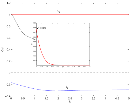
Figure 2: Graph of the best-possible bounds on qpis over $S_{k}$ for $k$ in the range $0$ to $5$. The inset graph, with $k$ in the range $0$ to $0.2$, shows that the upper bound lies above $1$, but converges rapidly to $1$ as $k$ increases.

IV..1 THE INFINITE WEDGE

An interesting subclass of hyperbolic regions is provided by taking the limit as $k\rightarrow 0$. The region $S_{0}$ so obtained is precisely the positive $(q,p)$ quadrant of $\Gamma$, as depicted in part (b) of Figure 1. Note that when $k=0$, the functions $d$ and $a$ take a simplified form:

$$d(\omega,0))\,=\,\tfrac{1}{2}\tanh(\pi\omega)\,,\quad a(\omega,0)\,=\,-\tfrac{1}{2}\tanh(\pi\omega)+u(\omega)\,,$$ (24)

where $u(\omega)$ may be expressed as an infinite sum ²⁸:

$$u(\omega)\,=\,\frac{8\omega}{\pi}\sum_{n=0}^{\infty}\frac{1}{\omega^{2}+(4n+1)^{2}}\,.$$

If we now apply these simplifications to the spectral formula (23), we obtain the spectrum for $\hat{\chi}_{0}$:

$$\mu_{\pm}(\omega,0)\,=\,\tfrac{1}{4}\left(1+\tanh(\pi\omega)\pm\sqrt{(2u(\omega)-\tanh(\pi\omega))^{2}+(1+\tanh(\pi\omega))^{2}}\right)\,,$$ (25)

which is graphed in Figure 3. The infimum and supremum can then be determined numerically, and to an accuracy of $\pm 5\times 10^{-10}$, we have that

$$-0.155939843\,<\,Q_{0}[W]\,<\,1.007679970.$$ (26)

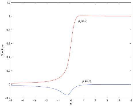
Figure 3: Graph of the spectrum of $\hat{\chi}_{0}$ which, as labeled, splits into the curves $\mu_{+}(\omega,0)$ and $\mu_{-}(\omega,0)$

An interesting point is that these bounds are also best-possible when applied to regions defined by infinite wedges. This equivalence is due to two factors: firstly, by an appropriate metaplectic transformation $T$, the region $S_{0}$ can be transformed into any infinite wedge with half-angle $\alpha<\pi/2$. Secondly, the operator transformation $\hat{U}_{T}$ that corresponds to $T$ is unitary, and thus the spectrum of $\hat{\chi}_{0}$ is preserved under its action. This implies that the spectrum of any region operator corresponding to an infinite wedge is given by (25). As a consequence, the integral of a Wigner function over any infinite wedge must lie between the bounds given in (26). Bounds on the spectrum of similar operators have been considered before, in the context of the quantum phase operator ²¹ and in connection with studies of probability backflow ²⁹ but not to the same level of precision.

V. EXAMPLES INVOLVING TWO BOUNDARY CURVES

As a second example, consider the slightly more complicated case of a region with a boundary composed of two curves with $T_{\sigma}$ symmetry. There are several possible forms that such a region can take ²⁷, however, we will concentrate on just the subcase for which the boundary curves lie in positive and negative $(q,p)$ quadrants, as shown in part (a) of Figure 4.

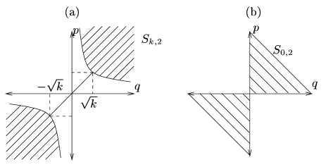
Figure 4: Regions bounded by two hyperbolic curves: in (a), the hyperbolic region $S_{k,2}$ is shown while in (b) the double wedge $S_{0,2}$ is depicted.

In order to further simplify matters, we assume that both curves are labeled by the variable $k$. We label the class of regions that remain by $S_{k,2}$ and note that this region may be written in terms of the region $S_{k}$ as

$$S_{k,2}\,=\,S_{k}+R_{\pi}(S_{k})\,,$$ (27)

where $R_{\pi}$ denotes a rotation through an angle $\pi$. Note that $R_{\pi}:(q,p)\rightarrow(-q,-p)$ and that the operator that corresponds to this transformation under the Weyl-Wigner transform is just the parity operator $\hat{P}$, which acts on the canonical coordinate and momentum operators according to

$$\hat{P}\hat{q}\hat{P}\,=\,-\hat{q}\,,\quad\hat{P}\hat{p}\hat{P}\,=\,-\hat{p}\,.$$

Due to the linearity of the Weyl quantization map, this implies that the region operator that corresponds to $S_{k,2}$ may be expressed as

$$\hat{\chi}_{k,2}\,=\,\hat{\chi}_{k}+\hat{P}\hat{\chi}_{k}\hat{P}\,.$$ (28)

This operator also commutes with $\hat{\omega}$, and hence its eigenstates can be chosen such that they are some linear combination of $\psi_{\omega}^{\pm}$. In order to find the correct linear combination, we must first determine the matrix representation of $\hat{\chi}_{k,2}$ on the subspace spanned by $\psi^{\pm}_{\omega}$. This turns out to quite simple, since the action of $\hat{P}$ on this subspace is given by $\hat{P}\psi_{\omega}^{\pm}=\psi_{\omega}^{\mp}$. Thus the matrix representation of $\hat{\chi}_{k,2}$ is given by

$$A_{2}(\omega,k)\,=\,A(\omega,k)+\left(\begin{array}[]{cc}0&1\\ 1&0\end{array}\right)A(\omega,k)\left(\begin{array}[]{cc}0&1\\ 1&0\end{array}\right)\,=\,\left(\begin{array}[]{cc}\tfrac{1}{2}+d(\omega,k)&a(\omega,k)\\ a(\omega,k)&\tfrac{1}{2}+d(\omega,k)\end{array}\right)\,.$$ (29)

The simple form of this matrix representation leads to the following expression for the spectrum of $\hat{\chi}_{k,2}$:

$$\mu_{2,\pm}(\omega,k)\,=\,\frac{1}{2}+d(\omega,k)\pm|a(\omega,k)|\,,$$ (30)

In this case, the eigenfunctions are odd and even combinations of $\psi_{\omega}^{\pm}$, and are independent of $k$:

$$\psi^{\pm}_{2,\omega}(x;k)\,\equiv\psi^{\pm}_{2,\omega}(x)\,=\,\frac{1}{\sqrt{2}}\left(\psi_{\omega}^{+}(x)\pm\psi_{\omega}^{-}(x)\right)\,,$$ (31)

which indicates that the operators $\hat{\chi}_{k,2}$ commute for all $k\geq 0$.

The properties of the spectrum in this case vary somewhat from the preceding example. In particular, $\mu_{2,-}(\omega,k)$ is not restricted to negative values and, similarly, $\mu_{2,+}(\omega,k)$ is not strictly positive, although clearly the inequality $\mu_{2,+}(\omega,k)\geq\mu_{2,-}(\omega,k)$ holds for all $\omega\in\mathbb{R},k\geq 0$. Since the bounds on qpis over $S_{k,2}$ are given by the infimum $L_{k,2}$ and supremum $U_{k,2}$ of the spectrum of $\hat{\chi}_{k,2}$, it is these functions that are of primary importance in the context of this paper. Again, closed-form expressions do not appear to exist, so we must resort to computational techniques in evaluating these functions, the results of which are graphed in Figure 5. In this case, the upper bound is well in excess of $1$ for small values of $k$, but rapidly approaches $1$ as $k$ increases. The lower bound, on the other hand, dips initially, reaching a minimum of $-0.4014$ at $k=0.4$ before rising again, and appears to approach a finite negative value near to $-0.3$ as $k\rightarrow\infty$.

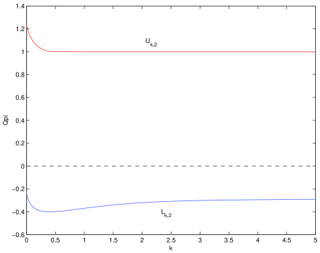
Figure 5: Graph of the best-possible bounds on qpis over $S_{k,2}$ for $k$ in the range $0$ to $5$.

V..1 DOUBLE WEDGES

It is again of interest to consider in more detail the limit as $k\rightarrow 0$ of the region $S_{k,2}$. The resulting region $S_{0,2}$ is the union of the positive and negative $(q,p)$ quadrants (as shown in part (b) of Figure 4, and one might guess that qpis over such a region should be positive ²⁴, since it appears to composed from the union of a set of infinite straight lines, over which the integral of the Wigner function is known to be positive. However, since these lines cross at the origin one cannot immediately apply this result and it will be shown that the true bounds on qpis lie significantly outside the $[0,1]$ interval to which classical probabilities are restricted.

The region operator that corresponds to $\hat{\chi}_{0,2}$ may be expressed in terms of $\hat{\chi}_{0}$ as $\hat{\chi}_{0,2}=\hat{\chi}_{0}+\hat{P}\hat{\chi}_{0}\hat{P}$. The spectrum for this operator can be derived from (30) upon substitution of (24), from which we obtain

$$\mu_{2,\pm}(\omega,0)\,=\,\frac{1+\tanh(\pi\omega)}{2}\pm\left|u(\omega)-\frac{\tanh(\pi\omega)}{2}\right|\,.$$ (32)

This spectrum is graphed in Figure 6, and from this one sees that the function $\mu_{2}=\tfrac{1}{2}+u(\omega)$ passes through both the infimum and the supremum of the spectrum of $\hat{\chi}_{0,2}$. Since $u(\omega)$ is an odd function, we need only calculate its global maximum in order to determine the bounds on qpis over $S_{0,2}$. Using computational techniques, this value can be obtained to great accuracy, and we find that the best-possible bounds (accurate to $\pm 5\times 10^{-10}$) on qpis over $S_{0,2}$ are

$$-0.236823652\,<\,Q_{\alpha,2}[W]\,<\,1.236823652\,.$$ (33)

Note that the upper and lower bounds sum to $1$ since they are symmetric about $1/2$. This symmetry can be explained by noting that if one rotates the region $S_{0,2}$ through an angle $\pi/2$, then one obtains its complement: i.e. $R_{\pi/2}(S_{0,2})=\Gamma/S_{0,2}=S_{0,2}^{c}$. Note that the integral of a Wigner function over $\Gamma=S\cup S^{c}$ is normalized to $1$. Now, since the operator equivalent of a rotation is a unitary transformation, the region operator that corresponds to the complement of $S_{0,2}$ has precisely the spectrum given in (32). Accordingly, the spectrum of $\hat{\chi}_{0,2}$ must consist of pairs that sum to $1$ and, in particular, the upper and lower bounds on this spectrum must be symmetric about $1/2$.

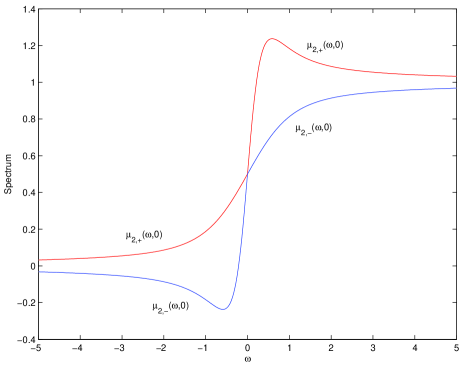
Figure 6: Spectrum of the double wedge operator $\hat{\chi}_{0,2}$.

As in the case of the region $S_{0}$, the bounds on qpis over $S_{0,2}$ can be applied to a wider class of regions. We shall refer to elements of this wider class as double wedges, since they are formed by taking the union of an infinite wedge with its rotation through an angle $\pi$. By applying the appropriate metaplectic transformation, we can transform $S_{0,2}$ into any double wedge. The corresponding operator transformation is unitary and preserves the spectrum of $\hat{\chi}_{0,2}$, so that the spectrum of any region operator corresponding to a double wedge is given by (32). Accordingly, the integral of any Wigner function over an arbitrary double wedge must satisfy the inequality given in (33).

VI. CONCLUSION

The problem of constructing best possible bounds on integrals of the Wigner function is not only of mathematical interest, but should be of practical significance in providing checks on experimentally reconstructed quantum states. Since our approach to the problem relies on specifying the region to be integrated over, it is important to identify the types of region for which the bounds can be easily computed. In this paper, we have considered several examples of regions with a hyperbolic symmetry for which the bounds can be computed numerically from the spectrum of an exactly solvable integral equation. We have demonstrated that the bounds on integrals of the Wigner function for these regions are not equivalent to those on integrals of true probability density functions. In particular, the lower bound is significantly below zero in all cases, although it lacks the scalloped effect arising from eigenvalue crossings as seen in the bounds for elliptical discs ¹⁷. The upper bound also rises above $1$ although for the most part the difference between its value and the classical bound is very small. This contrasts with the case of the disc, for which the upper bound always remains below $1$.

Figure 7: Examples of generalized hyperbolic regions are shown in (a)-(c).

The results herein can also be extended to more complicated regions with boundaries given by an arbitrary number of hyperbolic curves sharing the same symmetry ²⁷, for example, the regions shown in Figure 7. The problem of determining the spectrum is essential the same but the matrix representations for operators corresponding to regions with many boundaries are functions of many variables and hence the behaviour of the bounds is much more difficult to characterize.

APPENDIX

The configuration kernels that correspond to (13) take the form

$$\chi_{k,K}(x,y)\,=\,\frac{H(\tfrac{x+y}{2})}{2\pi}\int_{-\infty}^{\infty}H(p-\tfrac{2k}{x+y})e^{i(x-y)p}dp\,.$$ (A-1)

This integral can be computed in a generalized sense ³⁰, and we find that

$$\chi_{k,K}(x,y)\,=\,H(\tfrac{x+y}{2})e^{2ik\frac{x-y}{x+y}}\left[\tfrac{1}{2}\delta(x-y)-\frac{1}{2\pi i(x-y)}\right]\,.$$ (A-2)

This expression for the configuration kernel of $\hat{\chi}_{k}$ enables us to determine the action of $\hat{\chi}_{k}$ on the space $\mathcal{G}^{\prime}_{\omega}$ (recall that this is given by the matrix $A(\omega,k)$ defined in (19)) . In this representation $\hat{\chi}_{k}$ acts on $\psi_{\omega}$ as

$$(\hat{\chi}_{k}\psi_{\omega})(x)\,=\,\int_{-x}^{\infty}e^{2ik\frac{x-y}{x+y}}\left[\tfrac{1}{2}\delta(x-y)-\frac{1}{2\pi i(x-y)}\right]\psi_{\omega}(y)dy\,.$$ (A-3)

If we substitute $\psi_{\omega}=\alpha_{\omega}\psi_{\omega}^{+}+\beta_{\omega}\psi_{\omega}^{-}$, then we find that the action of $\hat{\chi}_{k}$ when $x<0$ differs from that when $x>0$. Thus, for $x>0$,

$$(\hat{\chi}_{k}\psi_{\omega})(x) = \alpha_{\omega}\int_{0}^{\infty}e^{2ik\frac{x-y}{x+y}}\left[\tfrac{1}{2}\delta(x-y)-\frac{1}{2\pi i(x-y)}\right]\frac{e^{i\omega\log y}}{\sqrt{2\pi y}}dy$$

$$+ \beta_{\omega}\int_{-x}^{0}e^{2ik\frac{x-y}{x+y}}\left[\tfrac{1}{2}\delta(x-y)-\frac{1}{2\pi i(x-y)}\right]\frac{e^{i\omega\log|y|}}{\sqrt{2\pi|y|}}dy$$

and for $x<0$,

$$(\hat{\chi}_{k}\psi_{\omega})(x)\,=\,\alpha_{\omega}\int_{|x|}^{\infty}e^{2ik\frac{x-y}{x+y}}\left[\tfrac{1}{2}\delta(x-y)-\frac{1}{2\pi i(x-y)}\right]\frac{e^{i\omega\log y}}{\sqrt{2\pi y}}dy\,.$$

It is immediately clear that $A_{22}(\omega,k)=0$, since the $x>0$ case involves only $\alpha_{\omega}$.

The other integrals can be simplified and this process leads to the following expression for the matrix elements of $A$:

$$A(\omega,k)\,=\,\left(\begin{array}[]{cc}\tfrac{1}{2}+d(\omega,k)&\tfrac{1}{2}[a(\omega,k)+ib(\omega,k)]\\ \tfrac{1}{2}[a(\omega,k)-ib(\omega,k)]&0\end{array}\right)\,,$$ (A-4)

where the functions $d,a$ and $b$ are given by

$$d(\omega,k) = \frac{1}{2\pi}\int_{0}^{\infty}\frac{\sin(\omega t-2k\tanh(t/2))}{\sinh(t/2)}dt\,,$$ (A-5)

$$a(\omega,k) = \frac{1}{2\pi}\int_{0}^{\infty}\frac{\sin(\omega t-2k\coth(t/2))}{\cosh(t/2)}dt\,,$$ (A-6)

$$b(\omega,k) = \frac{1}{2\pi}\int_{0}^{\infty}\frac{\cos(\omega t-2k\coth(t/2))}{\cosh(t/2)}dt.$$ (A-7)

Note, however, that although the integrands of $a$ and $b$ are bounded for all $t$, they become highly oscillatory in the neighbourhood of the origin, which poses difficulties for numerical schemes. These problems can be alleviated by using the technique of contour integration.

In the case of $b(\omega,k)$, we consider the following contour integral in the complex plane

$$I_{C}=\frac{1}{2\pi}\oint_{C}\frac{e^{i\omega z-2ik\coth(z/2)}}{\cosh(z/2)}dz\,,$$ (A-8)

where $C$ is the contour shown in part (a) of Figure 8. Although the contour is divided into four parts, only the integrals along the real axis contribute, since the contributions from the semi-circular segments vanish in the respective limits as $\epsilon\rightarrow 0$ and $R\rightarrow\infty$. Thus one has that

$$\lim_{R\rightarrow\infty,\epsilon\rightarrow 0}I_{C}\,=\,2\frac{1}{2\pi}\int_{0}^{\infty}\frac{e^{i\omega t-2ik\coth(t/2)}}{\cosh(t/2)}dt\,,$$ (A-9)

and as a result, $b(\omega,k)\,=\,\Re\{I_{C}\}/2$.

Figure 8: The contours used in evaluating the functions $b(\omega,k),a(\omega,k)$ and $d(\omega,k)$: in (a), the semi-circular contour $C$, in (b), the contour $C^{\prime}$ used to relate $b(\omega,k)$ to $d(\omega,k)$ and in (c), an example of a contour $C_{0}$ for evaluating $R(\omega,k)$.

We can make use of the residue theorem in evaluating $I_{C}$:

$$I_{C}\,=\,2\pi i\sum\textrm{Res}f(z)\,,$$ (A-10)

where $f(z)$ is the integrand in (A-8). Note that $f(z)$ has two distinct classes of residues: simple poles at $z=(2n+1)\pi i$ and essential singularities at $z=2m\pi i$, with $m\in\mathbb{Z}$. The contour $C$ encloses only the simple poles with $n\geq 0$ and the essential singularities with $m\geq 1$, and hence the sum in (A-10) is over the residues at these points.

It is easy to evaluate the residues at the simple poles and we find that the total contribution from the simple poles inside $C$ is given by

$$\textrm{Res}_{s}\,=\,\frac{1}{2\pi i}\sum_{n=0}^{\infty}(-1)^{n}e^{-(2n+1)\pi\omega}\,=\,\frac{\textrm{sech}(\pi\omega)}{2\pi i}\,.$$ (A-11)

The sum of the residues associated with the essential singularities can also be simplified:

$$\textrm{Res}_{e}\,=\,\frac{1}{2\pi}\sum_{n=1}^{\infty}(-1)^{n}e^{-2n\pi\omega}R(\omega,k)\,=\,=\frac{e^{-\pi\omega}\textrm{sech}(\pi\omega)}{2}R(\omega,k)\,,$$ (A-12)

where $R(\omega,k)$ is the residue of $f(z)$ associated with the essential singularity at the origin.

Ordinarily, one might try to evaluate this residue by constructing the Laurent series for $f(z)$, however in this case the $\coth$ term in the exponential makes this extremely difficult. However, one may use the residue theorem in reverse and evaluate $R(\omega,k)$ by considering the integral of $f(z)$ over a closed contour enclosing the origin (and no other poles):

$$R(\omega,k)\,=\,\frac{1}{2\pi i}\oint_{C_{1}}\frac{e^{i\omega z-2ik\coth(z/2)}}{\cosh(z/2)}dz\,.$$ (A-13)

The rapid oscillations due to the $\coth$ term do not appear in this calculation, and due to its finite range this integral can be rapidly evaluated to a high degree of accuracy using numerical techniques.

If we now collect the results for the residues together, we discover that

$$b(\omega,k)\,=\,\frac{\textrm{sech}(\pi\omega)}{2}\left[1+\frac{e^{-\pi\omega}}{2}\Im\{R(\omega,k)\}\right]\,.$$ (A-14)

Note that in deriving these results it has been assumed that $\omega\geq 0$. A similar procedure (with the semi-circular contour defined in the lower half plane) enables us to extend the validity of (A-14) to all $\omega\in\mathbb{R}$.

In order to obtain superior expressions for the functions $a(\omega,k)$ and $d(\omega,k)$, we choose another contour (see part (b) of Figure 8), this time involving five curves. However, we know from the above calculation that the integral over $\epsilon_{0}$ vanishes, which leaves four curves to consider. Of these, the integral over the imaginary axis from $0$ to $\pi$ results in a pure imaginary contribution $I_{\pi}$, while the integral over $\epsilon_{1}$ contributes $-1/2$ in the limit as $\epsilon_{1}\rightarrow 0$. The integral over the positive real axis is equal to $b(\omega,k)+a(\omega,k)i$ in the limit as $\epsilon_{0}\rightarrow 0$, while the contribution from the line $(\pi i,\pi i+\infty)$ can be expressed as $-\exp(-\pi\omega)(d(\omega,k)+I_{\infty}i)$.

By equating the real parts, we find that

$$b(\omega,k)\,=\,e^{-\pi\omega}(\tfrac{1}{2}+d(\omega,k))\,.$$ (A-15)

This leads to the expression (20) for $d(\omega,k)$ and the expression (22) for the matrix $A$. If we equate the imaginary parts, then we discover that

$$a(\omega,k)\,=\,e^{-\pi\omega}(I_{\pi}-I_{\infty})\,,$$ (A-16)

where

$$I_{\pi} = \frac{1}{2\pi}\int_{0}^{\pi}\frac{e^{\omega t-2ktan(t/2)}}{\sin(t/2)}dt\,,$$ (A-17)

$$I_{\infty} = \frac{1}{2\pi}\int_{0}^{\infty}\frac{\cos(\omega t-2k\tanh(t/2))}{\sinh(t/2)}dt\,.$$ (A-18)

Neither $I_{\pi}$ nor $I_{\infty}$ are well-defined, but their difference is, and provided one expresses $a(\omega,k)$ as in (21), the singularities of these integrals are avoided.

References

- 1 E. P. Wigner, Phys. Rev., 40, 749 (1932).
- 2 H. Groenewold, Physica, 12, 405 (1946).
- 3 J. Moyal, Proc. Camb. Phil. Soc., 45, 99 (1949).
- 4 M. Hillery, R. F. O’Connell, M. O. Scully and E. P. Wigner, Phys. Rep., 106, 121 (1984).
- 5 W. P. Schleich, Quantum Optics in Phase Space, (Wiley-VCH, Weinheim, 2001).
- 6 H. Mori, I. Oppenheim and J. Ross in Studies in Statistical Mechanics, edited by J. de Boer and G. E. Uhlenbeck (North Holland, Amsterdam, 1962) Vol. 1, pp. 213–298.
- 7 P. Carruthers and F. Zachariasen, Rev. Modern Phys. 55, 245 (1983).
- 8 L. Cohen, Proc. IEEE, 77, 941 (1989).
- 9 L. Cohen, Time-Frequency Analysis, (Prentice Hall, New Jersey, 1995).
- 10 W. Williams, Proc. IEEE, 84, 1264 (1996).
- 11 M. Raymer, Contemp. Phys., 38, 343 (1997).
- 12 G. A. Baker Jr., Phys. Rev., 109, 2198 (1958).
- 13 R. Price and E. Hofstetter, IEEE Trans. Inf. Theory, 11, 207 (1965).
- 14 N. G. de Bruijn, in Inequalities, edited by O. Shisha (Academic Press, New York, 1967), pp. 57–71.
- 15 A. J. E. M. Janssen, Rep. Math. Phys., 6, 249 (1974).
- 16 E. H. Lieb, J. Math. Phys., 31, 594 (1990).
- 17 A. J. Bracken, H.-D. Doebner and J. G. Wood, Phys. Rev. Lett., 83, 3758 (1999).
- 18 A. J. Bracken, D. E. Ellinas and J. G. Wood, In Proceedings of the Wigner Centennial Conference, Pecs, Hungary, 2002, pages 63 1-4, http://quantum.ttk.pte.hu/wigner/proceedings/papers/w63.pdf.
- 19 A. J. Bracken, D. E. Ellinas and J. G. Wood, J. Phys. A, 36, L297 (2003).
- 20 H. Weyl, The theory of groups and quantum mechanics, (Dover, New York, 1931) p274.
- 21 D. A. Dubin, M. A. Hennings and T. B. Smith, Mathematical Aspects of Weyl Quantization and Phase. (World Scientific, Singapore, 2000) pp263-268.
- 22 T. Osborn and F. Molzahn, Ann. Phys., 241, 79 (1995).
- 23 A. J. Bracken, G. Cassinelli and J. G. Wood, J. Phys. A, 36, 1033 (2003).
- 24 J. Bertrand and P. Bertrand, Found. Phys., 17, 397 (1987).
- 25 D. Chruscinski, J. Math. Phys., 44, 3718 (2003).
- 26 I. M. Gel’fand, Generalized functions, (Academic Press, New York, 1964-68).
- 27 J. G. Wood, PhD. Thesis, (Department of Mathematics, University of Queensland, 2004).
- 28 I. S. Gradshteyn and I. M. Ryzhik, Tables of Integrals, Series and Products, 6th Edition, (Academic Press, San Diego, 2000).
- 29 A. J. Bracken and G. F. Melloy, J. Phys. A, 27, 2197 (1994).
- 30 I. N. Sneddon, Fourier Transforms, (McGraw Hill, New York, 1951).