Qubiter Algorithm Modification, Expressing Unstructured Unitary Matrices
with Fewer CNOTs

Abstract

A quantum compiler is a software program for decomposing (“compiling”) an arbitrary unitary matrix into a sequence of elementary operations (SEO). The author of this paper is also the author of a quantum compiler called Qubiter. Qubiter uses a matrix decomposition called the Cosine-Sine Decomposition (CSD) that is well known in the field of Computational Linear Algebra. One way of measuring the efficiency of a quantum compiler is to measure the number of CNOTs it uses to express an unstructured unitary matrix (a unitary matrix with no special symmetries). We will henceforth refer to this number as $\epsilon$. In this paper, we show how to improve $\epsilon$ for Qubiter so that it matches the current world record for $\epsilon$, which is held by another quantum compiling algorithm based on CSD.

1 Introduction

In quantum computing, elementary operations are operations that act on only a few (usually one or two) qubits. For example, CNOTs and one-qubit rotations are elementary operations. A quantum compiling algorithm is an algorithm for decomposing (“compiling”) an arbitrary unitary matrix into a sequence of elementary operations (SEO). A quantum compiler is a software program that implements a quantum compiling algorithm.

Henceforth, we will refer to Ref.[1] as Tuc99. Tuc99 gives a quantum compiling algorithm, implemented in a software program called Qubiter. The Tuc99 algorithm uses a matrix decomposition called the Cosine-Sine Decomposition (CSD) that is well known in the field of Computational Linear Algebra. Tuc99 uses CSD in a recursive manner. It decomposes any unitary matrix into a sequence of diagonal unitary matrices and something called uniformly controlled U(2) gates. Tuc99 then expresses these diagonal unitary matrices and uniformly controlled U(2) gates as SEOs of short length.

More recently, two other groups have proposed quantum compiling algorithms based on CSD. One group, based at the Univ. of Michigan and NIST, has published Ref.[2], henceforth referred to as Mich04. Another group based at Helsinki Univ. of Tech.(HUT), has published Refs.[3]. and [4], henceforth referred to as HUT04a and HUT04b, respectively.

One way of measuring the efficiency of a quantum compiler is to measure the number of CNOTs it uses to express an unstructured unitary matrix (a unitary matrix with no special symmetries). We will henceforth refer to this number as $\epsilon$. Although good quantum compilers will also require optimizations that deal with structured matrices, unstructured matrices are certainly an important case worthy of attention. Minimizing the number of CNOTs is a reasonable goal, since a CNOT operation (or any 2-qubit interaction used as a CNOT surrogate) is expected to take more time to perform and to introduce more environmental noise into the quantum computer than a one-qubit rotation. Ref.[5] proved that for unitary matrices of dimension $2^{N_{B}}$ (${N_{B}}=$ number of bits), $\epsilon\geq\frac{1}{4}(4^{N_{B}}-3{N_{B}}-1)$. This lower bound is achieved for ${N_{B}}=2$ by the 3 CNOT circuits first proposed in Ref.[6]. It is not known whether this bound can always be achieved for ${N_{B}}>3$.

The Mich04 and HUT04b algorithms try to minimize $\epsilon$. In this paper, we propose a modification of the Tuc99 algorithm which will henceforth be referred to as Tuc04. Tuc04 comes in two flavors, Tuc04(NR) without relaxation process, and Tuc04(R) with relaxation process. As the next table shows, the most efficient algorithm known at present is Mich04. HUT04b performs worse than Mich04. Tuc04(R) and Mich04 are equally efficient.

algorithm	$\epsilon$
Tuc99	$O(2^{2{N_{B}}})$
Mich04	$2^{2{N_{B}}-1}-3(2^{{N_{B}}-1})+1=(2^{N_{B}}-1)(2^{{N_{B}}-1}-1)$
HUT04b	$2^{2{N_{B}}-1}-(2^{{N_{B}}-1})-2=(2^{N_{B}}-1)(2^{{N_{B}}-1}-1)+2^{N_{B}}+O(1)$
Tuc04(NR)	$(2^{N_{B}}-1)(2^{{N_{B}}-1}-1)+2^{N_{B}}$
Tuc04(R)	$(2^{N_{B}}-1)(2^{{N_{B}}-1}-1)$

Caveat: Strictly speaking, the efficiency of Tuc04(R) as listed in this table is only a conjecture. The problem is that Tuc04(R) uses a relaxation process. This paper argues, based on intuition, that the relaxation process converges, but it does not prove this rigorously. A rigorous proof of the efficiency of Tuc04(R) will require theoretical and numerical proof that its relaxation process converges as expected.

2 Notation

This paper is based heavily on Tuc99 and assumes that the reader is familiar with the main ideas of Tuc99. Furthermore, this paper uses the notational conventions of Tuc99. So if the reader can’t follow the notation of this paper, he/she is advised to consult Tuc99. The section on notation in Ref. [7] is also recommended.

Contrary to Tuc99, in this paper we will normalize Hadamard matrices so that their square equals one.

As in Tuc99, for a single qubit with number operator $n$, we define $P_{0}=n$ and $P_{1}=\overline{n}=1-n$. If $\vec{\kappa}=(\kappa_{1},\kappa_{2},\ldots,\kappa_{N_{K}})$ labels ${N_{K}}$ distinct qubits and $\vec{b}=(b_{1},b_{2},\ldots,b_{{N_{K}}})\in Bool^{N_{K}}$, then we define $P_{{\vec{b}}}(\vec{\kappa})=P_{b_{1}}(\kappa_{1})P_{b_{2}}(\kappa_{2})\ldots P_{b_{N_{K}}}(\kappa_{N_{K}})$.

When we say $A$ (ditto, $A^{\prime}$) is $B$ (ditto, $B^{\prime}$), we mean $A$ is $B$ and $A^{\prime}$ is $B^{\prime}$.

For any complex number $z$, we will write $z=|z|e^{i\angle(z)}$. Thus, $|z|$ and $\angle(z)$ are the magnitude and phase angle of $z$, respectively.

${\hat{e}}_{x},{\hat{e}}_{y},{\hat{e}}_{z}$ will denote the unit vectors along the X, Y, Z axes, respectively. For any 3d real unit vector ${\hat{s}}$, $\sigma_{s}=\vec{\sigma}\cdot{\hat{s}}$, where $\vec{\sigma}=({\sigma_{x}},{\sigma_{y}},{\sigma_{z}})$ is the vector of Pauli matrices.

3 $U(N)$-subsets and $U(N)$-Multiplexors

We define a $U(N)$-subset to be an ordered set $\{U_{b}\}_{\forall b}$ of $N$ dimensional unitary matrices. Let the index $b$ take values in a set $S_{\underline{b}}$ with $N_{\underline{b}}$ elements. In this paper, we are mostly concerned with the case that $S_{\underline{b}}=Bool^{{N_{K}}}$, and $b$ is represented by $\vec{b}$.

Suppose a qubit array with ${N_{B}}$ qubits is partitioned into ${N_{T}}$ target qubits and ${N_{K}}$ control qubits. Thus, ${N_{T}},{N_{K}}$ are positive integers such that ${N_{B}}={N_{T}}+{N_{K}}$. Let $\vec{\kappa}=(\kappa_{1},\kappa_{2},\ldots,\kappa_{N_{K}})$ denote the control qubits and $\vec{\tau}=(\tau_{1},\tau_{2},\ldots,\tau_{N_{T}})$ the target qubits. Thus, if $\vec{\tau}$ and $\vec{\kappa}$ are considered as sets, they are disjoint and their union is $\{0,1,\ldots,{N_{B}}-1\}$. Let $\{U_{\vec{b}}\}_{\forall{\vec{b}}\in Bool^{N_{K}}}$ be an ordered set of operators all of which act on the Hilbert space of the target qubits. We will refer to any operator $X$ of the following form as a uniformly controlled $U(2^{N_{T}})$-subset, or, more succinctly, as a $U(2^{N_{T}})$-multiplexor:

$$X=\sum_{{\vec{b}}\in Bool^{N_{K}}}P_{{\vec{b}}}(\vec{\kappa})U_{\vec{b}}(\vec{\tau})=\prod_{{\vec{b}}\in Bool^{N_{K}}}U_{\vec{b}}(\vec{\tau})^{P_{{\vec{b}}}(\vec{\kappa})}\;.$$ (1)

(“multiplexor” means “multi-fold” in Latin. A special type of electronic device is commonly called a multiplexor or multiplexer). Note that $X$ is a function of: a set $\vec{\kappa}$ of control bits, a set $\vec{\tau}$ of target bits, and a $U(2^{N_{T}})$-subset $\{U_{\vec{b}}\}_{\forall{\vec{b}}\in Bool^{N_{K}}}$. Fig.1 shows two possible diagrammatic representations of a multiplexor, one more explicit than the other. The diagrammatic representation with the “half moon” nodes was introduced in Ref.[3].

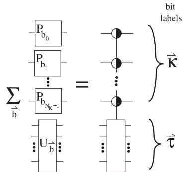
Figure 1: 2 Diagrammatic representations of a $U(2^{N_{T}})$-multiplexor.

For a given $U(2)$-subset $\{U_{b}\}_{\forall b}$ (and for any multiplexor with that $U(2)$-subset), it is useful to define as follows what we shall call the optimal axis of the $U(2)$-subset. Suppose that we express each $U_{b}$ in the form

$$U_{b}=e^{i\eta_{b}}e^{i{\sigma_{z}}\gamma_{b}}e^{i({\sigma_{s_{1}}}\alpha_{b}+{\sigma_{s_{2}}}\beta_{b})}(i{\sigma_{w}})^{f(b)}\;,$$ (2)

where $\eta_{b},\alpha_{b},\beta_{b},\gamma_{b}$ are real parameters, where the vectors ${\hat{s}}_{1},{\hat{s}}_{2}$, and ${\hat{w}}={\hat{s}}_{1}\times{\hat{s}}_{2}$ are orthonormal, and where $f(b)$ is an indicator function which maps the set of all possible $b$ into $\{0,1\}$. Of course, $e^{i\eta_{b}}=\sqrt{\det{U_{b}}}$. Appendix A shows how to find the parameters $\alpha_{b},\beta_{b},\gamma_{b}$ for a given $U_{b}e^{-i\eta_{b}}\in SU(2)$. Appendix B solves the following minimization problem. If the value of the parameters $\alpha_{b},\beta_{b},\gamma_{b}$ and the vectors ${\hat{s}}_{1},{\hat{s}}_{2},{\hat{w}}$ are allowed to vary, while keeping the vectors ${\hat{s}}_{1},{\hat{s}}_{2},{\hat{w}}$ orthonormal and keeping all $U_{b}$ fixed, find vectors ${\hat{s}}_{1},{\hat{s}}_{2},{\hat{w}}$ that are optimal, in the sense that they minimize a cost function. The cost function penalizes deviations of the diagonal matrices $e^{i\gamma_{b}{\sigma_{z}}}$ away from the 2d identity matrix $I_{2}$. Any choice of orthonormal vectors ${\hat{s}}_{1},{\hat{s}}_{2}$ will be called strong directions and ${\hat{w}}={\hat{s}}_{1}\times{\hat{s}}_{2}$ will be called a weak direction, or an axis of the $U(2)$-subset. An axis that minimizes the cost function will be called the optimum axis of the $U(2)$-subset. (an axis of goodness).

It is also possible to define an optimum axis of a $U(2)$-subset in the same way as just discussed, except replacing Eq.(2) by

$$U_{b}=e^{i\eta_{b}}(i{\sigma_{w}})^{f(b)}e^{i({\sigma_{s_{1}}}\alpha_{b}+{\sigma_{s_{2}}}\beta_{b})}e^{i{\sigma_{z}}\gamma_{b}}\;.$$ (3)

In Eq.(2), the diagonal matrix $e^{i\gamma{\sigma_{z}}}$ is on the left hand side, so we will call this the diagonal-on-left (DOL) parameterization. In Eq.(3), the diagonal matrix $e^{i\gamma{\sigma_{z}}}$ is on the right hand side, and we will call this the diagonal-on-right (DOR) parameterization.

4 Tuc04 algorithm

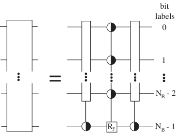
Figure 2: Diagrammatic representation of the Cosine-Sine Decomposition (CSD).

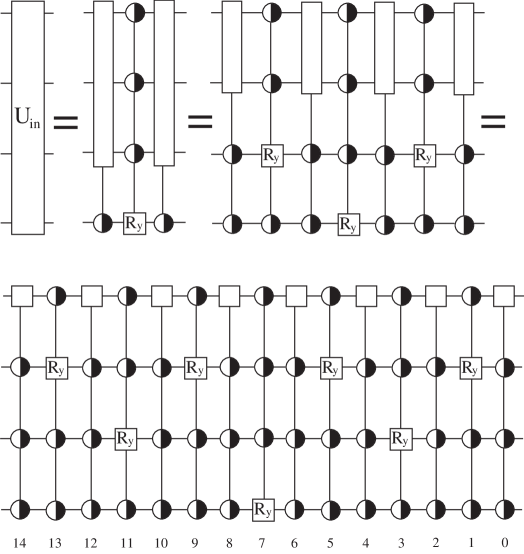
Figure 3: Recursive use of CSD to decompose a $2^{4}$ dimensional unitary matrix.

The Cosine Sine Decomposition (CSD) expresses an $N$ dimensional unitary matrix $U$ as a product $LDR$, where $L=L_{0}\oplus L_{1}$, $D=e^{i{\sigma_{y}}\otimes\Theta}$, $R=R_{0}\oplus R_{1}$, where $L_{0},L_{1},R_{0},R_{1}$ are unitary matrices of dimension $N/2$, and $\Theta$ is a diagonal real matrix whose entries can be interpreted as angles between subspaces. Note that the matrices $L,D$ and $R$ are all multiplexors. Fig.2 depicts the CSD graphically, using the multiplexor symbol of Fig.1. In Fig.2, a $U(2)$-multiplexor whose $U(2)$-subset consists solely of rotations around the Y axis, is indicated by putting the symbol $R_{y}$ in its target box. We will call this type of multiplexor an $R_{y}(2)$-multiplexor.

Lets review the Tuc99 algorithm. It decomposes an arbitrary unitary matrix into a SEO by applying the CSD in a recursive manner. The beginning of the Tuc99 algorithm for ${N_{B}}=4$ is illustrated in Fig.3. An initial unitary matrix $U_{in}$ is decomposed via CSD into a product of 3 multiplexors $L,D,R$. The $L$ and $R$ multiplexors on each side of $D$ are in turn decomposed via CSD. The $L$ and $R$ multiplexors generated via any application of CSD are in turn decomposed via CSD. In Fig.3, we have stopped recursing once we reached multiplexors whose target box acts on a single qubit. Note that at this stage, $U_{in}$ is decomposed into a product of $U(2)$-multiplexors. There are $1+2+4+\ldots+2^{{N_{B}}-1}=2^{{N_{B}}}-1$ of these $U(2)$-multiplexors (15 for ${N_{B}}=4$). Half of these $U(2)$-multiplexors have $R_{y}$ in their target boxes and the other half don’t. Furthermore the $R_{y}$ type multiplexors and non-$R_{y}$ ones alternate. Furthermore, the non-$R_{y}$ $U(2)$-multiplexors have their target box at qubit 0, so, according to the conventions of Tuc99, they are direct sums of $U(2)$ matrices. The Tuc99 algorithm deals with these direct sums of $U(2)$ matrices by applying CSD to each $U(2)$ matrix in the direct sum. This converts each direct sum of $U(2)$ matrices into a product $LDR$, where $R$ and $L$ are diagonal unitary matrices and $D$ is an $R_{y}(2)$-multiplexor. Thus, Tuc99 turns the last operator sequence shown in Fig.3 into a sequence of alternating diagonal unitary matrices and $R_{y}(2)$-multiplexors. Then Tuc99 gives a prescription for decomposing any diagonal unitary matrix into a SEO with $2^{{N_{B}}}$ CNOTs and any $R_{y}(2)$-multiplexor into a SEO with $2^{{N_{B}}-1}$ CNOTs.

Tuc99 considers what it calls a $D$-matrix:

$$D=\exp(\sum_{{\vec{b}}\in Bool^{{N_{B}}-1}}i\Phi_{\vec{b}}\otimes P_{\vec{b}})=\sum_{{\vec{b}}\in Bool^{{N_{B}}-1}}U_{\vec{b}}\otimes P_{\vec{b}}\;,$$ (4a)

with

$$U_{\vec{b}}=\exp(i\Phi_{\vec{b}})\;,$$ (4b)

where

$$\Phi_{\vec{b}}=\phi_{\vec{b}}{\sigma_{y}}\;.$$ (5)

Here $\phi_{\vec{b}}$ is a real parameter. In the nomenclature of this paper, $D$ is an $R_{y}(2)$-multiplexor with a single target qubit at ${N_{B}}-1$ and ${N_{B}}-1$ control qubits at $\{0,1,\ldots,{N_{B}}-2\}$. Tuc99 shows how to decompose $D$ into a SEO with $2^{{N_{B}}-1}$ CNOTs. Tuc99 also discusses how, by permuting qubits via the qubit exchange operator, one can move the target qubit to any position $\{0,1,\ldots,{N_{B}}-1\}$ to get what Tuc99 calls a direct sum of $D$ matrices. In the nomenclature of this paper, a “direct sum of $D$ matrices” is just an $R_{y}(2)$-multiplexor with a single target qubit at any position out of $\{0,1,\ldots,{N_{B}}-1\}$. In conclusion, Tuc99 gives a complete discussion of $R_{y}(2)$-multiplexors and how to decompose them into a SEO with $2^{{N_{B}}-1}$ CNOTs.

Next, let us consider how to generalize Tuc99. We begin by proving certain facts about $U(2)$-multiplexors that are generalizations of similar facts obtained in Tuc99 for $R_{y}(2)$-multiplexors.

Suppose ${\hat{s}}_{1},{\hat{s}}_{2}$ and ${\hat{w}}={\hat{s}}_{1}\times{\hat{s}}_{2}$ are orthonormal vectors. Suppose we generalize the $D$ matrices of Tuc99 by using Eqs.(4) with:

$$\Phi_{\vec{b}}=\phi_{{\vec{b}},1}{\sigma_{s_{1}}}+\phi_{{\vec{b}},2}{\sigma_{s_{2}}}\;.$$ (6)

Here $\phi_{{\vec{b}},x}$ and $\phi_{{\vec{b}},y}$ are real parameters. In Tuc99, we define $\vec{\phi}$ to be a column vector whose components are the numbers $\phi_{\vec{b}}$ lined up in order of increasing ${\vec{b}}\in Bool^{{N_{B}}-1}$. Here, we use the same rule to define vectors $\vec{\phi}_{x}$ and $\vec{\phi}_{y}$ from $\phi_{{\vec{b}},x}$ and $\phi_{{\vec{b}},y}$, respectively. In analogy with Tuc99, we then define $\vec{\theta}_{x}$ and $\vec{\theta}_{y}$ via a Hadamard Transform:

$$\vec{\theta}_{j}=\frac{1}{\sqrt{2^{{N_{B}}-1}}}\;\;H_{{N_{B}}-1}\vec{\phi}_{j}\;$$ (7)

for $j\in\{x,y\}$. ($H_{{N_{B}}-1}$ has been normalized so its square equals one). Let

$$\Theta_{\vec{b}}=\theta_{{\vec{b}},1}{\sigma_{s_{1}}}+\theta_{{\vec{b}},2}{\sigma_{s_{2}}}\;.$$ (8)

As in Tuc99, $D$ can be expressed as

$$D=\prod_{{\vec{b}}\in Bool^{{N_{B}}-1}}A_{\vec{b}}\;,$$ (9)

where the operators $\{A_{\vec{b}}\}_{\forall{\vec{b}}}$ mutually commute, and can be expressed as

$$A_{\vec{b}}=\exp\left(i\Theta_{\vec{b}}({N_{B}}-1)\prod_{j=0}^{r-1}{\sigma_{z}}(\beta_{j})\right)\;.$$ (10)

Next we will use the following CNOT identities. For any two distinct bits $\alpha,\beta$,

$${\sigma_{w}}(\alpha)^{n(\beta)}\odot{\sigma_{s_{1}}}(\alpha)={\sigma_{s_{1}}}(\alpha){\sigma_{z}}(\beta)\;,$$ (11)

and

$${\sigma_{w}}(\alpha)^{n(\beta)}\odot{\sigma_{s_{2}}}(\alpha)={\sigma_{s_{2}}}(\alpha){\sigma_{z}}(\beta)\;.$$ (12)

These CNOT identities are easily proven by checking them separately for the two cases $n(\beta)=0$ and $n(\beta)=1$. By virtue of these CNOT identities, Eq.(10) can be re-written as

$$A_{\vec{b}}=[{\sigma_{w}}({N_{B}}-1)^{n(\beta_{r-1})}\ldots{\sigma_{w}}({N_{B}}-1)^{n(\beta_{1})}{\sigma_{w}}({N_{B}}-1)^{n(\beta_{0})}]\odot\exp[i\Theta_{\vec{b}}({N_{B}}-1)]\;.$$ (13)

As shown in Tuc99, if we multiply the $A_{\vec{b}}$ matrices (given by Eq.(13)) in a Gray order in ${\vec{b}}$, many ${\sigma_{w}}({N_{B}}-1)^{n(\beta)}$ cancel. We end up expressing $D$ as a SEO wherein one-qubit rotations (of bit ${N_{B}}-1$) and ${\sigma_{w}}({N_{B}}-1)^{n(\beta)}$ type operators alternate, and there is the same number ($2^{{N_{B}}-1}$) of each. At this point, the ${\sigma_{w}}({N_{B}}-1)^{n(\beta)}$ operators may be converted to CNOTs using:

$${\sigma_{w}}({N_{B}}-1)^{n(\beta)}=e^{i\vec{\sigma}({N_{B}}-1)\cdot\vec{\theta}_{wx}}\odot{\sigma_{x}}({N_{B}}-1)^{n(\beta)}\;,$$ (14)

where $e^{i\vec{\sigma}({N_{B}}-1)\cdot\vec{\theta}_{wx}}$ is a one-qubit rotation that takes direction ${\hat{w}}$ to direction ${\hat{e}}_{x}$.

Even for the generalized $D$ discussed here (i.e., for the $D$ with $\Phi_{\vec{b}}$ defined by Eq.(6)), it is still true that, by permuting qubits via the qubit exchange operator, one can move the target qubit to any position $\{0,1,\ldots,{N_{B}}-1\}$.

As we have shown, our generalized $D$ matrix can be decomposed into an alternating product of one-qubit rotations and CNOTs. The product contains $2^{{N_{B}}-1}$ (one factor of 2 for each control qubit) CNOTs and the same number of one-qubit rotations. This product expression for $D$ will contain a CNOT at the beginning and a one-qubit rotation at the end, or vice versa, whichever we choose. Suppose we choose to have a CNOT at the beginning of the product, and that this CNOT is ${\sigma_{w}}({N_{B}}-1)^{n(\mu)}$, for some $\mu\in\{0,1,\ldots,{N_{B}}-2\}$. Then the matrix $D[i{\sigma_{w}}({N_{B}}-1)]^{n(\mu)}$ can be expressed with one CNOT less than $D$, as a product which starts and ends with a one-qubit rotation. And $D[i{\sigma_{w}}({N_{B}}-1)]^{n(\mu)}$ is a $U(2)$-multiplexor just as much as $D$ is. Indeed,

$$[i{\sigma_{w}}({N_{B}}-1)]^{n(\mu)} = i{\sigma_{w}}({N_{B}}-1)n(\mu)+\overline{n}(\mu)$$ (15a)

$$= i{\sigma_{w}}({N_{B}}-1)P_{0}(\mu)+P_{1}(\mu)\;,$$ (15b)

so

$$D[i{\sigma_{w}}({N_{B}}-1)]^{n(\mu)} = [\sum_{\vec{b}}e^{i\Phi_{\vec{b}}}\otimes P_{\vec{b}}][i{\sigma_{w}}({N_{B}}-1)]^{n(\mu)}$$ (16a)

$$= \sum_{{\vec{b}}\in S_{0}(\mu)}(e^{i\Phi_{\vec{b}}}i{\sigma_{w}})\otimes P_{\vec{b}}+\sum_{{\vec{b}}\in S_{1}(\mu)}e^{i\Phi_{\vec{b}}}\otimes P_{\vec{b}}$$ (16b)

$$= \sum_{\vec{b}}[e^{i\Phi_{\vec{b}}}(i{\sigma_{w}})^{1-b_{\mu}}]\otimes P_{\vec{b}}\;,$$ (16c)

where $S_{0}(\mu)=\{{\vec{b}}\in Bool^{{N_{B}}-1}:b_{\mu}=0\}$ and $S_{1}(\mu)$ is the complement of $S_{0}(\mu)$. Thus, the $U(2)$-subset of $D[i{\sigma_{w}}({N_{B}}-1)]^{n(\mu)}$ is the same as that of $D$ except that half of the $e^{i\Phi_{\vec{b}}}$ matrices are multiplied by $i{\sigma_{w}}$.

In conclusion, we have pointed out a convenient type of $U(2)$-multiplexor. The $U(2)$-subset of a convenient $U(2)$-multiplexor consists of matrices of the form $e^{i\Phi_{\vec{b}}}(i{\sigma_{w}})^{f({\vec{b}})}$, where $\Phi_{\vec{b}}$ is given by Eq.(6) and $f$ is an indicator function that maps the set of all ${\vec{b}}$ into $Bool$. A convenient $U(2)$-multiplexor can be expressed as a SEO with $2^{{N_{B}}-1}-1$ CNOTs.

Next we will give an algorithm that converts a $U(2)$-multiplexor sequence such as the last operator sequence in Fig.3 into a sequence of convenient $U(2)$-multiplexors. For definiteness, we will describe the algorithm assuming ${N_{B}}=4$. How to generalize the algorithm to arbitrary ${N_{B}}$ will be obvious.

1. As in Fig.(3), let $U_{in}$ be the matrix to which CSD is initial applied. We assume that before we start applying CSD, $U_{in}$ has been normalized so that $\det(U_{in})=1$.

2. Apply CSD recursively, as show in Fig.3. Let $\Upsilon_{j}$, where $0\leq j\leq 14$, denote the 15 $U(2)$-multiplexors labelled 0 thru 14 in Fig.3. Thus, $U_{in}=\Upsilon_{14}\ldots\Upsilon_{2}\Upsilon_{1}\Upsilon_{0}$.

3. For now, let $\{U_{b}\}_{\forall b}$ denote the $U(2)$-subset of the multiplexor $\Upsilon_{0}$ . Find the optimum axis of $\{U_{b}\}_{\forall b}$ when the $U_{b}$ are expressed in the DOL form: $U_{b}=e^{i\eta_{b}}e^{i{\sigma_{z}}\gamma_{b}}e^{i({\sigma_{s_{1}}}\alpha_{b}+{\sigma_{s_{2}}}\beta_{b})}(i{\sigma_{w}})^{f(b)}$. Note that $\Upsilon_{0}=\Delta_{0}\Upsilon^{conv}_{0}$, where $\Upsilon^{conv}_{0}$ is a convenient $U(2)$-multiplexor, and $\Delta_{0}$ is a diagonal unitary matrix that incorporates the diagonal matrix factor $e^{i\eta_{b}}e^{i{\sigma_{z}}\gamma_{b}}$ of each $b$. Now define the “intermediate” matrix $\Upsilon^{inter}_{1}=\Upsilon_{1}\Delta_{0}$. Note that $\Upsilon^{inter}_{1}$ is a $U(2)$-multiplexor. In general, the product of a $U(2)$-multiplexor times a diagonal unitary matrix is again a $U(2)$-multiplexor.

4. For $j=1,2,\dots 13$, process $\Upsilon^{inter}_{j}$ in the same way that $\Upsilon_{0}$ was processed. In other words, find the optimum axis (for a DOL parametrization) of the $U(2)$-subset of $\Upsilon^{inter}_{j}$. Note that $\Upsilon^{inter}_{j}=\Delta_{j}\Upsilon^{conv}_{j}$, where $\Upsilon^{conv}_{j}$ is a convenient $U(2)$-multiplexor, and $\Delta_{j}$ is a diagonal unitary matrix. Now define the matrix $\Upsilon^{inter}_{j+1}=\Upsilon_{j+1}\Delta_{j}$.

After applying the previous steps, we will be able to write $U_{in}=\Upsilon_{14}^{inter}\Upsilon_{13}^{conv}\ldots\Upsilon_{1}^{conv}\Upsilon_{0}^{conv}$. In this expansion of $U_{in}$, all except the last multiplexor are of the convenient type.

1. One possibility at this point is to process $\Upsilon_{14}^{inter}$ and then stop. That is, express $\Upsilon_{14}^{inter}$ as a product of a diagonal unitary matrix $\Delta_{14}$ and a convenient multiplexor $\Upsilon^{conv}_{14}$. Then express each of the 15 convenient multiplexors $\Upsilon^{conv}_{j}$ for $j=0,1,\ldots 14$ as a SEO with $2^{{N_{B}}-1}-1$ CNOTs. Finally, expand the diagonal unitary matrix $\Delta_{14}$ as a SEO with $2^{{N_{B}}}$ CNOTs, using the technique given in Tuc99 for doing this.

1. A second possibility is to repeat the previous steps in the reverse direction, this time going from left to right, and using DOR parameterizations. Continue to sweep back and forth across the sequence of multiplexors. We conjecture that after a few sweeps, we will start producing diagonal matrices $\Delta_{j}$ that are closer and closer to unity. When the latest $\Delta_{j}$ matrix is acceptably close to unity, the process can be stopped. At this point, the axes of the multiplexors will have reached a kind of equilibrium, and we will have expressed $U_{in}$ as a product of convenient $U(2)$-multiplexors.

Sweeping only once (ditto, many times) is what we called the Tuc04(NR) algorithm (ditto, the Tuc04(R) algorithm) in the Introduction section of this paper.

For Tuc04(R), $U_{in}$ is expressed as product of $2^{{N_{B}}}-1$ convenient $U(2)$-multiplexors, each of which is expressed as $2^{{N_{B}}-1}-1$ CNOTs, so $\epsilon=(2^{{N_{B}}}-1)(2^{{N_{B}}-1}-1)$.

For Tuc04(NR), finding the optimum axis of each $U(2)$-multiplexor is unnecessary. Doing so changes the final diagonal matrix $\Delta_{14}$, but does not cause it to vanish. The lady does not vanish. Thus, for Tuc04(NR), it is best to simply use $({\hat{s}}_{1},{\hat{s}}_{2},{\hat{w}})=({\hat{e}}_{x},{\hat{e}}_{y},{\hat{e}}_{z})$ throughout. The Tuc04(NR) algorithm is essentially the same as the HUT04b algorithm. Tuc04(NR), compared with Tuc04(R), has the penalty of having to expand the final diagonal matrix $\Delta_{14}$. This produces an extra $2^{N_{B}}$ CNOTs. So for Tuc04(NR), $\epsilon=(2^{{N_{B}}}-1)(2^{{N_{B}}-1}-1)+2^{N_{B}}$.

Note that for Tuc04(R), it is not necessary to find very precisely the optimum axis of each $U(2)$-multiplexor. Any errors in finding such an axis do not increase the numerical errors of compiling $U_{in}$. It may even be true that the axes equilibrate as long as one provides, each time step 3 above calls for an axis of a U(2)-multiplexor, an axis that has a better than random chance of decreasing the cost function defined in Appendix B.

Appendix A Appendix: Parameterizations of
SU(2) matrices

In this appendix, we will show how, given orthonormal vectors ${\hat{s}}_{1},{\hat{s}}_{2}$ and ${\hat{w}}={\hat{s}}_{1}\times{\hat{s}}_{2}$, and given any SU(2) matrix $U$, one can find real parameters $\alpha,\beta,\gamma$ such that $U=e^{i\gamma{\sigma_{z}}}e^{i(\alpha{\sigma_{s_{1}}}+\beta{\sigma_{s_{2}}})}$. We will use the well known identity

$$e^{i\vec{\sigma}\cdot\vec{\theta}}=\cos\theta+i(\vec{\sigma}\cdot\hat{\theta})\sin\theta\;,$$ (17)

where $\vec{\sigma}=({\sigma_{x}},{\sigma_{y}},{\sigma_{z}})$, $\vec{\theta}$ is a real 3d vector of magnitude $\theta$, and $\hat{\theta}=\vec{\theta}/\theta$.

Note that given a matrix $U\in SU(2)$, if we express its transpose $U^{T}$ in the form $U^{T}=e^{i\gamma{\sigma_{z}}}e^{i(\alpha\vec{\sigma}\cdot{\hat{s}}_{1}+\beta\vec{\sigma}\cdot{\hat{s}}_{2})}$, then this gives an expression for $U$ of the form $U=e^{i(\alpha\vec{\sigma}\cdot{\hat{s}}^{\prime}_{1}+\beta\vec{\sigma}\cdot{\hat{s}}^{\prime}_{2})}e^{i\gamma{\sigma_{z}}}$ where for $j\in\{1,2\}$, $s_{jx}^{\prime}=s_{jx}$, $s_{jy}^{\prime}=-s_{jy}$, and $s_{jz}^{\prime}=s_{jz}$. (This follows from the fact that ${\sigma_{x}}^{T}={\sigma_{x}}$, ${\sigma_{y}}^{T}=-{\sigma_{y}}$, ${\sigma_{z}}^{T}={\sigma_{z}}$.) Likewise, given a matrix $U\in SU(2)$, if we express $U(-i{\sigma_{w}})$ in the form $U(-i{\sigma_{w}})=e^{i\gamma{\sigma_{z}}}e^{i(\alpha{\sigma_{s_{1}}}+\beta{\sigma_{s_{2}}})}$, then this gives an expression for $U$ of the form $U=e^{i\gamma{\sigma_{z}}}e^{i(\alpha{\sigma_{s_{1}}}+\beta{\sigma_{s_{2}}})}(i{\sigma_{w}})$.

In the general case, the triad $({\hat{s}}_{1},{\hat{s}}_{2},{\hat{e}}_{z})$ is an oblique (not orthogonal) basis of real 3d space. As warm up practice, consider first the simpler case when the triad is orthogonal; that is, when ${\hat{s}}_{1}={\hat{e}}_{x}$, ${\hat{s}}_{2}={\hat{e}}_{y}$. Any $U\in SU(2)$ can be expressed as $\left[\begin{array}[]{cc}x&y\\ -y^{*}&x^{*}\end{array}\right]$, where $x,y$ are complex numbers such that $|x|^{2}+|y|^{2}=1$. Thus, we want to express $\alpha,\beta,\gamma$ in terms of $x,y$, where:

$$\left[\begin{array}[]{cc}x&y\\ -y^{*}&x^{*}\end{array}\right]=e^{i\gamma{\sigma_{z}}}e^{i(\alpha{\sigma_{x}}+\beta{\sigma_{y}})}\;.$$ (18)

Let $\theta=\sqrt{\alpha^{2}+\beta^{2}}$. Using Eq.(17), it is easy to show that

$$x=e^{i\gamma}\cos\theta\;,$$ (19a)

and

$$y=e^{i\gamma}\frac{(\beta+i\alpha)}{\theta}\sin\theta\;.$$ (19b)

If we assume that $\cos\theta\geq 0$, then Eqs.(19) can be easily inverted. One finds

$$\gamma=\angle(x)\;,$$ (20a)

$$\cos\theta=|x|\;,$$ (20b)

and

$$\beta+i\alpha=\frac{yx^{*}}{|xy|}\theta\;.$$ (20c)

Next, we consider the general case when the triad $({\hat{s}}_{1},{\hat{s}}_{2},{\hat{e}}_{z})$ is oblique. One has

$$\left[\begin{array}[]{cc}x&y\\ -y^{*}&x^{*}\end{array}\right]=e^{i\gamma{\sigma_{z}}}e^{i(\alpha{\sigma_{s_{1}}}+\beta{\sigma_{s_{2}}})}\;.$$ (21)

Define $\vec{\theta}$ by

$$\vec{\theta}=\alpha{\hat{s}}_{1}+\beta{\hat{s}}_{2}=\theta_{x}{\hat{e}}_{x}+\theta_{y}{\hat{e}}_{y}+\theta_{z}{\hat{e}}_{z}\;.$$ (22)

Thus,

$$\theta=\sqrt{\alpha^{2}+\beta^{2}}=\sqrt{\theta_{x}^{2}+\theta_{y}^{2}+\theta_{z}^{2}}\;.$$ (23)

Using Eq.(17), it is easy to show that

$$x=e^{i\gamma}(\cos\theta+i\frac{\theta_{z}}{\theta}\sin\theta)\;,$$ (24a)

and

$$y=e^{i\gamma}\left(\frac{\theta_{y}+i\theta_{x}}{\theta}\right)\sin\theta\;.$$ (24b)

We want to express $\alpha,\beta,\gamma$ in terms of $x,y$. Unlike when the triad was orthogonal, now expressing $\gamma$ in terms of $x,y$ is non-trivial; as we shall see below, it requires solving numerically for the root a non-linear equation. The good news is that if we know $\gamma$, then $\alpha$ and $\beta$ follow in a straightforward manner from:

$$\cos\theta={\rm Re}(xe^{-i\gamma})\;,$$ (25)

and

$$\theta_{y}+i\theta_{x}=(ye^{-i\gamma})\frac{\theta}{\sin\theta}\;.$$ (26)

Given $\theta_{x},\theta_{y}$, one can find $\alpha,\beta$ using Eq.(29).

Since $|x|^{2}+|y|^{2}=1$, Eqs.(24) are equivalent to the following 3 equations:

$$|x|^{2}=\cos^{2}\theta+\left(\frac{\theta_{z}}{\theta}\right)^{2}\sin^{2}\theta\;,$$ (27a)

$$\angle(x)=\gamma+\arctan\left(\frac{\theta_{z}\sin\theta}{\theta\cos\theta}\right)\;,$$ (27b)

and

$$\angle(y)=\gamma+\arctan\left(\frac{\theta_{x}}{\theta_{y}}\right)\;.$$ (27c)

As stated previously,

$$\vec{\theta}=\alpha{\hat{s}}_{1}+\beta{\hat{s}}_{2}\;.$$ (27d)

Next, we will solve the 6 equations given by Eqs.(27) for the 6 unknowns $(\alpha,\beta,\gamma,\theta_{x},\theta_{y},\theta_{z})$.

From Eq.(27d), it follows that

$$\left[\begin{array}[]{cc}s_{1x}&s_{2x}\\ s_{1y}&s_{2y}\end{array}\right]\left[\begin{array}[]{c}\alpha\\ \beta\end{array}\right]=\left[\begin{array}[]{c}\theta_{x}\\ \theta_{y}\end{array}\right]\;.$$ (28)

Thus,

$$\left[\begin{array}[]{c}\alpha\\ \beta\end{array}\right]=\frac{1}{\Delta}\left[\begin{array}[]{cc}s_{2y}&-s_{2x}\\ -s_{1y}&s_{1x}\end{array}\right]\left[\begin{array}[]{c}\theta_{x}\\ \theta_{y}\end{array}\right]\;.$$ (29)

The determinant $\Delta$ is given by

$$\Delta=s_{1x}s_{2y}-s_{1y}s_{2x}={\hat{s}}_{1}\times{\hat{s}}_{2}\cdot{\hat{e}}_{z}=w_{z}\;.$$ (30)

Substituting the expressions for $\alpha,\beta$ given by Eq.(29) into the Z component of Eq.(27d) now yields

$$\theta_{z} = \alpha s_{1z}+\beta s_{2z}$$ (31a)

$$= \left(\frac{s_{2y}\theta_{x}-s_{2x}\theta_{y}}{\Delta}\right)s_{1z}+\left(\frac{-s_{1y}\theta_{x}+s_{1x}\theta_{y}}{\Delta}\right)s_{2z}$$ (31b)

$$= -k_{x}\theta_{x}-k_{y}\theta_{y}\;,$$ (31c)

where

$$k_{\mu}=\frac{w_{\mu}}{w_{z}}\;$$ (32)

for $\mu\in\{x,y\}$.

At this point, we have reduced our problem to the following 4 equations for the 4 unknowns $\gamma,\theta_{x},\theta_{y},\theta_{z}$:

$$|x|^{2}=\cos^{2}\theta+\left(\frac{\theta_{z}}{\theta}\right)^{2}\sin^{2}\theta\;,$$ (33a)

$$\tan(\angle(x)-\gamma)=\frac{\theta_{z}\sin\theta}{\theta\cos\theta}\;,$$ (33b)

$$\tan(\angle(y)-\gamma)=\frac{\theta_{x}}{\theta_{y}}\;,$$ (33c)

and

$$\theta_{z}=-k_{x}\theta_{x}-k_{y}\theta_{y}\;.$$ (33d)

Define the following two shorthand symbols

$$t_{x}=\tan(\angle(x)-\gamma),\;\;t_{y}=\tan(\angle(y)-\gamma)\;.$$ (34)

Eqs.(33c) and (33d) yield

$$\left[\begin{array}[]{cc}1&-t_{y}\\ -k_{x}&-k_{y}\end{array}\right]\left[\begin{array}[]{c}\theta_{x}\\ \theta_{y}\end{array}\right]=\left[\begin{array}[]{c}0\\ \theta_{z}\end{array}\right]\;.$$ (35)

Thus,

$$\left[\begin{array}[]{c}\theta_{x}\\ \theta_{y}\end{array}\right]=\frac{-\theta_{z}}{k_{y}+k_{x}t_{y}}\left[\begin{array}[]{c}t_{y}\\ 1\end{array}\right]\;.$$ (36)

Substituting the values for $\theta_{x}$ and $\theta_{y}$ given by Eq.(36) into the definition of $\theta$ yields:

$$\frac{\theta_{z}}{\theta}=\frac{k_{y}+k_{x}t_{y}}{\sqrt{(k_{y}+k_{x}t_{y})^{2}+t_{y}^{2}+1}}\;.$$ (37)

Eqs.(33a) and (33b) yield

$$\left[\begin{array}[]{cc}1&\left(\frac{\theta_{z}}{\theta}\right)^{2}\\ t_{x}^{2}&-\left(\frac{\theta_{z}}{\theta}\right)^{2}\end{array}\right]\left[\begin{array}[]{c}\cos^{2}\theta\\ \sin^{2}\theta\end{array}\right]=\left[\begin{array}[]{c}|x|^{2}\\ 0\end{array}\right]\;.$$ (38)

Thus,

$$\left[\begin{array}[]{c}\cos^{2}\theta\\ \sin^{2}\theta\end{array}\right]=\frac{|x|^{2}}{\left(\frac{\theta_{z}}{\theta}\right)^{2}(1+t_{x}^{2})}\left[\begin{array}[]{c}\left(\frac{\theta_{z}}{\theta}\right)^{2}\\ t_{x}^{2}\end{array}\right]\;.$$ (39)

Consider the two components of the vector on the right hand side of the last equation. They must sum to one:

$$\frac{[\left(\frac{\theta_{z}}{\theta}\right)^{2}+t_{x}^{2}]|x|^{2}}{\left(\frac{\theta_{z}}{\theta}\right)^{2}(1+t_{x}^{2})}=1\;.$$ (40)

Substituting the value for $\frac{\theta_{z}}{\theta}$ given by Eq.(37) into Eq.(40) finally yields

$$(k_{y}+k_{x}t_{y})^{2}(1+t_{x}^{2})|y|^{2}=(1+t_{y}^{2})t_{x}^{2}|x|^{2}\;.$$ (41)

As foretold, in order to find $\gamma$ in terms of $(x,y)$, we must solve for the root $\gamma$ of a nonlinear equation, Eq.(41).

Appendix B Appendix: Optimum Axis
of $U(2)$-subset

Let $\{U_{b}\}_{\forall b}$ be a $U(2)$-subset. Suppose that we express each $U_{b}$ in the form

$$U_{b}=e^{i\eta_{b}}e^{i{\sigma_{z}}\gamma_{b}}e^{i({\sigma_{s_{1}}}\alpha_{b}+{\sigma_{s_{2}}}\beta_{b})}(i{\sigma_{w}})^{f(b)}\;,$$ (42)

where $\eta_{b},\alpha_{b},\beta_{b},\gamma_{b}$ are real parameters, where the vectors ${\hat{s}}_{1},{\hat{s}}_{2}$, and ${\hat{w}}={\hat{s}}_{1}\times{\hat{s}}_{2}$ are orthonormal, and where $f(b)$ is an indicator function which maps the set of all possible $b$ into $\{0,1\}$. Of course, $e^{i\eta_{b}}=\sqrt{\det{U_{b}}}$. Appendix A shows how to find the parameters $\alpha_{b},\beta_{b},\gamma_{b}$ for a given $U_{b}e^{-i\eta_{b}}\in SU(2)$. The goal of this appendix is to solve the following minimization problem. If the value of the parameters $\alpha_{b},\beta_{b},\gamma_{b}$ and the vectors ${\hat{s}}_{1},{\hat{s}}_{2},{\hat{w}}$ are allowed to vary, while keeping the vectors ${\hat{s}}_{1},{\hat{s}}_{2},{\hat{w}}$ orthonormal and keeping all $U_{b}$ fixed, find vectors ${\hat{s}}_{1},{\hat{s}}_{2},{\hat{w}}$ that are optimal, in the sense that they minimize a cost function. The cost function penalizes deviations of the diagonal matrices $e^{i\gamma_{b}{\sigma_{z}}}$ away from the 2d identity matrix $I_{2}$. Any choice of orthonormal vectors ${\hat{s}}_{1},{\hat{s}}_{2}$ will be called strong directions and ${\hat{w}}={\hat{s}}_{1}\times{\hat{s}}_{2}$ will be called a weak direction, or an axis of the $U(2)$-subset. An axis that minimizes the cost function will be called the optimum axis of the $U(2)$-subset.

In Appendix A, we used a quantity $\vec{\theta}$ such that

$$e^{i({\sigma_{s_{1}}}\alpha_{b}+{\sigma_{s_{2}}}\beta_{b})}=e^{i\vec{\sigma}\cdot\vec{\theta}_{b}}\;.$$ (43)

Hence,

$$\vec{\theta}_{b}=\alpha_{b}{\hat{s}}_{1}+\beta_{b}{\hat{s}}_{2}\;.$$ (44)

In this appendix, we will find it convenient to use additional symbols $\vec{r}_{b},p_{q},q_{b}$, $X_{b,1}$, and $X_{b,2}$ which satisfy

$$e^{i({\sigma_{s_{1}}}\alpha_{b}+{\sigma_{s_{2}}}\beta_{b})}=p_{b}+i\vec{\sigma}\cdot{\vec{r}}_{b}\;,$$ (45)

$${\vec{r}}_{b}=({\hat{s}}_{1}X_{b,1}+{\hat{s}}_{2}X_{b,2})q_{b}\;,$$ (46)

$$p_{b}^{2}+q_{b}^{2}=1\;,$$ (47)

and

$$X_{b,1}^{2}+X_{b,2}^{2}=1\;.$$ (48)

Eq.(44) expresses $\vec{\theta}_{b}$ in terms of the “fundamental” variables $(\alpha_{b},\beta_{b},\gamma_{b},{\hat{s}}_{1},{\hat{s}}_{2})$. Likewise, $\vec{r}_{b},p_{q},q_{b}$, $X_{b,1}$, and $X_{b,2}$ can be expressed in terms of these fundamental variables as follows:

$${\vec{r}}_{b}=\frac{(\alpha_{b}{\hat{s}}_{1}+\beta_{b}{\hat{s}}_{2})}{\sqrt{\alpha_{b}^{2}+\beta_{b}^{2}}}\sin\sqrt{\alpha_{b}^{2}+\beta_{b}^{2}}\;,$$ (49)

$$p_{b}=\cos\sqrt{\alpha_{b}^{2}+\beta_{b}^{2}}\;,$$ (50)

$$q_{b}=\sin\sqrt{\alpha_{b}^{2}+\beta_{b}^{2}}\;,$$ (51)

$$X_{b,1}=\frac{\alpha_{b}}{\sqrt{\alpha_{b}^{2}+\beta_{b}^{2}}}\;,$$ (52)

$$X_{b,2}=\frac{\beta_{b}}{\sqrt{\alpha_{b}^{2}+\beta_{b}^{2}}}\;.$$ (53)

For each $b$, define a correction ${\cal C}_{b}$ by

$${\cal C}_{b}=e^{i{\sigma_{z}}\gamma_{b}}\;.$$ (54)

We will use the simple matrix norm $\|A\|={\rm tr}(AA^{\dagger})$ (i.e., the sum of the absolute value of each $A$ entry). We define the cost function (Lagrangian) ${\cal L}$ for our minimization problem to be the sum over $b$ of the distance between ${\cal C}_{b}$ and the 2d identity matrix $I_{2}$. Thus,

$${\cal L} = \sum_{b}\|{\cal C}_{b}-I_{2}\|$$ (55a)

$$= \sum_{b}{\rm tr}[2-({\cal C}_{b}+{\cal C}_{b}^{\dagger})]$$ (55b)

$$= 4\sum_{b}(1-\cos\gamma_{b})\;.$$ (55c)

The cost function variation is

$$\delta{\cal L}=4\sum_{b}\sin(\gamma_{b})\delta\gamma_{b}\;.$$ (56)

The variations $\delta\gamma_{b}$ represent $N_{\underline{b}}$ degrees of freedom (dof’s), but they are not independent dofs, as they are subject to the following constraints. For all $b$, $U_{b}$ is kept fixed during the variation of ${\cal L}$, so

$$\delta U_{b}=(i{\sigma_{z}}\delta\gamma_{b})U_{b}+e^{i\eta_{b}}e^{i{\sigma_{z}}\gamma_{b}}(\delta p_{b}+i\vec{\sigma}\cdot\delta{\vec{r}}_{b})(i{\sigma_{w}})^{f(b)}+U_{b}(if(b)\vec{\sigma}\cdot\delta{\hat{w}})=0\;.$$ (57a)

(We’ve used the fact that $$f(b)\in\{0,1\} {\hat{s}}_{1} {\hat{s}}_{2} {\hat{s}}_{j}\cdot{\hat{s}}_{k}=\delta(j,k) j,k\in\{1,2\} {\cal L}$$). The vectors and are kept orthonormal (i.e., for all ) during the variation of , so

$$\delta({\hat{s}}_{j}\cdot{\hat{s}}_{k})=0\;$$ (57b)

for $j,k\in\{1,2\}$. Finally, the points $(p_{b},q_{b})$ and $(X_{b1},X_{b2})$ are constrained to lie on the unit circle, so

$$p_{b}\delta p_{b}+q_{b}\delta q_{b}=0\;,$$ (57c)

and

$$X_{b1}\delta X_{b1}+X_{b2}\delta X_{b2}=0\;.$$ (57d)

Eq.(57a) represents $3N_{\underline{b}}$ constraints. Eq.(57b) represents 3 constraints. Eq.(57c) and Eq.(57d) together represent $2N_{\underline{b}}$ constraints. Thus, Eqs.(57) altogether represent $5N_{\underline{b}}+3$ (scalar) equations in terms the $5N_{\underline{b}}+6$ (scalar) unknowns (the unknowns are: 3 components of $\delta{\hat{s}}_{1}$, 3 components of $\delta{\hat{s}}_{2}$, and, for all $b$, $\delta\gamma_{b},\delta p_{b},\delta q_{b},\delta X_{b1},\delta X_{b2}$). Therefore, there are really only 3 independent dofs within these $5N_{\underline{b}}+6$ variations. Next, we will express $\delta{\cal L}$ in terms of only 3 independent variations (for independent variations, we will find it convenient to use ${\hat{w}}\cdot\delta{\hat{s}}_{1},{\hat{w}}\cdot\delta{\hat{s}}_{2}$ and ${\hat{s}}_{1}\cdot\delta{\hat{s}}_{2}$). Once $\delta{\cal L}$ is expressed in this manner, we will be able to set to zero the coefficients of the 3 independent variations.

Eq.(57a) implies the following 4 equations: (we use the fact that $p_{b}^{2}+{\vec{r}}_{b}^{2}=1$)

$$-r_{bz}\delta\gamma_{b}-\frac{{\vec{r}}_{b}\cdot\delta{\vec{r}}_{b}}{p_{b}}-f(b){\vec{r}}_{b}\cdot\delta{\hat{w}}=0\;,$$ (58a)

and

$$\vec{h}_{b}\delta\gamma_{b}+\delta{\vec{r}}_{b}+\vec{\epsilon}_{b}=0\;,$$ (58b)

where

$$\vec{h}_{b}=\left[r_{by},-r_{bx},p_{b}\right]^{T}\;,$$ (59)

and

$$\vec{\epsilon}_{b}=f(b)(p_{b}\delta{\hat{w}}-{\vec{r}}_{b}\times\delta{\hat{w}})\;.$$ (60)

Eqs.(58) constitute 4 constraints, but only 3 are independent. Indeed, if one dot-multiplies Eq.(58b) by ${\vec{r}}_{b}$, one gets Eq.(58a). So let us treat Eq.(58a) as a redundant statement and ignore it. Dot-multiplying Eq.(58b) by ${\hat{s}}_{1},{\hat{s}}_{2}$ and ${\hat{e}}_{z}$ separately, yields the following 3 constraints:

$$({\hat{s}}_{k}\cdot\vec{h}_{b})\delta\gamma_{b}+{\hat{s}}_{k}\cdot\delta{\vec{r}}_{b}+{\hat{s}}_{k}\cdot\vec{\epsilon}_{b}=0\;,$$ (61a)

for $$j\in\{1,2\}$$, and

$$p_{b}\delta\gamma_{b}+\delta r_{bz}+\epsilon_{bz}=0\;.$$ (61b)

Now we proceed to express $\delta{\vec{r}}_{b}$ in terms of $\delta{\hat{s}}_{1}$ and $\delta{\hat{s}}_{2}$. From the definition ${\vec{r}}_{b}=\sum_{j=1}^{2}{\hat{s}}_{j}X_{bj}q_{b}$, we immediately obtain

$$\delta{\vec{r}}_{b}=\sum_{j=1}^{2}(\delta{\hat{s}}_{j})X_{bj}q_{b}+\sum_{j=1}^{2}{\hat{s}}_{j}\delta(X_{bj}q_{b})\;.$$ (62)

Hence

$${\hat{s}}_{k}\cdot\delta{\vec{r}}_{b} = \sum_{j}({\hat{s}}_{k}\cdot\delta{\hat{s}}_{j})X_{bj}q_{b}+\sum_{j}{\hat{s}}_{k}\cdot{\hat{s}}_{j}\delta(X_{bj}q_{b})$$ (63a)

$$= \sum_{j}({\hat{s}}_{k}\cdot\delta{\hat{s}}_{j})X_{bj}q_{b}+\delta(X_{bk}q_{b})\;,$$

and

$$\delta{\vec{r}}_{bz}=\sum(\delta s_{jz})X_{bj}q_{b}+\sum s_{jz}\delta(X_{bj}q_{b})\;.$$ (63b)

If we substitute the expressions for ${\hat{s}}_{k}\cdot\delta{\vec{r}}_{b}$ and $\delta{\vec{r}}_{bz}$ given by Eqs.(63) into Eqs.(61), we get

$$({\hat{s}}_{k}\cdot\vec{h}_{b})\delta\gamma_{b}+\sum_{j}({\hat{s}}_{k}\cdot\delta{\hat{s}}_{j})X_{bj}q_{b}+\delta(X_{bk}q_{b})+{\hat{s}}_{k}\cdot\vec{\epsilon}_{b}=0\;,$$ (64a)

and

$$p_{b}\delta\gamma_{b}+\sum_{j}(\delta s_{jz})X_{bj}q_{b}+\sum_{j}s_{jz}\delta(X_{bj}q_{b})+\epsilon_{bz}=0\;.$$ (64b)

Substituting the expression for $\delta(X_{bj}q_{b})$ given by Eq.(64a) into Eq.(64b) yields

$$A_{b}\;\delta\gamma_{b}=B_{b}\;,$$ (65)

where

$$A_{b}=p_{b}-\sum_{j}s_{jz}\vec{h}_{b}\cdot{\hat{s}}_{j}\;,$$ (66)

and

$$B_{b}=-\sum_{j}(\delta s_{jz})X_{bj}q_{b}+\sum_{j,k}s_{jz}({\hat{s}}_{j}\cdot\delta{\hat{s}}_{k})X_{bk}q_{b}+\sum_{j}s_{jz}{\hat{s}}_{j}\cdot\vec{\epsilon}_{b}\;.$$ (67)

Thus,

$$\delta{\cal L}=4\sum_{b}\sin(\gamma_{b})\delta\gamma_{b}=4\sum_{b}\sin(\gamma_{b})\frac{B_{b}}{A_{b}}\;.$$ (68)

We have succeeded in expressing $\delta{\cal L}$ in term of the 9 variations $\delta{\hat{s}}_{1},\delta{\hat{s}}_{2},\delta{\hat{w}}$ of the strong and weak directions. But not all of these 9 variations are independent due to the orthonormality of ${\hat{s}}_{1},{\hat{s}}_{2},{\hat{w}}$. Our next goal is to express these 9 variations in terms of 3 that can be taken to be independent.

For $j\in\{1,2\}$, ${\hat{s}}_{j}\cdot{\hat{w}}=0$ so

$${\hat{s}}_{j}\cdot\delta{\hat{w}}=-{\hat{w}}\cdot\delta{\hat{s}}_{j}\;.$$ (69)

Note that

$${\hat{s}}_{1}\cdot{\hat{s}}_{2}\times\delta{\hat{w}}=({\hat{s}}_{1}\times{\hat{s}}_{2})\cdot\delta{\hat{w}}={\hat{w}}\cdot\delta{\hat{w}}=0\;.$$ (70)

Thus,

$${\hat{s}}_{j}\cdot{\hat{s}}_{k}\times\delta{\hat{w}}=0\;$$ (71)

for any $j,k\in\{1,2\}$. Hence,

$${\hat{s}}_{j}\cdot{\vec{r}}_{b}\times\delta{\hat{w}}=0\;.$$ (72)

It follows that

$${\hat{s}}_{j}\cdot\vec{\epsilon}_{b}=-f(b)p_{b}{\hat{w}}\cdot\delta{\hat{s}}_{j}\;.$$ (73)

Define $\lambda,\lambda_{1},\lambda_{2}$ by

$$\lambda={\hat{s}}_{1}\cdot\delta{\hat{s}}_{2}\;$$ (74)

and

$$\lambda_{j}={\hat{w}}\cdot\delta{\hat{s}}_{j}\;$$ (75)

for $j\in\{1,2\}$. One can always expand $\delta{\hat{s}}_{1}$ and $\delta{\hat{s}}_{2}$ in the orthonormal basis $({\hat{s}}_{1},{\hat{s}}_{2},{\hat{w}})$. The constraints $\delta({\hat{s}}_{j}\cdot{\hat{s}}_{k})=0$ for $j,k\in\{1,2\}$, force such expansions to be:

$$\delta{\hat{s}}_{1}=-\lambda{\hat{s}}_{2}+\lambda_{1}{\hat{w}}\;,$$ (76a)

and

$$\delta{\hat{s}}_{2}=\lambda{\hat{s}}_{1}+\lambda_{2}{\hat{w}}\;.$$ (76b)

Using Eqs.(73) and (76), $B_{b}$ as given by Eq.(67) can be re-written as

$$B_{b}=-q_{b}w_{z}\sum_{j}X_{bj}\lambda_{j}-f(b)p_{b}\sum_{j}s_{jz}\lambda_{j}\;.$$ (77)

Substituting this expression for $B_{b}$ into Eq.(68) for $\delta{\cal L}$ gives a new expression for $\delta{\cal L}$. In the new expression for $\delta{\cal L}$, we may set the coefficients of $\lambda_{1},\lambda_{2},\lambda$ separately to zero. This yields:

$$0=\sum_{b}\frac{\sin\gamma_{b}[q_{b}w_{z}X_{bj}+f(b)p_{b}s_{jz}]}{p_{b}-\sum_{j}s_{jz}\vec{h_{b}}\cdot{\hat{s}}_{j}}\;,$$ (78)

for $j\in\{1,2\}$.

Next, we want to solve the 2 equations Eqs.(78) for the direction ${\hat{w}}$. As in Appendix A, let $k_{\mu}=w_{\mu}/w_{z}$ for $\mu\in\{x,y\}$. Then

$$\vec{w}=\frac{[k_{x},k_{y},1]^{T}}{\sqrt{1+k_{x}^{2}+k_{y}^{2}}}\;.$$ (79a)

We can always assume that $$s_{1z}=0$$. If we do so, then

$${\hat{s}}_{1}=\frac{[k_{y},-k_{x},0]^{T}}{\sqrt{k_{x}^{2}+k_{y}^{2}}}\;,$$ (79b)

and

$${\hat{s}}_{2}={\hat{w}}\times{\hat{s}}_{1}\;.$$ (79c)

Suppose we denote the two constraints of Eq.(78) by $F_{1}=0,F_{2}=0$. These two constraints depend on the set of variables $V=\{{\hat{s}}_{1},{\hat{s}}_{2}\}\cup\{\alpha_{b},\beta_{b},\gamma_{b}\}_{\forall b}$. Using Eqs.(79) and the results of Appendix A, the variables $V$ can all be expressed in terms of $k_{x},k_{y}$ and $\{U_{b}\}_{\forall b}$. Thus what we really have is $F_{j}(k_{x},k_{y},\{U_{b}\}_{\forall b})=0$ for $j\in\{1,2\}$. These two equations can be solved numerically for the two unknowns $k_{x},k_{y}$.