Abstract

Other than scattering problems where perturbation theory is applicable, there are basically two ways to solve problems in physics. One is to reduce the problem to harmonic oscillators, and the other is to formulate the problem in terms of two-by-two matrices. If two oscillators are coupled, the problem combines both two-by-two matrices and harmonic oscillators. This method then becomes a powerful research tool to cover many different branches of physics. Indeed, the concept and methodology in one branch of physics can be translated into another through the common mathematical formalism. Coupled oscillators provide clear illustrative examples for some of the current issues in physics, including entanglement, decoherence, and Feynman’s rest of the universe. In addition, it is noted that the present form of quantum mechanics is largely a physics of harmonic oscillators. Special relativity is the physics of the Lorentz group which can be represented by the group of by two-by-two matrices commonly called $SL(2,c)$. Thus the coupled harmonic oscillators can therefore play the role of combining quantum mechanics with special relativity. Both Paul A. M. Dirac and Richard P. Feynman were fond of harmonic oscillators, while they used different approaches to physical problems. Both were also keenly interested in making quantum mechanics compatible with special relativity. It is shown that the coupled harmonic oscillators can bridge these two different approaches to physics.

1 Introduction

Because of its mathematical simplicity, the harmonic oscillator provides soluble models in many branches of physics. It often gives a clear illustration of abstract ideas. In many cases, the problems are reduced to the problem of two coupled oscillators. Soluble models in quantum field theory, such as the Lee model [1] and the Bogoliubov transformation in superconductivity [2], are based on two coupled oscillators. More recently, the coupled oscillators form the mathematical basis for squeezed states in quantum optics [3].

According to our experience, the present form of quantum mechanics is largely a physics of harmonic oscillators. Since the group $SL(2,C)$ forms the universal covering group of the Lorentz group, special relativity is a physics of two-by-two matrices. Therefore, the coupled harmonic oscillator can provide a concrete model for relativistic quantum mechanics.

With this point in mind, Dirac and Feynman used harmonic oscillators to test their physical ideas. In this paper, we first examine Dirac’s attempts to combine quantum mechanics with relativity in his own style: to construct mathematically appealing models. We then examine how Feynman approached this problem. He was insisting on his own style. Observe the experimental world, tell the story of the real world, and then write down mathematical formulas as needed.

In this paper, we use coupled harmonic oscillators to build a bridge between the two different attempts made by Dirac and Feynman. The coupled oscillator system not only connects the ideas of these two physicists, but also serves as an illustrative tool for some of the current ideas in physics, such as entanglement and decoherence.

Feynman’s rest of the universe is a case in point. We shall show in this paper, using coupled harmonic oscillators, that this concept is a special case of entanglement. In their paper 1999 paper [4] Han et al. used two coupled harmonic oscillators to interpret what Feynman said in his book. There one oscillator played as the world in which we do physics, and the other oscillator as the rest of the universe. We shall see in this paper that the concept of Feynman’s rest of the universe can be expanded to the concept of entanglement.

Since the same coupled oscillators can be used for both illustrating entanglement and for the oscillator-based relativistic quantum mechanics, we are able to extend the concept of entanglement to the Lorentz-covariant world. In so doing, we arrive at the concept of space-time entanglements. Indeed, the space-time entanglement is is one of the essential ingredients in the covariant formulation of relativistic quantum mechanics.

In Sec. 2, we start with the classical Hamiltonian for two coupled oscillators. It is possible to obtain a explicit solution for the Schrödinger equation in terms of the normal coordinates. We then derive a convenient form of this solution from which the concept of entanglement can be studied thoroughly. In Sec. 3, we construct the density matrix using the solution given in Sec. 2, and explain the effect of the rest of the universe which we are not able to observe. Section 4 examines Dirac’s life-long attempt to combine quantum mechanics with special relativity. In Sec. 5, we study some of the problems which Dirac left us to solve. In Sec. 6, starting from Dirac’s work, we construct a covariant model of relativistic extended particles by combining Dirac’s oscillators with Feynman’s phenomenological approach to relativistic quark model. It is shown that Feynman’s parton model can be interpreted as a limiting case of one covariant model for a covariant bound-state model.

2 Coupled Oscillators and Entangled Oscillators

Two coupled harmonic oscillators serve many different purposes in physics. It is well known that this oscillator problem can be formulated into a problem of a quadratic equation in two variables. The diagonalization of the quadratic form includes a rotation of the coordinate system. However, the diagonalization process requires additional transformations involving the scales of the coordinate variables [4, 5]. Indeed, it was found that the mathematics of this procedure can be as complicated as the group theory of Lorentz transformations in a six dimensional space with three spatial and three time coordinates [6].

However, in this paper, we start with a simple problem of two oscillators with equal mass. This contains enough physics for our present purpose. Then the Hamiltonian takes the form

$$H={1\over 2}\left\{{1\over m}p^{2}_{1}+{1\over m}p^{2}_{2}+Ax^{2}_{1}+Ax^{2}_{2}+2Cx_{1}x_{2}\right\}.$$ (1)

If we choose coordinate variables

$$y_{1}={1\over\sqrt{2}}\left(x_{1}+x_{2}\right),$$

$$y_{2}={1\over\sqrt{2}}\left(x_{1}-x_{2}\right),$$ (2)

the Hamiltonian can be written as

$$H={1\over 2m}\left\{p^{2}_{1}+p^{2}_{2}\right\}+{K\over 2}\left\{e^{-2\eta}y^{2}_{1}+e^{2\eta}y^{2}_{2}\right\},$$ (3)

where

$$K=\sqrt{A^{2}-C^{2}},$$

$$\exp(2\eta)=\sqrt{\frac{A-C}{A+C}},$$ (4)

The classical eigenfrequencies are $\omega_{pm}=\omega e^{\pm}$ with

$$\omega=\sqrt{\frac{K}{m}}.$$ (5)

If $y_{1}$ and $y_{2}$ are measured in units of $(mK)^{1/4}$, the ground-state wave function of this oscillator system is

$$\psi_{\eta}(x_{1},x_{2})={1\over\sqrt{\pi}}\exp{\left\{-{1\over 2}(e^{-\eta}y^{2}_{1}+e^{\eta}y^{2}_{2})\right\}},$$ (6)

The wave function is separable in the $y_{1}$ and $y_{2}$ variables. However, for the variables $x_{1}$ and $x_{2}$, the story is quite different, and can be extended to the issue of entanglement.

There are three ways to excite this ground-state oscillator system. One way is to multiply Hermite polynomials for the usual quantum excitations. The second way is to construct coherent states for each of the $y$ variables. Yet, another way is to construct thermal excitations. This requires density matrices and Wigner functions [4].

The key question is how the quantum mechanics in the world of the $x_{1}$ variable is affected by the $x_{2}$ variable. If the $x_{2}$ space is not observed, it corresponds to Feynman’s rest of the universe. If we use two separate measurement processes for these two variables, these two oscillators are entangled.

Let us write the wave function of Eq.(6) in terms of $x_{1}$ and $x_{2}$, then

$$\psi_{\eta}(x_{1},x_{2})={1\over\sqrt{\pi}}\exp\left\{-{1\over 4}\left[e^{-\eta}(x_{1}+x_{2})^{2}+e^{\eta}(x_{1}-x_{2})^{2}\right]\right\}.$$ (7)

When the system is decoupled with $\eta=0$, this wave function becomes

$$\psi_{0}(x_{1},x_{2})=\frac{1}{\sqrt{\pi}}\exp{\left\{-{1\over 2}(x^{2}_{1}+x^{2}_{2})\right\}}.$$ (8)

The system becomes separable and becomes disentangled.

As was discussed in the literature for several different purposes [3, 7, 8], this wave function can be expanded as

$$\psi_{\eta}(x_{1},x_{2})={1\over\cosh\eta}\sum_{k}\left(\tanh{\eta\over 2}\right)^{k}\phi_{k}(x_{1})\phi_{k}(x_{2}),$$ (9)

where $\phi_{k}(x)$ is the harmonic oscillator wave function for the $k-th$ excited state. This expansion serves as the mathematical basis for squeezed states of light in quantum optics [3], among other applications.

In addition, this expression clearly demonstrates that the coupled oscillators are entangled oscillators. Let us look at the expression of Eq.(9). If the variable $x_{1}$ and $x_{2}$ are measured separately.

In Sec 4, we shall see that the mathematics of the coupled oscillators can serve as the basis for the covariant harmonic oscillator formalism where the $x_{1}$ and $x_{2}$ variables are replaced by the longitudinal and time-like variables, respectively. This mathematical identity will leads to the concept of space-time entanglement in special relativity.

3 Feynman’s Rest of the Universe

In his book on statistical mechanics [9], Feynman makes the following statement about the density matrix. When we solve a quantum-mechanical problem, what we really do is divide the universe into two parts - the system in which we are interested and the rest of the universe. We then usually act as if the system in which we are interested comprised the entire universe. To motivate the use of density matrices, let us see what happens when we include the part of the universe outside the system.

We can use the coupled harmonic oscillators to illustrate what Feynman says in his book. Here we can use $x_{1}$ and $x_{2}$ for the variable we observe and the variable in the rest of the universe. By using the rest of the universe, Feynman does not rule out the possibility of other creatures measuring the $x_{2}$ variable in their part of the universe.

Using the wave function $\psi_{\eta}(x_{1},x_{2})$ of Eq.(7), we can construct the pure-state density matrix

$$\rho(x_{1},x_{2};x_{1}^{\prime},x_{2}^{\prime})=\psi_{\eta}(x_{1},x_{2})\psi_{\eta}(x_{1}^{\prime},x_{2}^{\prime}),$$ (10)

which satisfies the condition $\rho^{2}=\rho$:

$$\rho(x_{1},x_{2};x_{1}^{\prime},x_{2}^{\prime})=\int\rho(x_{1},x_{2};x_{1}^{\prime\prime},x_{2}^{\prime\prime})\rho(x_{1}^{\prime\prime},x_{2}^{\prime\prime};x_{1}^{\prime},x_{2}^{\prime})dx_{1}^{\prime\prime}dx_{2}^{\prime\prime}.$$ (11)

If we are not able to make observations on $x_{2}$, we should take the trace of the $\rho$ matrix with respect to the $x_{2}$ variable. Then the resulting density matrix is

$$\rho(x_{1},x_{1}^{\prime})=\int\rho(x_{1},x_{2};x^{\prime}_{1},x_{2})dx_{2}.$$ (12)

The above density matrix can also be calculated from the expansion of the wave function given in Eq.(9). If we perform the integral of Eq.(12), the result is

$$\rho(x,x^{\prime})=\left({1\over\cosh(\eta/2)}\right)^{2}\sum_{k}\left(\tanh{\eta\over 2}\right)^{2k}\phi_{k}(x)\phi^{*}_{k}(x^{\prime}),$$ (13)

where we now use $x$ and $x^{\prime}$ for $x_{1}$ and $x_{1}^{\prime}$ for simplicity. The trace of this density matrix is $1$. It is also straightforward to compute the integral for $Tr(\rho^{2})$. The calculation leads to

$$Tr\left(\rho^{2}\right)=\left({1\over\cosh(\eta/2)}\right)^{4}\sum_{k}\left(\tanh{\eta\over 2}\right)^{4k}.$$ (14)

The sum of this series is $(1/\cosh\eta)$ which is less than one.

This is of course due to the fact that we are averaging over the $x_{2}$ variable which we do not measure. The standard way to measure this ignorance is to calculate the entropy defined as [10]

$$S=-Tr\left(\rho\ln(\rho)\right),$$ (15)

where $S$ is measured in units of Boltzmann’s constant. If we use the density matrix given in Eq.(13), the entropy becomes

$$S=2\left\{\cosh^{2}\left({\eta\over 2}\right)\ln\left(\cosh{\eta\over 2}\right)-\sinh^{2}\left({\eta\over 2}\right)\ln\left(\sinh{\eta\over 2}\right)\right\}.$$ (16)

This expression can be translated into a more familiar form if we use the notation

$$\tanh{\eta\over 2}=\exp\left(-{\hbar\omega\over kT}\right),$$ (17)

where $\omega$ is given in Eq.(5). The ratio $\hbar\omega/kT$ is a dimensionless variable. In terms of this variable, the entropy takes the form

$$S=\left({\hbar\omega\over kT}\right)\frac{1}{\exp(\hbar\omega/kT)-1}-\ln\left[1-\exp(-\hbar\omega/kT)\right].$$ (18)

This familiar expression is for the entropy of an oscillator state in thermal equilibrium. Thus, for this oscillator system, we can relate our ignorance to the temperature. It is interesting to note that the coupling strength measured by $\eta$ can be related to the temperature variable.

4 Dirac’s Harmonic Oscillators

Paul A. M. Dirac is known to us through the Dirac equation for spin-1/2 particles. But his main interest was in the foundational problems. First, Dirac was never satisfied with the probabilistic formulation of quantum mechanics. This is still one of the hotly debated subjects in physics. Second, if we tentatively accept the present form of quantum mechanics, Dirac was insisting that it has to be consistent with special relativity. He wrote several important papers on this subject. Let us look at some of his papers on this subject.

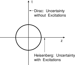
Figure 1: Space-time picture of quantum mechanics. There are quantum excitations along the space-like longitudinal direction, but there are no excitations along the time-like direction. The time-energy relation is a c-number uncertainty relation.

During World War II, Dirac was looking into the possibility of constructing representations of the Lorentz group using harmonic oscillator wave functions [11]. The Lorentz group is the language of special relativity, and the present form of quantum mechanics starts with harmonic oscillators. Presumably, therefore, he was interested in making quantum mechanics Lorentz-covariant by constructing representations of the Lorentz group using harmonic oscillators.

In his 1945 paper [11], Dirac considers the Gaussian form

$$\exp\left\{-{1\over 2}\left(x^{2}+y^{2}+z^{2}+t^{2}\right)\right\}.$$ (19)

We note that this Gaussian form is in the $(x,~{}y,~{}z,~{}t)$ coordinate variables. Thus, if we consider Lorentz boost along the $z$ direction, we can drop the $x$ and $y$ variables, and write the above equation as

$$\exp\left\{-{1\over 2}\left(z^{2}+t^{2}\right)\right\}.$$ (20)

This is a strange expression for those who believe in Lorentz invariance. The expression

$$\exp\left\{-{1\over 2}\left(z^{2}-t^{2}\right)\right\}.$$ (21)

is invariant, but Dirac’s Gaussian form of Eq.(20) is not.

On the other hand, this expression is consistent with his earlier papers on the time-energy uncertainty relation [12]. In those papers, Dirac observes that there is a time-energy uncertainty relation, while there are no excitations along the time axis. He called this the “c-number time-energy uncertainty” relation. When one of us (YSK) was talking with Dirac in 1978, he clearly mentioned this word again. He said further that this is one of the stumbling block in combining quantum mechanics with relativity. This situation is illustrated in Fig. 1.

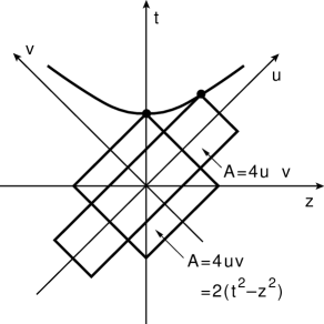
Figure 2: Lorentz boost in the light-cone coordinate system.

Let us look at Fig. 1 carefully. This figure is a pictorial representation of Dirac’s Eq.(20), with localization in both space and time coordinates. Then Dirac’s fundamental question would be how to make this figure covariant? This is where Dirac stops. However, this is not the end of the Dirac story.

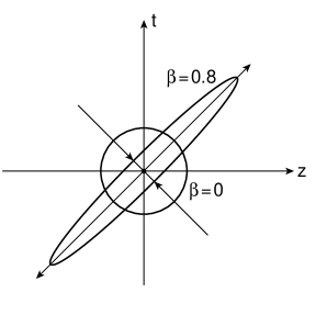
Figure 3: Effect of the Lorentz boost on the space-time wave function. The circular space-time distribution in the rest frame becomes Lorentz-squeezed to become an elliptic distribution.

Dirac’s interest in harmonic oscillators did not stop with his 1945 paper on the representations of the Lorentz group. In his 1963 [13] paper, he constructed a representation of the $O(3,2)$ deSitter group using two coupled harmonic oscillators. This paper contains not only the mathematics of combining special relativity with the quantum mechanics of quarks inside hadrons, but also forms the foundations of two-mode squeezed states which are so essential modern quantum optics [3]. Dirac did not know these when he was writing this 1963 paper.

Furthermore, the $O(3,2)$ deSitter group contains the Lorentz group $O(3,1)$ as a subgroup. Thus, Dirac’s oscillator representation of the deSitter group essentially contains all the mathematical ingredient of what we are doing in this paper.

5 Addendum to Dirac’c Oscillators

In 1949, the Reviews of Modern Physics published a special issue to celebrate Einstein’s 70th birthday. This issue contains Dirac paper entitled “Forms of Relativistic Dynamics” [14]. In this paper, he introduced his light-cone coordinate system, in which a Lorentz boost becomes a squeeze transformation.

When the system is boosted along the $z$ direction, the transformation takes the form

$$\pmatrix{z^{\prime}\cr t^{\prime}}=\pmatrix{\cosh(\eta/2)&\sinh(\eta/2)\cr\sinh(\eta/2)&\cosh(\eta/2)}\pmatrix{z\cr t}.$$ (22)

This is not a rotation, and people still feel strange about this form of transformation. In 1949 [14], Dirac introduced his light-cone variables defined as [14]

$$u=(z+t)/\sqrt{2},\qquad v=(z-t)/\sqrt{2},$$ (23)

the boost transformation of Eq.(22) takes the form

$$u^{\prime}=e^{\eta/2}u,\qquad v^{\prime}=e^{-\eta/2}v.$$ (24)

The $u$ variable becomes expanded while the $v$ variable becomes contracted, as is illustrated in Fig. 2. Their product

$$uv={1\over 2}(z+t)(z-t)={1\over 2}\left(z^{2}-t^{2}\right)$$ (25)

remains invariant. In Dirac’s picture, the Lorentz boost is a squeeze transformation.

If we combine Fig. 1 and Fig. 2, then we end up with Fig. 3. In mathematical formulae, this transformation changes the Gaussian form of Eq.(20) into

$$\psi_{\eta}(z,t)=\left({1\over\pi}\right)^{1/2}\exp\left\{-{1\over 2}\left(e^{-\eta}u^{2}+e^{\eta}v^{2}\right)\right\}.$$ (26)

Let us go back to Sec. 2 on the coupled oscillators. The above expression is the same as Eq.(6). The $x_{1}$ variable now became the longitudinal variable $z$, and the $x_{2}$ variable became the time like variable $t$.

We can use the coupled harmonic oscillators as the starting point of relativistic quantum mechanics. This allows us to translate the quantum mechanics of two coupled oscillators defined over the space of $x_{1}$ and $x_{2}$ into the quantum mechanics defined over the space time region of $z$ and $t$.

This form becomes (20) when $\eta$ becomes zero. The transition from Eq.(20) to Eq.(26) is a squeeze transformation. It is now possible to combine what Dirac observed into a covariant formulation of harmonic oscillator system. First, we can combine his c-number time-energy uncertainty relation described in Fig. 1 and his light-cone coordinate system of Fig. 2 into a picture of covariant space-time localization given in Fig. 3.

In addition, there are two more homework problems which Dirac left us to solve. First, in defining the $t$ variable for the Gaussian form of Eq.(20), Dirac did not specify the physics of this variable. If it is going to be the calendar time, this form vanishes in the remote past and remote future. We are not dealing with this kind of object in physics. What is then the physics of this time-like $t$ variable?

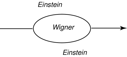
Figure 4: Wigner in Einstein’s world. Einstein formulates special relativity whose energy-momentum relation is valid for point particles as well as particles with internal space-time structure. It was Wigner who formulated the framework for internal space-time symmetries by introducing his little groups whose transformations leave the four-momentum of a given particle invariant.

The Schrödinger quantum mechanics of the hydrogen atom deals with localized probability distribution. Indeed, the localization condition leads to the discrete energy spectrum. Here, the uncertainty relation is stated in terms of the spatial separation between the proton and the electron. If we believe in Lorentz covariance, there must also be a time-separation between the two constituent particles, and an uncertainty relation applicable to this separation variable. Dirac did not say in his papers of 1927 and 1945, but Dirac’s “t” variable is applicable to this time-separation variable. This time-separation variable will be discussed in detail in Sec. 6 for the case of relativistic extended particles.

Second, as for the time-energy uncertainty relation. Dira’c concern was how the c-cnumber time-energy uncertainty relation without excitations can be combined with uncertainties in the position space with excitations. Dira’s 1927 paper was written before Wigner’s 1939 paper on the internal space-time symmetries of relativistic particles.

Both of these questions can be answered in terms of the space-time symmetry of bound states in the Lorentz-covariant regime. In his 1939 paper, Wigner worked out internal space-time symmetries of relativistic particles. He approached the problem by constructing the maximal subgroup of the Lorentz group whose transformations leave the given four-momentum invariant. As a consequence, the internal symmetry of a massive particle is like the three-dimensional rotation group.

If we extend this concept to relativistic bound states, the space-time asymmetry which Dirac observed in 1927 is quite consistent with Einstein’s Lorentz covariance. The time variable can be treated separately. Furthermore, it is possible to construct a representations of Wigner’s little group for massive particles [8]. As for the time-separation, it is also a variable governing internal space-time symmetry which can be linearly mixed when the system is Lorentz-boosted.

6 Feynman’s Oscillators

Quantum field theory has been quite successful in terms of Feynman diagrams based on the S-matrix formalism, but is useful only for physical processes where a set of free particles becomes another set of free particles after interaction. Quantum field theory does not address the question of localized probability distributions and their covariance under Lorentz transformations. In order to address this question, Feynman et al. suggested harmonic oscillators to tackle the problem [15]. Their idea is indicated in Fig. 5.

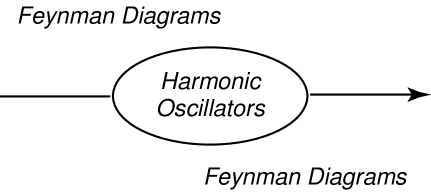
Figure 5: Feynman’s roadmap for combining quantum mechanics with special relativity. Feynman diagrams work for running waves, and they provide a satisfactory resolution for scattering states in Einstein’s world. For standing waves trapped inside an extended hadron, Feynman suggested harmonic oscillators as the first step.

Before 1964 [16], the hydrogen atom was used for illustrating bound states. These days, we use hadrons which are bound states of quarks. Let us use the simplest hadron consisting of two quarks bound together with an attractive force, and consider their space-time positions $x_{a}$ and $x_{b}$, and use the variables

$$X=(x_{a}+x_{b})/2,\qquad x=(x_{a}-x_{b})/2\sqrt{2}.$$ (27)

The four-vector $X$ specifies where the hadron is located in space and time, while the variable $x$ measures the space-time separation between the quarks. According to Einstein, this space-time separation contains a time-like component which actively participates as in Eq.(22), if the hadron is boosted along the $z$ direction. This boost can be conveniently described by the light-cone variables defined in Eq(23). Does this time-separation variable exist when the hadron is at rest? Yes, according to Einstein. In the present form of quantum mechanics, we pretend not to know anything about this variable. Indeed, this variable belongs to Feynman’s rest of the universe.

What do Feynman et al. say about this oscillator wave function? In their classic 1971 paper [15], Feynman et al. start with the following Lorentz-invariant differential equation.

$${1\over 2}\left\{x^{2}_{\mu}-{\partial^{2}\over\partial x_{\mu}^{2}}\right\}\psi(x)=\lambda\psi(x).$$ (28)

This partial differential equation has many different solutions depending on the choice of separable variables and boundary conditions. Feynman et al. insist on Lorentz-invariant solutions which are not normalizable. On the other hand, if we insist on normalization, the ground-state wave function takes the form of Eq.(20). It is then possible to construct a representation of the Poincaré group from the solutions of the above differential equation [8]. If the system is boosted, the wave function becomes given in Eq.(26).

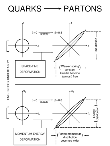
Figure 6: Lorentz-squeezed space-time and momentum-energy wave functions. As the hadron’s speed approaches that of light, both wave functions become concentrated along their respective positive light-cone axes. These light-cone concentrations lead to Feynman’s parton picture.

This wave function becomes Eq.(20) if $\eta$ becomes zero. The transition from Eq.(20) to Eq.(26) is a squeeze transformation. The wave function of Eq.(20) is distributed within a circular region in the $uv$ plane, and thus in the $zt$ plane. On the other hand, the wave function of Eq.(26) is distributed in an elliptic region with the light-cone axes as the major and minor axes respectively. If $\eta$ becomes very large, the wave function becomes concentrated along one of the light-cone axes. Indeed, the form given in Eq.(26) is a Lorentz-squeezed wave function. This squeeze mechanism is illustrated in Fig. 3.

There are many different solutions of the Lorentz invariant differential equation of Eq.(28). The solution given in Eq.(26) is not Lorentz invariant but is covariant. It is normalizable in the $t$ variable, as well as in the space-separation variable $z$. It is indeed possible to construct Wigner’s $O(3)$-like little group for massive particles [17], and thus the representation of the Poincaré group [8]. Our next question is whether this formalism has anything to do with the real world.

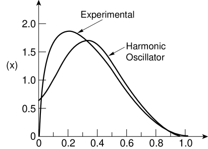
Figure 7: Parton distribution function. Theory and experiment.

In 1969, Feynman observed that a fast-moving hadron can be regarded as a collection of many “partons” whose properties appear to be quite different from those of the quarks [18]. For example, the number of quarks inside a static proton is three, while the number of partons in a rapidly moving proton appears to be infinite. The question then is how the proton looking like a bound state of quarks to one observer can appear different to an observer in a different Lorentz frame? Feynman made the following systematic observations.

• The picture is valid only for hadrons moving with velocity close to that of light.

• The interaction time between the quarks becomes dilated, and partons behave as free independent particles.

• The momentum distribution of partons becomes widespread as the hadron moves fast.

• The number of partons seems to be infinite or much larger than that of quarks.

Because the hadron is believed to be a bound state of two or three quarks, each of the above phenomena appears as a paradox, particularly b) and c) together.

In order to resolve this paradox, let us write down the momentum-energy wave function corresponding to Eq.(26). If we let the quarks have the four-momenta $p_{a}$ and $p_{b}$, it is possible to construct two independent four-momentum variables [15]

$$P=p_{a}+p_{b},\qquad q=\sqrt{2}(p_{a}-p_{b}),$$ (29)

where $P$ is the total four-momentum. It is thus the hadronic four-momentum.

The variable $q$ measures the four-momentum separation between the quarks. Their light-cone variables are

$$q_{u}=(q_{0}-q_{z})/\sqrt{2},\qquad q_{v}=(q_{0}+q_{z})/\sqrt{2}.$$ (30)

The resulting momentum-energy wave function is

$$\phi_{\eta}(q_{z},q_{0})=\left({1\over\pi}\right)^{1/2}\exp\left\{-{1\over 2}\left(e^{\eta}q_{u}^{2}+e^{-\eta}q_{v}^{2}\right)\right\}.$$ (31)

Because we are using here the harmonic oscillator, the mathematical form of the above momentum-energy wave function is identical to that of the space-time wave function. The Lorentz squeeze properties of these wave functions are also the same. This aspect of the squeeze has been exhaustively discussed in the literature [8, 19, 20].

When the hadron is at rest with $\eta=0$, both wave functions behave like those for the static bound state of quarks. As $\eta$ increases, the wave functions become continuously squeezed until they become concentrated along their respective positive light-cone axes. Let us look at the z-axis projection of the space-time wave function. Indeed, the width of the quark distribution increases as the hadronic speed approaches that of the speed of light. The position of each quark appears widespread to the observer in the laboratory frame, and the quarks appear like free particles.

The momentum-energy wave function is just like the space-time wave function, as is shown in Fig. 6. The longitudinal momentum distribution becomes wide-spread as the hadronic speed approaches the velocity of light. This is in contradiction with our expectation from non-relativistic quantum mechanics that the width of the momentum distribution is inversely proportional to that of the position wave function. Our expectation is that if the quarks are free, they must have their sharply defined momenta, not a wide-spread distribution.

However, according to our Lorentz-squeezed space-time and momentum-energy wave functions, the space-time width and the momentum-energy width increase in the same direction as the hadron is boosted. This is of course an effect of Lorentz covariance. This indeed is the key to the resolution of the quark-parton paradox [8, 19].

After these qualitative arguments, we are interested in whether Lorentz-boosted bound-state wave functions in the hadronic rest frame could lead to parton distribution functions. If we start with the ground-state Gaussian wave function for the three-quark wave function for the proton, the parton distribution function appears as Gaussian as is indicated in Fig. 7. This Gaussian form is compared with experimental distribution also in Fig. 7.

For large $x$ region, the agreement is excellent, but the agreement is not satisfactory for small values of $x$. In this region, there is a complication called the “sea quarks.” However, good sea-quark physics starts from good valence-quark physics. Figure 7 indicates that the boosted ground-state wave function provides a good valence-quark physics.

Feynman’s parton picture is one of the most controversial models proposed in the 20th century. The original model is valid only in Lorentz frames where the initial proton moves with infinite momentum. It is gratifying to note that this model can be produced as a limiting case of one covariant model which produces the quark model in the frame where the proton is at rest.

Concluding Remarks

The major strength of the coupled oscillator system is that its classical mechanics is known to every physicist. Not too well known is the fact that this simple device can serve as an analog computer for many of the current problems in physics.

This oscillator system was very useful in illustrating Feynman’s rest of the universe [4]. In this report, we have shown first that the coupled oscillator system can server as an illustrative example of the concept of entanglement, and that Feynman’s rest of the universe is a special case of entanglement. Conversely, the the rest of the universe can be extended to the concept of entanglement.

It was also noted that the coupled-oscillator system provides the mathematical basis for the covariant harmonic oscillators. It can also translate the problems of entanglement to the space and time variables.

It is well known that harmonic oscillators provide bridges between theories. In this paper, we have seen that the coupled harmonic oscillators can serve as a bridge between Dirac and Feynman, and a bridge between coupled oscillators and harmonic oscillators in the Lorentz-covariant world.

References

- [1] S. S. Schweber, An Introduction to Relativistic Quantum Field Theory (Row-Peterson, Elmsford, New York, 1961).
- [2] A. L. Fetter and J. D. Walecka, Quantum Theory of Many Particle Systems (McGraw-Hill, New York, 1971).
- [3] Y. S. Kim and M. E. Noz, Phase Space Picture of Quantum Mechanics (World Scientific, Singapore, 1991).
- [4] D. Han, Y. S. Kim, Am. J. Phys. 67, 61 (1999).
- [5] P. K. Aravind, Am. J. Phys. 57, 309 (1989).
- [6] D. Han, Y. S. Kim, and M. E. Noz, J. Math. Phys. 36, 3940 (1995).
- [7] Y. S. Kim, M. E. Noz, and S. H. Oh, Am. J. Phys. 47, 892 (1979).
- [8] Y. S. Kim and M. E. Noz, Theory and Applications of the Poincaré Group (Reidel, Dordrecht, 1986).
- [9] R. P. Feynman, Statistical Mechanics (Benjamin/Cummings, Reading, MA, 1972).
- [10] E. P. Wigner and M. M. Yanase, 49, 910 (1963). See also J. von Neumann, Die mathematische Grundlagen der Quanten-mechanik (Springer, Berlin, 1932). See also J. von Neumann, Mathematical Foundation of Quantum Mechanics (Princeton University, Princeton, 1955).
- [11] P. A. M. Dirac, Proc. Roy. Soc. (London) A183, 284 (1945).
- [12] P. A. M. Dirac, Proc. Roy. Soc. (London) A114, 234 and 710 (1927).
- [13] P. A. M. Dirac, J. Math. Phys. 4, 901 (1963).
- [14] P. A. M. Dirac, Rev. Mod. Phys. 21, 392 (1949).
- [15] R. P. Feynman, M. Kislinger, and F. Ravndal, Phys. Rev. D 3, 2706 (1971).
- [16] M. Gell-Mann, Phys. Lett. 13, 598 (1964).
- [17] E. Wigner, Ann. Math. 40, 149 (1939).
- [18] R. P. Feynman, The Behavior of Hadron Collisions at Extreme Energies, in High Energy Collisions, Proceedings of the Third International Conference, Stony Brook, New York, edited by C. N. Yang et al., Pages 237-249 (Gordon and Breach, New York, 1969).
- [19] Y. S. Kim and M. E. Noz, Phys. Rev. D 15, 335 (1977).
- [20] Y. S. Kim, Phys. Rev. Lett. 63, 348 (1989).