Information Entropy and Correlation of the Hooke’s Atom

Abstract

We provide an algebraic procedure to find the eigenstates of two-charged particles in an oscillator potential, known as Hooke’s atom. For the planar Hooke’s atom, the exact eigenstates and single particle densities for arbitrary azimuthal quantum number, are obtained analytically. Information entropies associated with the wave functions for the relative motion are then studied systematically, since the same incorporates the effect of the Coulomb interaction. The quantum pottery of the information entropy density reveals a number of intricate structures, which differ significantly for the attractive and repulsive cases. We indicate the procedure to obtain the approximate eigen states. Making use of the relationship of this dynamical system with the quasi-exactly solvable systems, one can also develop a suitable perturbation theory, involving the Coulomb coupling $Z$, for the approximate wave functions.

I Introduction

Interacting charged particles in the presence of a harmonic confinement appears naturally in a number of physical circumstances. For example, two planar charged particles in the presence of a constant magnetic field, interacting ions in a trap are governed by the combined effect of Coulomb and harmonic potentials. Unlike the Coulomb and harmonic cases, the above artificial atom, known as Hooke’s atom is not exactly solvable White ; Kestner ; Laufer ; Wagner . The fact that, a countable infinity of eigenstates can be identified exactly for this case, albeit with differing oscillator frequencies, has made Hooke’s atom a very interesting test ground for checking the effect of correlation arising due to the interaction. The model has been used for explicating the working of density functional theory Sahani . The recent interest in entangled systems, involving continuous variables, makes this model an ideal candidate for a careful study. It should be mentioned that, the comparably simpler system of two-interacting oscillators Moshi have been recently reanalyzed to see the origin of the correlation effects, since in this case both the exact and Hartree-Fock solutions are known March .

After perturbative and numerical investigations of the Hookean atom White ; Kestner ; Laufer ; Wagner , Kais et al., were able to identify one state analytically for a specific value of the spring constant Kais . The same system, with an additional linear term in the inter-particle potential, was also analyzed by Ghosh et al., to study the single particle density Ghosh . Later on, Taut studied this system carefully and through the analysis of the three term recurrence relation showed that, the system possesses analytical solutions for a particular, infinitely denumerable set of oscillator frequencies Taut ; Taut1 ; Turb . He further showed that, two conditions need to be satisfied for obtaining the above solutions. The first one relates the energy with the oscillator frequency and other quantum numbers of the system. The general expression for the second condition, which connects oscillator frequency with the Coulomb coupling and other quantum numbers have not been obtained exactly; the solutions for the first few values have been worked out. Recently Holas et al., have studied the general structure of the density matrix for this system, concentrating on a single value of the spring constant earlier considered by Kais et al March1 .

In this paper, we provide a general algebraic procedure to find the eigenstates of planar Hookean atom, which can be extended to higher dimensions. Our procedure allows one to compute the series expression of the wave function explicitly in a more economic manner as compared to the routinely used series solution approach. It is based on a novel method for obtaining the solutions of linear differential equations pkp ; charan . Apart from obtaining the analytical expressions, in the present approach one can also carry out a perturbative expansion for the wave function, when closed form solutions are not available. The analytical expressions are then used to compute the exact single particle densities for arbitrary values of the quantum numbers. The densities and the information entropy, associated with the pair correlation function are systematically studied to analyze the effect of the interaction on correlation in this artificial atom.

In the following section, we outline the above mentioned method for solving linear differential equations and employ the same to systematically study the eigenstates of the Hooke’s atom. The single particle densities for the planar Hooke’s atom for arbitrary values of azimuthal quantum number are obtained analytically. The single particle densities and information entropy, associated with the relative motion, are then analyzed. The effect of interaction on correlation is shown to be revealed by information entropy. We then point out, how the connection of Hooke’s atom with the well-studied quasi-exactly solvable (QES) system can be used to develop perturbative expansion involving Coulomb coupling parameter $Z$. We conclude in section III after pointing out directions for future studies.

II Hooke’s Atom

The Hooke’s atom, dealing with two interacting charged particles in harmonic potential, is governed by the Hamiltonian (in units, $\hbar=m=e=1$):

$$H=\sum_{i=1}^{2}\left\{\frac{1}{2}\left({\bf{p}}_{i}+\frac{1}{c}{\bf{A(r_{i})}}\right)^{2}+\frac{1}{2}\omega_{0}^{2}r_{i}^{2}\right\}+\frac{Z}{|{\bf{r}}_{2}-{\bf{r}_{1}|}}.$$ (1)

This Hamiltonian decouples in the center of mass ${\bf{R}}=\frac{1}{2}({\bf{r}}_{1}+{\bf{r}}_{2})$ and the relative coordinate, ${\bf{r}}={\bf{r}}_{2}-{\bf{r}}_{1}$, which give rise to the new momentum operators, ${{\bf{p}}=-i\bf{\nabla}}_{r}=\frac{1}{2}\left({\bf{p}}_{2}-{\bf{p}}_{1}\right)$ and ${\bf{P}}=-i{\bf{\nabla}}_{R}={\bf{p}}_{2}+{\bf{p}}_{1}$.

Eq.(1) in these coordinates reads

$$H = 2\left\{\frac{1}{2}\left[{\bf{p}}+\frac{1}{c}{\bf{A_{r}}}\right]^{2}+\frac{1}{2}\omega_{r}r^{2}+\frac{Z}{2r}\right\}+\frac{1}{2}\left\{\frac{1}{2}\left[{\bf{P}}+\frac{1}{c}{\bf{A_{R}}}\right]^{2}+\frac{1}{2}\omega_{R}R^{2}\right\}~{},$$ (2)

$$\equiv 2H_{r}+\frac{1}{2}H_{R}$$ (3)

where ${\bf{A_{R}}}=2{\bf{A(R)}}={\bf{A}(\bf{r}_{1})}+{\bf{A}(\bf{r}_{2})}$, ${\bf{A_{r}}}=\frac{1}{2}{\bf{A(r)}}=\frac{1}{2}({\bf{A}(\bf{r}_{2})}-{\bf{A}(\bf{r}_{1})})$ and $\omega_{R}=2\omega_{0}$, $\omega_{r}=\frac{1}{2}\omega_{0}$. The total wave function factorizes:

$$\Psi(1,2)=\xi({\bf{R}})\varphi({\bf{r}})~{}.$$ (4)

It is clear from Eq.(3) that, the eigenstates of $H_{R}$ are identical with the two dimensional oscillator states, where ${\bf{A_{R}}}$ is a linear function of $R$, for a constant magnetic field $B$.

The Schrödinger equation $H_{r}\varphi({\bf{r}})=\varepsilon\varphi({\bf{r}})$ for the internal motion, can be cast in the form,

$$\left\{-\frac{1}{2}\left[r^{-1/2}\frac{\partial^{2}}{\partial r^{2}}r^{1/2}+\frac{1}{r^{2}}\left(\frac{\partial^{2}}{\partial\phi^{2}}+\frac{1}{4}\right)\right]-\frac{i\omega_{L}}{2}\frac{\partial}{\partial\phi}+\frac{1}{2}\left[\omega_{r}^{2}+\frac{1}{4}\omega_{L}^{2}\right]r^{2}+\frac{Z}{2r}\right\}\varphi(\bf{r})=\varepsilon\varphi(\bf{r}).$$ (5)

Here $\omega_{L}$ is the Larmor frequency. The angular and radial part of the wave function $\varphi(\bf{r})$, are decoupled through the ansatz,

$$\varphi({\bf{r}})=\frac{e^{im\phi}}{\sqrt{2\pi}}\frac{u(r)}{r^{1/2}}~{}~{}~{}~{}~{}m=0,\pm 1,\pm 2,\cdots,$$ (6)

where $u(r)$ satisfies the radial equation,

$$\left\{-\frac{1}{2}\frac{d^{2}}{dr^{2}}+\frac{1}{2}\left(m^{2}-\frac{1}{4}\right)\frac{1}{r^{2}}+\frac{1}{2}\tilde{\omega}_{r}^{2}r^{2}+\frac{Z}{2r}\right\}u(r)=\left[\varepsilon-\frac{1}{2}m\omega_{L}\right]u(r).$$ (7)

Here $\tilde{\omega}_{r}=\frac{1}{2}\sqrt{\omega_{L}^{2}+\omega_{0}^{2}}$. To solve the above equation, one introduces the dimensionless variable $\rho=\sqrt{\tilde{\omega}_{r}}~{}r$ and

$$\varepsilon^{\prime}=\frac{2}{\tilde{\omega}_{r}}\left(\varepsilon-\frac{1}{2}m\omega_{L}\right)~{},$$ (8)

and substitute

$$u=e^{-\frac{1}{2}\rho^{2}}\rho^{|m|+1/2}t(\rho)~{}.$$ (9)

This yields the following equation:

$$\left\{\frac{d^{2}}{d\rho^{2}}-2\rho\frac{d}{d\rho}+2\left(|m|+\frac{1}{2}\right)\frac{1}{\rho}\frac{d}{d\rho}-\frac{Z}{\sqrt{\tilde{\omega}_{r}}\rho}+\left(\varepsilon^{\prime}-2|m|-2\right)\right\}t(\rho)=0~{}.$$ (10)

The above radial equation can be solved for a series solution, following a recently developed method for solving linear differential equations pkp ; charan . A single variable differential equation, after suitable manipulations, can be cast in the form,

$$\left[F(D)+P(x,d/dx)\right]y(x)=0~{}~{};$$ (11)

here $F(D)$ is a function of the Euler operator $D\equiv x\frac{d}{dx}$, possibly containing a constant. $P(x,d/dx)$ contains other operators of the differential equation concerned. The series solution for $y(x)$ can be written in the form:

$$y(x)=C_{\l}\left\{\sum_{\nu=0}^{\infty}(-1)^{\nu}\left[\frac{1}{F(D)}P(x,d/dx)\right]^{\nu}\right\}x^{\l},$$ (12)

provided $F(D)x^{\l}=0$.

The proof of this can be be checked by direct substitution. For the Hooke’s atom case, we have $F(D)\equiv D(D+2m)$, $\l=0,-2m$ and $P\equiv\left(\varepsilon^{\prime}-2|m|-2\right)\rho^{2}-2\rho^{3}\frac{d}{d\rho}-\frac{Z\rho}{\sqrt{\tilde{\omega}_{r}}}$, after multiplying $\rho^{2}$ to the Eq.(10). Eq.(12) yields,

$$t(\rho)=C_{0}\left\{\sum_{\nu=0}^{\infty}(-1)^{\nu}\left[\frac{1}{D(D+2m)}\left\{\left(\varepsilon^{\prime}-2|m|-2\right)\rho^{2}-2\rho^{3}\frac{d}{d\rho}-\frac{Z\rho}{\sqrt{\tilde{\omega}_{r}}}\right\}\right]^{\nu}\right\}\rho^{0}~{},$$ (13)

which can be expanded in the form,

$$t(\rho) = 1+\frac{Z}{{\sqrt{\tilde{\omega}_{r}}}(2m+1)}\rho+\left(\frac{Z^{2}}{\tilde{\omega}_{r}(2m+1)2(2m+2)}-\frac{\tilde{E}}{2(2m+2)}\right)\rho^{2}$$ (14)

$$+ \frac{1}{\sqrt{\tilde{\omega}}_{r}}\left\{\frac{Z^{3}}{\tilde{\omega}_{r}(2m+1)2(2m+2)3(2m+3)}-\frac{Z\tilde{E}}{(2m+1)3(2m+3)}\right.$$

$$+ \left.\frac{Z\tilde{E}}{2(2m+2)3(2m+3)}-\frac{2Z}{(2m+1)3(2m+3)}\right\}\rho^{3}+\cdots~{}~{},~{}~{}{\mathrm{here}}~{}~{}\tilde{E}=\varepsilon^{\prime}-2(|m|+1)~{}.$$

In order that, the above series terminates at $\rho^{n-1}$, the coefficients of $\rho^{n}$ and $\rho^{n+1}$ terms must be zero. There are two operators $\left\{\left(\varepsilon^{\prime}-2|m|-2\right)\rho^{2}-2\rho^{3}\frac{d}{d\rho}\right\}$ and $\frac{Z\rho}{\sqrt{\tilde{\omega}_{r}}}$, which increase the degree of the polynomial solution. Once $a_{n}$, the coefficient of $\rho^{n}$ is zero, $\rho^{n+1}$ term will not get any contribution from $\frac{Z\rho}{\sqrt{\tilde{\omega}_{r}}}$ and the only contribution to $a_{n+1}$ will arise from the action of $\left\{\left(\varepsilon^{\prime}-2|m|-2\right)\rho^{2}-2\rho^{3}\frac{d}{d\rho}\right\}$ on $a_{n-1}\rho^{n-1}$. Hence, $a_{n+1}=0$ yields, $\varepsilon^{\prime}=2(n+|m|)$. The coefficients $a_{n}$ can be straightforwardly determined in our approach; although it becomes tedious for higher values of $n$. Once the above condition is implemented, one needs to check if $a_{n}=0$ yields exact solutions.

For $n=2$ and arbitrary $m$ and $Z$, we have the frequencies

$$\tilde{\omega}_{r}=\frac{Z^{2}}{2(2|m|+1)}~{}~{}{\mathrm{and~{}~{}energy}}~{}~{}\varepsilon=\frac{Z^{2}(|m|+2)}{(2|m|+1)}+\frac{1}{2}m\omega_{L}$$

and

$$u(r)=1+\frac{Zr}{(2|m|+1)}.$$ (15)

For $n=3$ and arbitrary $m$ and $Z$, we have the frequencies

$$\tilde{\omega}_{r}=\frac{Z^{2}}{4(4|m|+3)}~{}~{}{\mathrm{and~{}~{}energy}}~{}~{}\varepsilon=\frac{Z^{2}(|m|+2)}{2(4|m|+3)}+\frac{1}{2}m\omega_{L}$$

and

$$u(r)=1+\frac{Zr}{(2|m|+1)}+\frac{Z^{2}r^{2}}{2(2m+1)(4m+3)}.$$ (16)

In case of $n=4$, we have two roots for the oscillator frequency:

$$\tilde{\omega}_{r}=\frac{10Z^{2}+10Z^{2}|m|\pm Z^{2}{\sqrt{73+128|m|+64|m|^{2}}}}{18(4|m|^{2}+8|m|+3)}~{}~{}.$$

For the lower frequency the polynomial part of the wave function is given by,

$$u(r) = 1+\frac{Zr}{(2|m|+1)}+\frac{Z^{2}\left({\sqrt{73+128|m|+64|m|^{2}}}-4|m|-1\right)}{12(|m|+1)(4|m|^{2}+8|m|+3)}r^{2}$$ (17)

$$+ \frac{Z^{3}\left(11{\sqrt{73+128|m|+64|m|^{2}}}+2|m|(7{\sqrt{73+128|m|+64|m|^{2}}}-89)-104|m|^{2}-83\right)}{108(|m|+1)(4|m|^{2}+8|m|)^{2}}r^{3},$$

with energy $\varepsilon=2(n+|m|){\tilde{\omega}}_{r}$. The other eigenvalues and eigenstates can be found analogously. We note that, for the general case the coefficients of $\rho^{n+1}$ yields a relation between the energy, frequency and the azimuthal quantum number. It is the second relationship i.e., $a_{n}=0$ which brings the relationship between $Z$, $\tilde{\omega}_{r}$ and $m$. It is worth mentioning that, using the above series expansion, it is possible to approximately determine the other analytically inaccessible states of a given Hamiltonian. Although, we intend to deal with this in greater detail later, below we briefly outline the underlying procedure. To be specific, consider the repulsive $n=2$ case, for which the ground state is analytically available for a particular frequency. To obtain approximately, the first excited state of the same Hamiltonian, one starts with the above series expansion, retaining sufficient number of terms to ensure that the wave function has one real zero in the half line. In this wave function the energy can be treated as a variational parameter, to accurately determine the eigenvalue and eigen state, as has been shown for the QES sextic oscillator previously Atre . This process will be made more transparent while demonstrating the connection of the Hooke’s atom with the above mentioned sextic oscillator problem below.

We now proceed to compute the pair correlation function and single particle density defined respectively as,

$$G({\bf{r}})=\left\langle\Psi{\left|\sum_{i<j}\delta({\bf{r}}_{i}-{\bf{r}}_{j}-{\bf{r}})\right|}\Psi\right\rangle=|\varphi({\bf{r}})|^{2},$$ (18)

$$n({\bf{r}})=\left\langle\Psi{\left|\sum_{i=1}^{2}\delta({\bf{r}}-{\bf{r}}_{i})\right|}\Psi\right\rangle~{}.$$ (19)

The expression for the charge density for $n=2$, $m=0$ and $Z=1$ can be computed:

$$n({\bf{r}})= \frac{1}{125(3+\sqrt{2\pi})}$$ (20)

$$\times \left[16e^{-\frac{9r^{2}}{20}}\pi^{3}\left\{e^{\frac{r^{2}}{20}}\left(65+4r^{2}\right)+{\sqrt{10\pi}\left(10+r^{2}\right)I_{0}\left(\frac{r^{2}}{20}\right)}+{\sqrt{10\pi}}r^{2}I_{1}\left(\frac{r^{2}}{20}\right)\right\}\right]~{}~{}.$$

The corresponding attractive case ($Z=-1$) is given by:

$$n({\bf{r}})= \frac{1}{125(3-\sqrt{2\pi})}$$ (21)

$$\times \left[16e^{-\frac{9r^{2}}{20}}\pi^{3}\left\{e^{\frac{r^{2}}{20}}\left(65+4r^{2}\right)-{\sqrt{10\pi}\left(10+r^{2}\right)I_{0}\left(\frac{r^{2}}{20}\right)}-{\sqrt{10\pi}}r^{2}I_{1}\left(\frac{r^{2}}{20}\right)\right\}\right]~{}~{}.$$

Similarly for the repulsive case, with $m=1$, we have

$$n({\bf{r}})=\frac{1}{9375(42+9\sqrt{6\pi})}\left[64e^{-\frac{3r^{2}}{20}}\pi^{3}\left\{e^{\frac{r^{2}}{60}}\left(13950+705r^{2}+4r^{4}\right)\right.\right.$$

$$\left.\left.+{\sqrt{30\pi}\left(1350+90r^{2}+r^{4}\right)I_{0}\left(\frac{r^{2}}{60}\right)}+{\sqrt{30\pi}}r^{2}\left(60+r^{2}\right)I_{1}\left(\frac{r^{2}}{60}\right)\right\}\right].$$ (22)

For $n=3$, $Z=1$ and $m=0$,

$$n({\bf{r}})=\frac{1}{28125(25+8\sqrt{3\pi})}\left[16e^{-\frac{3r^{2}}{40}}\pi^{3}\left\{e^{\frac{r^{2}}{120}}\left(106425+2160r^{2}+4r^{4}\right)\right.\right.$$

$$\left.\left.-{\sqrt{15\pi}\left(15300+435r^{2}+2r^{4}\right)I_{0}\left(\frac{r^{2}}{120}\right)}-{\sqrt{15\pi}}r^{2}\left(315+2r^{2}\right)I_{1}\left(\frac{r^{2}}{120}\right)\right\}\right]~{}~{}.$$ (23)

We give below the three dimensional plots of information entropy densities associated with the pair correlation function $G({\bf{r}})=|\varphi({\bf{r}})|^{2}$, as the same incorporates the interaction, defined as $S_{G}({\bf{r}})=-G({\bf{r}})\ln[G({\bf{r}})]$, for various values of $n$ and Coulomb couplings. The effect of interaction on the correlation is clearly seen in these plots. In Fig.1 we have plotted $S_{G}({\bf{r}})$ for $n=2$, $Z=-1$ and various values of azimuthal quantum number $m=0,1$ and $2$. We observe a dip at the origin; this occurs because $G({\bf{r}})>1$ at $r=0$ which makes the quantity $S_{G}({\bf{r}})<0$. This is a special case, as for higher $n$ values and $m=0$, we observe a peak at the origin, since $G({\bf{r}})<1$. For higher values of $m$ correlation decreases and wave function of the system delocalizes. Similar behavior is seen in Fig.2. Fig. 3 explicates the effect of Coulomb interaction on the entropy density; Fig.3 (a), (b) and (c) are plotted for various coupling strengths keeping $n$ and $m$ fixed. It is clear that, as the coupling strength increases, the system becomes more localized. In Fig. 4, we have plotted the entropy density for repulsive Hooke’s atom with $n=4$. We observe, for the $m=0$ there is a small dip at the center, which becomes wider for higher values of $m$, which agrees with the fact that for higher values of $m$ there is less correlation present in the system.

In Fig. 5, we have numerically calculated the position space entropy for various values of $m$, keeping $n=3$, for attractive and repulsive cases. It is clear from the plot that, as the oscillator frequency increases (which corresponds to a smaller value of $m$), entropy decreases. Also an attractive system has more entropy as compared to its repulsive counterpart.

The Hooke’s atom can be connected to the quasi-exactly solvable models by a simple coordinate transformation. We can make use of this connection to develop a suitable perturbation theory involving the coupling parameter $Z$. The QES systems are intermediate to exactly solvable and non-solvable systems. Unlike the exactly solvable models, in such systems only a finite number of states can be determined analytically Shifm ; Ushve . The typical example of a QES system, which we are going to map with Hooke’s atom is a sextic oscillator with a centrifugal barrier, whose Hamiltonian is given by,

$$\hat{H}=-\frac{1}{2}\frac{d^{2}}{dx^{2}}+\frac{\alpha x^{2}}{2}+\frac{\gamma x^{6}}{2}+\frac{m(m+1)}{2x^{2}}~{}~{}.$$ (24)

We make the following similarity transformation $\tilde{H}=\psi_{0}^{-1}(x)\hat{H}\psi_{0}(x)$, with $\psi_{0}(x)=x^{m+1}\exp(-x^{4}{\sqrt{\gamma}}/4)$ and seek the polynomial solution for the reduced Hamiltonian,

$$\tilde{H}=-\frac{1}{2}\frac{d^{2}}{dx^{2}}+\sqrt{\gamma}x^{3}\frac{d}{dx}+\left(\frac{\alpha}{2}+\frac{3\sqrt{\gamma}}{2}+(m+1)\sqrt{\gamma}\right)x^{2}-(m+1)\frac{1}{x}\frac{d}{dx}~{}~{}.$$ (25)

The series solution of the above equation, in the present approach, can be written for $F(D)\equiv D(D+2m+1)$:

$$u(x) = C_{0}\sum_{\nu=0}^{\infty}\left\{(-1)^{\nu}\left[\frac{1}{F(D)}\left(Ex^{2}-Ax^{4}-2\sqrt{\gamma}x^{5}\frac{d}{dx}\right)\right]^{\nu}\right\}x^{0},$$ (26)

$$u(x) = 1-\frac{E}{2(2m+3)}x^{2}+\left\{\frac{A}{4(2m+5)}+\frac{E^{2}}{2(2m+3)4(2m+5)}\right\}x^{4}$$ (27)

$$- \left\{\frac{E^{3}}{2(2m+3)4(2m+5)6(2m+7)}+\frac{EA}{4(2m+5)6(2m+7)}+\frac{EA}{2(2m+3)6(2m+7)}+\frac{4E\sqrt{\gamma}}{2(2m+3)6(2m+7)}\right\}x^{6}+\cdots~{},$$

where, $A=\left(\frac{\alpha}{2}+\frac{3\sqrt{\gamma}}{2}+(m+1)\sqrt{\gamma}\right).$

It is worth noting that, the operators in the above equation, $\sqrt{\gamma}x^{3}\frac{d}{dx}$ and $\left(\frac{\alpha}{2}+\frac{3\sqrt{\gamma}}{2}+(m+1)\sqrt{\gamma}\right)x^{2}$ increase the degree of the polynomial by two. In order to preserve the degree of the polynomial in an eigenvalue equation of $\tilde{H}$, the following condition on the parameters should be imposed,

$$\frac{\alpha}{2}+\frac{3\sqrt{\gamma}}{2}+(m+1)\sqrt{\gamma}=-n\sqrt{\gamma}~{}~{}.$$ (28)

A simple transformation of variable: $x^{2}=r$ in Eq.(24) allows us to map this QES problem to Hooke’s atom;

$$\left[-\frac{1}{2}\left\{4r\frac{d^{2}}{dr^{2}}+2\frac{d}{dr}\right\}+\frac{\alpha r}{2}+\frac{\gamma r^{3}}{2}+\frac{m(m+1)}{2r}\right]\psi(r)=E\psi(r)~{}~{},$$

$${\mathrm{or}}~{}~{}\left[-\frac{d^{2}}{dr^{2}}-\frac{1}{2r}\frac{d}{dr}+\frac{\gamma}{4}r^{2}+\frac{m(m+1)}{4r^{2}}-\frac{E}{2r}\right]\psi(r)=-\frac{\alpha}{4}\psi(r)~{}~{}.$$ (29)

With $\psi(r)=r^{-1/4}\varphi(r)$ and $(\tilde{m}^{2}-1/4)=\frac{m(m+1)}{4}-\frac{3}{16}$ the above equation, comes to the form of Hooke’s atom,

$$\left[-\frac{1}{2}\frac{d^{2}}{dr^{2}}+\frac{\gamma}{8}r^{2}+\frac{1}{2}\left(\tilde{m}^{2}-\frac{1}{4}\right)\frac{1}{r^{2}}-\frac{E}{4r}\right]\psi(r)=-\frac{\alpha}{8}\psi(r).$$ (30)

It is interesting to notice that, energy eigenvalue, quadratic and sextic couplings of the QES Hamiltonian become the Coulomb coupling, energy and quadratic coupling of the corresponding Hookean system respectively, but the centrifugal barrier term remains same in both the cases. With this parameterization, it can be easily seen that the QES condition given by Eq.(28) is same as the reduced energy $\varepsilon^{\prime}=2(n+|m|)$. As has been mentioned earlier, for finding the analytically inaccessible QES states, one can start with the above series expansion and terminate it at a desired degree, depending on the required number of the nodes of the concerned wave function. Treating energy as a variational parameter, one minimizes $\langle\Psi|(H-E)|\Psi\rangle$, to obtain an accurate expression for the eigen state and eigen value Atre . The perturbation in energy in QES regime implies a perturbation in $Z$ in its Hookean counterpart.

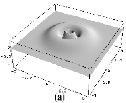
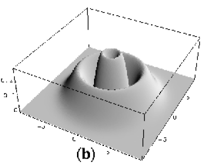
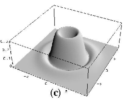
Figure 1: Plots of information entropy density for attractive $Z=-1$ planar Hooke’s atom with $n=2$ and (a) $m=0$, (b) $m=1$ and (c) $m=2$.

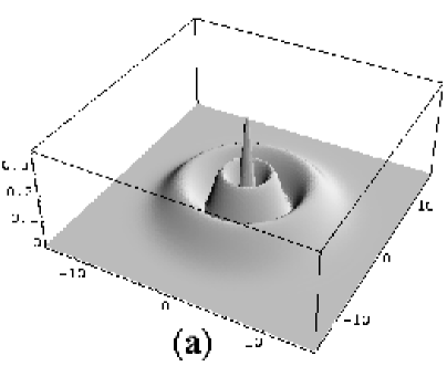
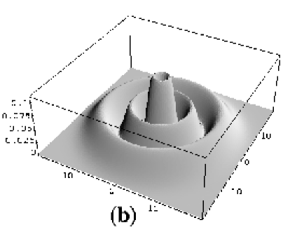
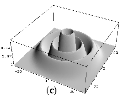
Figure 2: Plots of information entropy density for attractive $Z=-1$ planar Hooke’s atom with $n=3$ and (a) $m=0$, (b) $m=1$ and (c) $m=2$.

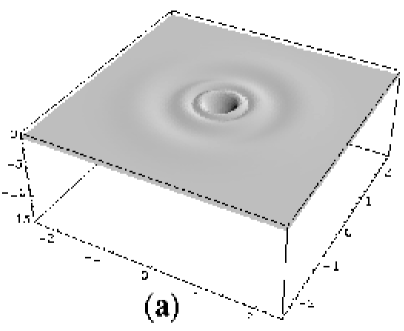
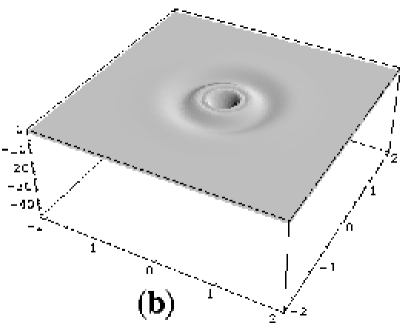
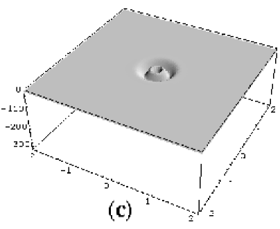
Figure 3: Plots of information entropy density for attractive planar Hooke’s atom with $n=2$ and $m=0$ depicting the effect of Coulomb coupling strength for (a) $Z=-2$, (b) $Z=-3$ and (c) $Z=-7$.

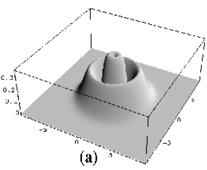
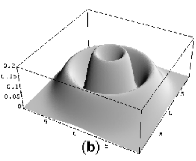
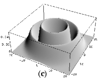
Figure 4: Plots of information entropy density for repulsive ($Z=1$) planar Hooke’s atom with $n=4$ (a) $m=0$, (b) $m=1$ and (c) $m=5$.

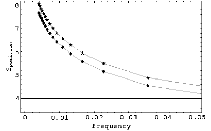
Figure 5: Plot depicting the variation of position space entropy with respect to various allowed oscillator frequencies for $n=3$, the green line and red lines are for attractive and repulsive cases respectively.

III Conclusions

In conclusion, we have illustrated the utility of a recently developed method for solving linear differential equations to Hooke’s atom The information entropy and their densities are analyzed systematically for studying the effect of interaction on correlation. The procedure for developing perturbative expansions based on the present approach is indicated. A connection of this dynamical system with well studied QES systems can also be used for developing a suitable perturbation theory involving the charge parameter $Z$. The usefulness of single particle density to density functional theory is well-known, as also its ability for studying entanglement of this correlated system. We would like to get back to these questions in near future. Recently, Ralko and Truong Truong1 has connected this system to anyons and Heun’s equation heun . This is an interesting direction, needing further investigations.

Acknowledgments: We acknowledge many useful discussions with Prof. K.D. Sen, who also brought to our notice many relevant references. CSM thanks Physical Research Laboratory for the hospitality during this project.

References

• (1)
• (2) D. Fu-Tai Tuan, J. Chem. Phys. 50, 2740 (1969);
R.J. White and W. Byres Brown, ibid. 53, 3869 (1970);
J.M. Benson and W. Byres Brown, ibid. 53, 3880 (1970).
• (3) N.R. Kestner and O. Sinanoḡlu, Phys. Rev. 128, 2687 (1962).
• (4) P.M. Laufer and J. B. Krieger, Phys. Rev. A 33, 1480 (1986).
• (5) U. Merkt, J. Huser and M. Wagner, Phys. Rev. B 43, 7320 (1991).
• (6) Z. Qian and V. Sahni, Phys. Rev. A 57, 2527 (1998).
• (7) M. Moshinsky, Am. J. Phys. 36, 52 (1968).
• (8) C. Amovilli and N.H. March, Phys. Rev. A 69, 054302 (2004).
• (9) S. Kais, D.R. Herschbach and R.D. Levine, J. Chem. Phys. 91, 7791 (1989).
• (10) S.K. Ghosh and A. Samanta, J. Chem. Phys. 94, 517 (1991).
• (11) M. Taut, Phys. Rev. A 48, 3561 (1993).
• (12) M. Taut, J. Phys. A: Math. Gen. 27, 1045 (1994).
• (13) A. Turbiner, Phys. Rev. A 50, 5335 (1994).
• (14) A. Holas, I.A. Howard and N.H. March, Phys. Lett. A 310, 451 (2003).
• (15) N. Gurappa and P.K. Panigrahi, Phys. Rev. B 62, 1943 (2000).
• (16) N. Gurappa, P.K. Panigrahi and T. Shreecharan, J. Comput. Appl. Math. 160, 103 (2003).
• (17) R. Atre and P.K. Panigrahi, Phys. Lett. A 317, 46 (2003).
• (18) M.A. Shifman, Int. J. Mod. Phys. A 4, 2897 (1989) and references therein.
• (19) A. Ushveridze, Quasi-Exactly Solvable Models in Quantum Mechanics (Inst. of Physics Publishing, Bristol, 1994) and references therein.
• (20) A. Ralko and T.T Truong, Phys. Lett. A 323, 395 (2004).
• (21) N. Gurappa and P.K. Panigrahi, On polynomial solutions of Heun equation, to appear in J. Phys. A. Math. Gen., math-ph/0410015.