Entanglement Across a Transition to Quantum Chaos

Abstract

We study the relation between entanglement and quantum chaos in one- and two-dimensional spin-$1/2$ lattice models, which exhibit mixing of the noninteracting eigenfunctions and transition from integrability to quantum chaos. Contrary to what occurs in a quantum phase transition, the onset of quantum chaos is not a property of the ground state but take place for any typical many-spin quantum state. We study bipartite and pairwise entanglement measures, namely the reduced Von Neumann entropy and the concurrence, and discuss quantum entanglement sharing. Our results suggest that the behavior of the entanglement is related to the mixing of the eigenfunctions rather than to the transition to chaos.

I Introduction

Quantum entanglement has been identified as a key ingredient in quantum communication and information processing. The content of entanglement in a particular system is considered as a resource to perform several tasks in a more efficient and more secure way than any other classical method chuang00 ; benenti04 . For instance, quantum teleportation protocols require to share a maximally entangled state between the sender and the receiver. In the field of quantum computation, it has been found that for the case of quantum algorithms operating on pure states, the presence of multipartite entanglement between the components constituting a quantum processor is a necessary condition to achieve an exponential speedup over classical computation linden02 .

On the other hand, for the operability and stability of any quantum computer, the entanglement can also play the role of the property to be minimized. The unavoidable entanglement between the quantum processor and the environment is one of the most important sources of noise and, therefore, of computational errors. The understanding and control of noise in quantum protocols is clearly needed to implement any reliable quantum computation paz ; zurek ; song ; carlo ; rossini03 ; facchi . Even when a quantum processor is ideally isolated from the environment, i.e., in situations where the decoherence time of the processor is very large as compared to the computational time scales, the operability of the quantum computer is not yet guaranteed georgeot00 . Indeed, also the presence of device imperfections hinders the implementation of any quantum computation. A quantum computer is a quantum many-body system. The interaction between the qubits composing the quantum registers of the computer is needed to produce the necessary amount of entanglement. Moreover, device imperfections like small inaccuracy in the coupling constants induce errors. Above a certain imperfection strength threshold (chaos border), quantum chaos sets in georgeot00 ; flambaum ; benenti01 ; berman01 . In such a regime, exponentially many states of the computational basis are mixed after a chaotic time scale. This sets an upper time limit to the stability of a generic superposition of states coded in the quantum computer wave function. A necessary requirement for quantum computer operability and fault tolerant computation schemes is the possibility to operate many quantum gates inside the chaotic time scale.

For the case of many-body systems, the transition to chaos has been studied for fermions and bosons (see e.g. many-bodies and references therein), and particularly for lattice spin systems spin-systems . In fermionic systems with two-body interactions it has been found that, if the interaction strength exceeds some critical value, fast transition to chaos occurs in the Hilbert space of many-particle states izrailev99 . This is commonly studied in terms of the transition between the different spectral statistics of integrable and chaotic systems. For systems with a finite size, this transition is smooth and only a crossover border where the transition occurs can be identified. The question whether this smooth transition becomes sharp in the thermodynamic limit is still under debate. However, in some cases a sharp transition to chaos is found, e.g., in the three-dimensional Anderson model 3D-anderson .

In a different context, the behavior of quantum entanglement across a quantum phase transition has recently attracted much attention. Quantum phase transitions (QPT) consist in a qualitative change in the ground state of the system as some control parameter is varied sachdev . Unlike classical phase transitions, QPT occur at zero temperature and the fluctuations developed at the critical point are fully quantum. These fluctuations dominate the behavior of the system near the critical point, where correlations are long-range in character. It has been recently pointed out that the genuine quantum character of quantum phase transitions is due to entanglement osborne01 . It has also been argued that the ground state of the system is strongly entangled at the critical point osborne01 ; volya03 . Therefore, the behavior of entanglement across QPT is particularly interesting for quantum computation and communication, where a maximization of the content of entanglement is desirable. The study of the relation between QPT and entanglement has been focused on the possible universal behavior of the entanglement content at the transition fazio02 ; osborne02 ; bose02 ; vidal03 ; gu03 ; glaser03 ; korepin04 ; mosseri04 ; cirac04 . In this context, it has been shown that in different model systems quantities like the derivative of the concurrence fazio02 ; osborne02 and Von Neumann entropy vidal03 ; latorre-S present critical behavior at the transition. The dependence of entanglement on disorder and its interplay with chaos has also been studied simone ; santos03 ; emary04 . Moreover, the evolution of entanglement in quantum algorithms simulating quantum chaos has been recently investigated bettelli03 ; caves ; lahiri03 ; hu03-1 .

The aim of this paper is to characterize the behavior of quantum entanglement in non-integrable systems when a transition to quantum chaos occurs. We are interested in understanding how the entanglement content behaves in transitions from integrability to chaos. We would like to stress that, differently from the previous studies on QPT fazio02 ; osborne02 ; bose02 ; vidal03 ; gu03 ; glaser03 ; korepin04 ; mosseri04 ; cirac04 , the transition to chaos is not only a property of the ground state but takes place for any typical many-body state. We numerically study two lattice models of interacting many spins that show a transition to chaos. They have previously been studied as models of the quantum computer hardware georgeot00 ; flambaum ; benenti01 ; berman01 . In both models, the transition to chaos is driven by the strength of the interaction between the spins. We consider bipartite and pairwise entanglement measures and focus on the relation between the entanglement and the onset of chaos. We focus our study on the eigenstates corresponding to the center of the spectrum, where the many-body density of states is larger and therefore quantum chaos sets in at small interaction strengths. Nevertheless, also the behavior of the other parts of the spectrum is discussed. We use exact diagonalization techniques to obtain all the eigenstates of the considered spin models. Therefore, we are limited to consider relatively small system sizes, from which the study of any possible finite-size scaling for the behavior of the entanglement at the chaos border is out of reach. Nevertheless, we discuss, at a qualitative level, the similarities and differences between the behavior of entanglement across a QPT and at the onset of quantum chaos. We show that the dependence of pairwise entanglement on the size, distance and range of the interactions can be understood in terms of the sharing of entanglement among the different parties of the system. Furthermore, we demonstrate that the behavior of entanglement is related to the mixing of noninteracting eigenfunctions rather than to the transition to chaos.

This paper is organized as follows. In Sec. II we review the measures of entanglement that we will use. The measures that signal the onset of quantum chaos are reviewed in Sec. III. In Sec. IV we define the spin lattice models investigated in this paper and discuss numerical results on their entanglement content and their transition to chaos. In Sec. V we present our final remarks.

II Measures of Entanglement

A pure state ${|\psi\rangle}$ is said to be separable if for a given partition of its Hilbert space ${\mathcal{H}}={\mathcal{H}}_{A}\otimes{\mathcal{H}}_{B}$ it can be written as ${|\psi\rangle}={|a\rangle}\otimes{|b\rangle}$. Here ${|a\rangle}$ and ${|b\rangle}$ are vectors residing in the Hilbert subspaces ${\mathcal{H}}_{A}$ and ${\mathcal{H}}_{B}$, respectively. The pure state ${|\psi\rangle}$ is entangled if it is not separable.

II.1 Von Neumann entropy

Pure bipartite entanglement is measured in terms of the reduced Von Neumann entropy $S$. For a pure state the reduction of its density matrix $\rho={|\psi\rangle}{\langle\psi|}$ is obtained through partial trace of one the two partitions as $\rho_{A}=\mathrm{tr}_{B}\rho$ or, equivalently, $\rho_{B}=\mathrm{tr}_{A}\rho$. Then, $S$ is defined as

$$S=S_{A}=S_{B}=-\mathrm{tr}_{B}(\rho_{B}\log\rho_{B})\ .$$ (1)

The Von Neumann entropy provides an unambiguous measure of entanglement for a bipartite system in an overall pure state. For a separable state $S=0$ while for a maximally entangled state $S=\log{\mathcal{N}}$, where ${\mathcal{N}}=\min({{\mathcal{N}}_{A},{\mathcal{N}}_{B}})$, with ${\mathcal{N}}_{A}={\rm dim}({\mathcal{H}}_{A})$ and ${\mathcal{N}}_{B}={\rm dim}({\mathcal{H}}_{B})$. In what follows we will take the logarithm in Eq. (1) base $2$. Thus, for a many-qubit system, the maximum value that the Von Neumann entropy can take is equal to the number of qubits that have not been traced out to obtain the reduced density matrix.

II.2 Concurrence and entanglement of formation

For the case of mixed states, the Von Neumann entropy is no longer a good measure of entanglement. If we consider a bipartite system on an overall mixed state, then each subsystem can have non-zero entropy even if there is not any entanglement wootters01 . In order to measure the bipartite entanglement of a mixed state we shall consider the so-called entanglement of formation $E_{F}$ bennett96 . Starting from a mixed state with density matrix $\rho=\sum_{i}p_{i}{|\psi_{i}\rangle}{\langle\psi_{i}|}$, $E_{F}(\rho)$ is defined as the average entanglement of the pure states of a given decomposition of the mixed state $\rho$, minimized over all its possible decompositions:

$$E_{F}(\rho)=\min_{\{p_{i},\psi_{i}\}}\sum_{i}p_{i}E({|\psi_{i}\rangle})\ .$$ (2)

Here $E({|\psi_{i}\rangle})$ is the amount of entanglement of the pure state $|\psi_{i}\rangle$, measured, as discussed in the previous subsection, by the reduced Von Neumann entropy.

Eq. (2) is operationally difficult to handle, since it involves an extremal condition. However, for the case of two-qubit systems, $E_{F}$ can be expressed in terms of a much more amenable quantity, the so-called concurrence $C$ wootters98 . We have

$$E_{F}(\rho)=h\left(\frac{1}{2}\left[1+\sqrt{1-C(\rho)^{2}}\right]\right)\ ,$$ (3)

where $h(x)$ is the so-called binary entropy function defined by

$$h(x)=-x\log_{2}x-(1-x)\log_{2}(1-x)\ .$$ (4)

The concurrence $C(\rho)$ of the two-qubit state $\rho$ is defined as

$$C(\rho)=\max\{0,c_{\lambda}\}\ ,$$ (5)

where $c_{\lambda}=\lambda_{1}-\lambda_{2}-\lambda_{3}-\lambda_{4}$, the $\{\lambda_{i}\}$ being the square roots of the eigenvalues of the matrix $\rho(\sigma_{y}\otimes\sigma_{y})\rho^{*}(\sigma_{y}\otimes\sigma_{y})$, in decreasing order, and $\sigma_{y}$ a Pauli matrix. Note that in this definition the complex conjugation is taken in the computational basis $\{|00\rangle,|01\rangle,|10\rangle,|11\rangle\}$, where $|0\rangle$ and $|1\rangle$ are the eigenstates of $\sigma_{z}$. From Eq. (3) we see that $E_{F}$ depends monotonously on the concurrence, which takes values between $0$ for separable states and $1$ for maximally entangled states. Moreover, it is easy to see that $c_{\lambda}$ take values in $[-1/2,1]$. Thus, it is clear from Eq. (5) that a state is separable if $c_{\lambda}\leq 0$ and entangled otherwise.

Other measures for pairwise entanglement exist. Among them we mention the entanglement of distillation distillation , the negativity negativity and the relative entropy relative_entropy . All these quantities are related in one way or another to the concurrence. Therefore, we have chosen to present our results in terms of the concurrence. Nevertheless, we mention that we have also measured the negativity and found that it essentially gives the same results as the concurrence.

Finally, for the case of multipartite entanglement the problem is much more subtle. Different measures of multipartite entanglement have been proposed, giving different results, even qualitatively multipartite . Given the state of affairs, we will limit ourselves to discuss the existence of multipartite entanglement in terms of the qualitative information that can be extracted by comparing the averaged Von Neumann entropy for subsystems of different sizes.

III Transition to Quantum Chaos

Random Matrix Theory (RMT) was introduced to describe the spectral properties of complex heavy nuclei. The key idea behind RMT is to replace the full physical description of the Hamiltonian by a suitable statistical representative of its symmetry group rmt . The statistical spectral fluctuations of almost any complex Hamiltonian were found to be described by a few classes of random matrix ensembles. This approach turned out to be very successful. The RMT analysis has been applied to many fields of physics such as nuclei, atoms, molecules, quantum dots, quantum billiards and many-body systems among others brody81 ; guhr98 ; varena99 ; haake ; spin-systems ; many-bodies . In the early 1980’s it was conjectured that the quantum versions of integrable and chaotic classical systems were described by different classes of random ensembles bohigas84 ; casati80 . Since then, RMT has been successfully applied to describe the emergence of quantum signatures of chaos.

The global manifestation of the onset of chaos in quantum systems consists of a very complex structure of the quantum states as well as in spectral fluctuations that are statistically described by RMT rmt . Let us focus on many-particle systems with two-body interaction as this is the nature of the model systems that we study in this paper. For this kind of systems it has been found that, under very general conditions, if the interaction strength exceeds some critical value, fast transition to chaos occurs in the Hilbert space of many-particle states.

To be more precise let us consider a generic perturbed quantum many-body system. The Hamiltonian can be split into two parts:

$$H=H_{0}+V\ ,$$ (6)

where $H_{0}$ corresponds to the unperturbed original Hamiltonian and the perturbation $V$ to an interacting term. The unperturbed Hamiltonian $H_{0}$ is assumed integrable. In other words, when $V=0$ the existence of as many integrals of motion as degrees of freedom is assumed. We will take the unperturbed eigenstates of the non-interacting Hamiltonian $H_{0}$ to span the many-particle Hilbert space. In this basis, when the interaction is turned on, the eigenstates start to mix. The mixing can be described, for small interaction strengths, by perturbation theory. However, perturbation theory breaks down and quantum chaos sets in when the typical interaction matrix element between directly coupled states becomes of the order of their energy separation izrailev99 (we say that two many-body states $|\psi_{1}\rangle$ and $|\psi_{2}\rangle$ are directly connected if $\langle\psi_{1}|V|\psi_{2}\rangle\neq 0$). The transition to chaos reflects in the statistical properties of the spectrum.

III.1 Nearest neighbor level spacing distribution

The nearest neighbor level spacing distribution $P(s)$ is the probability density to find two adjacent levels at a distance $s$.

For an integrable system the distribution $P(s)$ has typically a Poisson distribution

$$P_{\rm P}(s)=\exp\left(-s\right)\ .$$ (7)

In contrast, in the quantum chaos regime, for Hamiltonians obeying time-reversal invariance, the nearest neighbor spacing distribution corresponds to the Gaussian Orthogonal Ensemble of random matrices (GOE). This distribution is well-approximated by the Wigner surmise, which reads

$$P_{\rm WD}(s)=\frac{\pi s}{2}\exp\left(-\frac{\pi s^{2}}{4}\right)\ .$$ (8)

Note that the GOE distribution exhibits the so-called “level repulsion”, i.e., the probability to find close energy levels is very small. This is in contrast to what is observed for integrable systems which exhibit level clustering. An example of Poisson and Wigner distributions is provided in Fig. 5.

In Eqs. (7) and (8) the level spacing $s$ is given in units of the mean level spacing $\Delta$ that we have set to $1$.

The transition to quantum chaos may be detected by the change of the nearest neighbor spacing distribution $P(s)$ from Poisson to GOE. In order to obtain a more quantitative indication of this transition, it is useful to compute the parameter

$$\gamma=\frac{\int_{0}^{s_{0}}\left[P(s)-P_{\rm WD}(s)\right]{\mathrm{d}}s}{\int_{0}^{s_{0}}\left[P_{\rm P}(s)-P_{\rm WD}(s)\right]{\mathrm{d}}s}\ ,$$ (9)

where $s_{0}\approx 0.4729$ corresponds to the lowest $s$-value at which the Poisson [Eq. (7)] and Wigner [Eq. (8)] curves cross. This parameter takes values $1$ and $0$ for the Poisson and Wigner distributions, respectively.

The distribution $P(s)$ describes the behavior of the fluctuations at energy scales of the order of $\Delta$. Therefore, $P(s)$ is a short range correlation. The effects of the onset of quantum chaos are also seen in higher moments of the distribution of energy levels. However, we will limit ourselves to the analysis of $P(s)$ as a spectral signature of the transition to quantum chaos.

III.2 Participation number

The effects of the onset of chaos can also be observed in the eigenfunctions. The transition reflects in the degree of mixing of the eigenfunctions of the system. However, the eigenfunction-based measures are more subtle. This is because the mixing of eigenfunctions is a basis-dependent quantity. Clearly, if the eigenfunctions are expanded in their own basis, they are not mixed at all, independently of the fact that the distribution $P(s)$ is Poisson or GOE. Nevertheless, for Hamiltonians of the type (6) the increase of typical eigenfunctions’ mixing with perturbation is naturally obtained in the basis $\{{|i\rangle}\}$ of the unperturbed Hamiltonian $H_{0}$ benet93 .

In the basis $\{{|i\rangle}\}$ the mixing (or, equivalently, the delocalization) of a given eigenstate ${|\psi\rangle}$ is customarily measured in terms of the number of components $\langle i|\psi\rangle$ which are significantly different from zero: A useful quantity to measure the degree of delocalization of a given eigenstate is the so-called Participation Number (PN), defined as

$$\xi=\frac{1}{\sum_{i}|\langle i|\psi\rangle|^{4}}\ .$$ (10)

If the state ${|\psi\rangle}$ is maximally localized, all its components are zero but one, with value $|\langle i|\psi\rangle|^{2}=1$ due to normalization. Therefore, in the localized regime $\xi\approx 1$, while $\xi$ increases with increasing mixing. In the thermodynamic limit, $\xi$ is unbounded. However, in the case of finite size systems $\xi\leq N$, where $N$ is the dimension of the Hilbert space. For the GOE statistics, the PN is upper bounded by the value $\xi=N/3$, due to the statistical properties of the chaotic states.

Even though, in general, the transition from localized to delocalized eigenfunctions occurs in parallel with the transition from Poissonian to Wigner spectra, this is not always the case. As we will study in the following sections, for particular model systems the spectra can be uncorrelated even in situations in which the eigenfunctions are delocalized. It is common to term this situation as weak chaos.

III.3 Chaos and entanglement

It is worthwhile to discuss what are the expectations for the entanglement content in the nearly integrable and fully chaotic situations. Let us consider a many-particle system with a Hamiltonian as in Eq. (6) and let $\mathcal{N}$ denote the dimension of its Hilbert space. In a given basis $\{{|n\rangle}\}$ the density matrix for an eigenstate of the system, ${|\psi\rangle}=\sum_{n}c_{n}{|n\rangle}$, writes as follows:

$$\rho_{nm}=\langle n{|\psi\rangle}{\langle\psi|}m\rangle=c_{n}c_{m}^{*}\ ,$$ (11)

where $c_{n}=\langle n|\psi\rangle$ are the components of the eigenstate in the $\{|n\rangle\}$ basis. As discussed in the previous subsection, the nearly integrable case corresponds to a situation of weak interaction. This implies that in the basis of the unperturbed Hamiltonian $H_{0}$ the eigenfunctions are localized, i.e., $c_{n}\approx\delta_{n,n^{\star}}$ for some $n^{\star}\in[1,\mathcal{N}]$. Therefore, the density matrix will have all entries nearly equal to zero, except for the diagonal matrix element $\rho_{n^{\star}n^{\star}}=|c_{n^{\star}}|^{2}\approx 1$. At the other extreme of strong interaction, in which quantum chaos has set in, the eigenfunctions are fully extended. In this situation the eigenstates can be considered as random states with uniformly distributed components with amplitudes $c_{n}\approx 1/\sqrt{\mathcal{N}}$ and random phases. In this case, the density matrix can be written as

$$\rho\approx\mathrm{diag}\left(1/\mathcal{N},1/\mathcal{N},\ldots,1/\mathcal{N}\right)+\Omega\ ,$$ (12)

where $\Omega$ is a $\mathcal{N}\times\mathcal{N}$ zero diagonal matrix with random complex matrix elements of amplitude $\approx 1/\mathcal{N}$.

Suppose now that we partition the Hilbert space of the system into two parts with dimensions $\mathcal{N}_{A}$ and $\mathcal{N}_{B}$, where $\mathcal{N}_{A}\mathcal{N}_{B}=\mathcal{N}$. The reduced density matrix $\rho_{A}$ is defined as follows:

$$\rho_{A}=\mathrm{Tr}_{B}\rho=\sum_{n_{B}}c_{n_{A}n_{B}}c^{\star}_{n_{A}^{\prime}n_{B}}|n_{A}\rangle\langle n_{A}^{\prime}|\,,$$ (13)

where $|n\rangle=|n_{A}n_{B}\rangle$. Therefore, in the integrable case the reduced density matrix $\rho_{A}$ is a $\mathcal{N}_{A}\times\mathcal{N}_{A}$ matrix given by

$$\rho_{A}\approx\mathrm{diag}\left(0,0,\ldots,0,1,0,\ldots,0\right)\ .$$ (14)

In contrast, in the chaotic case

$$\rho_{A}\approx\mathrm{diag}\left(1/\mathcal{N}_{A},1/\mathcal{N}_{A},\ldots,1/\mathcal{N}_{A}\right)+\Omega_{A}\ ,$$ (15)

where $\Omega_{A}$ is a zero diagonal matrix with matrix elements of $\mathcal{O}\left(\sqrt{\mathcal{N}_{B}}/\mathcal{N}\right)$ (sum of $\mathcal{N}_{B}$ terms of order $1/\mathcal{N}$ with random phases).

With Eqs. (14) and (15) in hand, it is easy to calculate the values for the reduced Von Neumann entropy and the concurrence. We have

$$S_{A}\approx\left\{\begin{array}[]{ccl}0&\mathrm{for}&\mathrm{integrable}\;\mathrm{regime}\\ \log(\mathcal{N}_{A})&\mathrm{for}&\mathrm{chaotic}\;\mathrm{regime}\\ \end{array}\right..$$ (16)

A better estimate of $S_{A}$ is obtained by considering the ensemble of random states according to the Haar measure: $S_{A}\approx\log(\mathcal{N}_{A})-\mathcal{N}_{A}/(2\mathcal{N}_{B}\log_{e}2)$ random-states .

For the case of concurrence the dimension $\mathcal{N}_{A}=4$. If in Eqs. (14)-(15) we neglect the matrix $\Omega_{A}$ we obtain

$$c_{\lambda}\approx\left\{\begin{array}[]{ccl}0&\mathrm{for}&\mathrm{integrable}\;\mathrm{regime}\\ -1/2&\mathrm{for}&\mathrm{chaotic}\;\mathrm{regime}\\ \end{array}\right..$$ (17)

Thus, in both integrable and chaotic extremes, we obtain from Eq. (5) that the concurrence is zero.

IV Chaos and entanglement in spin chains

In this Section, we discuss bipartite and pairwise entanglement measures in two quantum lattice spin models in which a transition to chaos has been previously found and characterized. Both models have been proposed as suitable model for quantum computers. For the sake of completeness in this section we review the known properties of these models, in particular the onset of quantum chaos. In parallel, we present new results concerning the behavior of quantum entanglement. In section IV.1 we focus, for a two-dimensional spin lattice, on the behavior of the concurrence as quantum chaos sets in. These results qualitatively agree with those presented in section IV.2 for a family of one-dimensional spin models, for which we present a much deeper analysis of the behavior of the concurrence and of the Von Neumann entropy across the transition to quantum chaos.

IV.1 Two-dimensional spin lattice

We consider consists of $L$ spin-$1/2$ particles (qubits) placed on a two-dimensional square lattice in the presence of an external static magnetic field directed along $z$. Nearest-neighbor spins interact via Ising coupling with random strength. The Hamiltonian of the system is

$$H=\sum_{i}\Gamma_{i}\sigma_{i}^{z}+\sum_{i<j}J_{i,j}\sigma_{i}^{x}\sigma_{j}^{x}\ .$$ (18)

The operators $\sigma_{i}$ are the standard Pauli matrices acting on the $i$-th qubit. The second sum in the Hamiltonian runs over nearest-neighbor spins and periodic boundary conditions are considered. $\Gamma_{i}$ corresponds to the energy separation between the states of the qubit $i$. $J_{i,j}$ is the interaction strength between the qubits $i$ and $j$. The parameters $\Gamma_{i}$ and $J_{i,j}$ are randomly and uniformly distributed in the intervals $[\Delta_{0}-\delta/2,\Delta_{0}+\delta/2]$ and $[-J,J]$, respectively. This Hamiltonian was proposed as a model of isolated quantum computer with hardware imperfections georgeot00 .

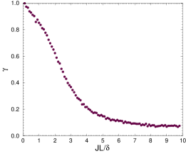
Figure 1: Level statistics parameter $\gamma$ as a function of the coupling parameter $J$ (in units of $\delta/L$), for the model of Eq. (18) for a $3\times 3$ lattice, calculated from the energy levels in the spectral band centered at $-\Delta_{0}$ averaged over 2000 random realizations of $\delta_{i}$ and $J_{i,j}$. The other parameters are $\Delta_{0}=1$ and $\delta=0.09$.

Here we focus on the case $\delta,J\ll\Delta_{0}$, which corresponds to the situation where fluctuations induced by lattice imperfections are relatively weak. In this case, the unperturbed energy spectrum ($J_{i,j}=0$) of Hamiltonian (18) is composed by $L+1$ well separated bands, with inter-band spacing $2\Delta_{0}$. Each band corresponds to states with a given number of spins “up” and spins “down”. The highest density of states is obtained for the central energy band and therefore we expect that quantum chaos shows up first there. When interaction is turned on, a transition to chaos takes place. A value for the chaos border $J_{\mathrm{c}}$ for this transition was given in georgeot00 : $J_{\mathrm{c}}\propto\delta/L$. This border was corroborated in benenti01 , where the emergence of Fermi-Dirac thermalization in the chaotic regime was studied. A careful and detailed analysis of the transition to chaos for this model and its dependence on the size of the lattice has been taken in georgeot00 ; benenti01 . For the sake of comparison with the behavior of the entanglement measures we repeat some of these previous results. We consider a square $3\times 3$ lattice. We note that for lattices composed of an odd number of qubits there is not a central energy band but instead, two central bands centered at $\pm\Delta_{0}$. In what follows, we will consider the states from the central band centered at $-\Delta_{0}$.

We have numerically diagonalized Hamiltonian (18) for different values of the interaction strength. To study the transition to chaos we have obtained the spectral statistics in terms of the nearest neighbor spacing distribution $P(s)$ as well as the structure of the eigenfunctions in terms of the participation number $\xi$. We have restricted our calculations to the energies and eigenstates encountered in the central negative band. For weak interactions the energy domain of this band is clearly visible and we keep the same domain even for stronger interaction where the band structure disappears.

In Fig. 1 the parameter $\gamma$ as a function of the interaction strength is shown for $\Delta_{0}=1$ and $\delta=0.09$. When the strength of the interaction $J$ increases the $P(s)$ distribution smoothly changes from Poisson ($\gamma=1$) towards GOE ($\gamma=0$). Thus, increasing the interaction between the qubits a transition to quantum chaos occurs. In Fig. 1 we observe that the crossover from integrability to chaos takes place in the interval between $JL/\delta\approx 1$ and $JL/\delta\approx 5$.

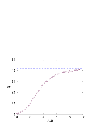
Figure 2: Participation number $\xi$ as a function of $JL/\delta$ for the model of Eq. 18) for a $3\times 3$ lattice, with parameter values as in Fig. 1. The PN was obtained from the central eigenfunction of the band centered at $-\Delta_{0}$ averaged over 2000 random realizations. The dashed line corresponds to $N_{b}/3$.

At the same time, the eigenfunctions start to mix. For weak interactions the eigenfunctions are strongly localized: The number of components in the basis of the unperturbed Hamiltonian is of the order of one. At strong interactions ($JL/\delta\gg 1$) the eigenfunctions are extended, having a large number of non negligible components. This mixing of the eigenfunctions is shown in Fig. 2 in terms of the PN for the same parameter values as in Fig. 1. In Fig. 2 we see that the PN smoothly changes from $1$ (localized regime) to its upper bound value of $N_{b}/3$ (chaotic regime), where $N_{b}$ corresponds to the number of eigenfunctions with energies in the central negative band. As we have discussed, the factor of $1/3$ arises due to the symmetries of the chaotic Hamiltonian that are described by the GOE.

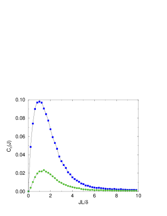
Figure 3: Concurrence $C_{n}$ as a function of the coupling parameter $JL/\delta$ for the model of Eq. (18) for a $3\times 3$ lattice, with parameter values as in Fig. 1. $C_{n}$ was obtained from the central eigenfunction of the central negative band of the spectrum and averaged over all possible pairs of: $a$) nearest neighbors qubits ($n=1$) and $b$) next to nearest neighbors qubits ($n=2$).

We now turn our attention to the entanglement measures. We have calculated the concurrence between nearest ($C_{1}$) and next to nearest ($C_{2}$) neighbor qubits. For this purpose we have drawn $2000$ random realizations of $\delta_{i}$ and $J_{i,j}$ and diagonalized Hamiltonian (18). Using for each realization only the central eigenfunction of the central negative band we have calculated the mean concurrence averaged over all possible nearest neighbor pairs of qubits. In Fig. 3 we show $C_{1}$ (squares) and $C_{2}$ (circles), averaged over all the random realizations as a function of the strength of the interaction. In the basis of the unperturbed Hamiltonian the concurrence is strictly zero. For very weak interactions ($JL/\delta\ll 1$), the concurrence remains small. At the other extreme, when the interaction is very strong ($JL/\delta\gg 1$) and quantum chaos has set in, the concurrence is also small, as expected. Quite interestingly, the maximum of the $C_{1}$ concurrence is for $JL/\delta\approx 1$, that is, in the region in which the crossover from integrability to quantum chaos takes place. In Fig. 3 we can also compare the behavior of $C_{1}$ with that of $C_{2}$. The concurrence of next to nearest neighbor qubits is noticeable smaller than that of nearest neighbor qubits. This is not surprising as the Ising interaction in Eq. (18) couples only nearest neighbor qubits. Therefore, one should expect that quantum correlations between qubits are stronger for qubits that are close than for those farther away. However, we find that $C_{2}$ is not negligible everywhere over the domain of $J$ investigated, except for the integrable and chaotic extremes, where also $C_{1}$ goes to zero. Similarly to $C_{1}$, the concurrence $C_{2}$ has its maximum value for $JL/\delta\approx 1$. It is interesting to point out that, similarly to what happens in the QPT in the Ising model fazio02 ; osborne02 , the concurrences $C_{1}$ and $C_{2}$ exhibit their maximum values close to the value at which quantum chaos sets in. However, besides this similarity, there are other aspects in which the entanglement at the onset of chaos behaves in a different manner than for the case of a QPT. In section IV.2, the qualitative differences of the behavior of entanglement in a QPT an for the onset of quantum chaos that we observe will be discussed.

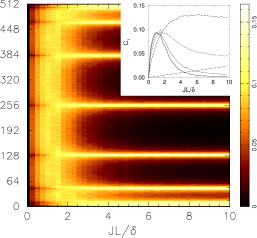
Figure 4: Color density map for the concurrence $C_{1}$ calculated for each individual eigenfunction (index in the vertical axis), averaged over 200 random realizations. $C_{1}$is plotted as a function of the coupling parameter $JL/\delta$ for the model of Eq. (18) for a $3\times 3$ lattice, with parameter values as in Fig. 1. In the inset, we show $C_{1}$ averaged over the central $1/3$ of the eigenstates of each individual band. The different curves correspond to the bands for states with: $4$ (solid), $3$ (dotted), $2$ (dashed), $1$ (long-dashed) and $0$ (dot-dashed) spins “up”.

As we have discussed in section III, the onset of quantum chaos occurs when the typical interaction matrix elements between directly coupled states becomes of the order of their mean level spacing. Thus, the onset of quantum chaos is expected to be observed first at the spectral energies at which the density of directly coupled states is larger. For the models discussed in this and next sections this happens at the center of the spectrum, i.e., in the central bands. Consequently, we focus our discussion on the eigenstates corresponding to the central energy bands. It is worthwhile mentioning that our choice is different from the studies of QPT for which the transition is a property of the ground state. For the case of a transition to quantum chaos we show in Fig. 4 the value of $C_{1}$ as a function of the coupling parameter $J$, calculated for each eigenstates of a $3\times 3$ lattice. The band structure can be clearly seen in the behavior of the concurrence. Inside each band, the concurrence grows from zero at $J\sim 0$ to a maximum close to $JL/\delta=1$, after which it decays again to zero as $J$ is further increased. On the other hand, for the states at the border of the bands, including the ground and the most energetic states, $C_{1}$ behaves quite differently. This is due to the fact that these states do not mix significantly with the other states, as confirmed by our numerical data computing the participation number (data not shown). In the inset of Fig. 4, we show $C_{1}$, averaged over the central eigenstates of each band. We observe that, for all bands, $C_{1}$ reaches its maximum value for $J$ close to $\delta/L$. The fact that for the bands farther away from the center of the spectrum $C_{1}$ decays slower to zero as $J$ is increased is a finite size effect that should disappear at the thermodynamic limit. However, for the ground state $C_{1}$ grows linearly. While we do not discard that at the thermodynamic limit even the concurrence calculated from the ground state will behave in a similar fashion as for any other typical state, Fig. 4 clearly indicates that for a finite system this is not the case.

IV.2 One-dimensional spin chain

In this section we discuss the behavior of bipartite and pairwise entanglement in a family of one-dimensional spin $1/2$ chains. Due to its lower dimensionality these models will allow us to characterize the behavior of the entanglement across the transition to chaos in a deeper fashion than for the previous model. We shall find the same behavior for the concurrence than before. Nevertheless, with these models we are able to analyze its dependence on: the distance in the lattice between the partners, the range of the interaction and the size of the chain. Moreover, for one member of this family of models the chaos border does not coincide with the delocalization border. This will give us the possibility to compare the behavior of the concurrence in a regime of weak and of hard chaos.

IV.2.1 Definition of the model.

We consider a system consisting on a linear chain of $L$ $1/2$ interacting spins, subjected to a static transverse magnetic field (along $z$) and to a circularly polarized magnetic field rotating in the $(x,y)$ plane with frequency $\nu$, ${\vec{B}}(t)=(B^{\perp}\cos(\nu t+\varphi),-B^{\perp}\sin(\nu t+\varphi),B^{z})$ berman01 . In the coordinate system, which rotates around the $z$ axis with frequency $\nu$, the Hamiltonian of this system can be written as

$$\begin{array}[]{ll}H=&-\frac{1}{2}\sum\limits_{k=1}^{L}\{\delta_{k}\sigma^{z}_{k}+\Omega(\cos\varphi~{}\sigma^{x}_{k}-\sin\varphi~{}\sigma^{y}_{k})\}\\ &+\frac{1}{2}\sum\limits_{k=1}^{L-1}J_{k,k+1}\sigma^{z}_{k}\sigma^{z}_{k+1},\end{array}$$ (19)

$\delta_{k}=\omega_{k}-\nu$ where $\omega_{k}$ is the frequency of the precession of the $k$-th spin in the $B^{z}$ field. $\Omega$ stands for the Rabi frequency corresponding to the rotating field and $J_{k,k+1}$ denotes the strength of the Ising interaction between the spins $k$ and $k+1$. The operators $\sigma_{k}$ are the standard Pauli operators acting on the $k$-th spin. In the following, we will take for simplicity $\varphi=\pi/2$ and consider that the static field $B^{z}$ has a constant gradient $a$ along the chain such that $\delta_{k}=ak$. Thus, the Hamiltonian takes the form

$$H=\frac{1}{2}\sum_{k=1}^{L}\left(-\delta_{k}\sigma_{k}^{z}+\Omega\sigma_{k}^{y}\right)-\frac{1}{2}\sum_{k=1}^{L-1}J_{k,k+1}\sigma_{k}^{z}\sigma_{k+1}^{z}\ .$$ (20)

We assume that for all $k$ the inequality $\Omega\gg\delta_{k}$ holds. Open boundary conditions are taken. In berman01 , this model was proposed as a possible candidate for experimental realization of quantum computation. The gradient of magnetic field provides a labeling of qubits in terms of their Larmor frequencies. Thus, it allows for a way to address each qubit separately.

It is worthwhile mentioning that, besides the different dimensionality, there is a more striking difference between this and the previous model: The existence of a constant gradient in the magnetic field gives rise to a $L$-independent threshold for the onset of (weak) chaos. In berman01 the transition to quantum chaos and its implications to quantum computation were explored. Here we want to discuss the behavior of entanglement in this model.

In order to apply the approach discussed in section III it is convenient to represent Hamiltonian (20) in the basis in which it is diagonal for non-interacting spins. In this so-called effective field representation, the one-body unperturbed Hamiltonian $H_{0}$ takes the form

$$H_{0}=\frac{1}{2}\sum_{k=1}^{L}\sqrt{\delta_{k}^{2}+\Omega^{2}}\ \sigma_{k}^{z}$$ (21)

and the interaction Hamiltonian $V$ can be written as $V=V_{\sf diag}+V_{\sf band}+V_{\sf off}$, where

$$V_{\sf diag} = -\frac{1}{2}\sum_{k=1}^{L-1}J_{k,k+1}b_{k}b_{k+1}\sigma_{k}^{z}\sigma_{k+1}^{z},$$

$$V_{\sf band} = -\frac{1}{2}\sum_{k=1}^{L-1}J_{k,k+1}a_{k}a_{k+1}\sigma_{k}^{y}\sigma_{k+1}^{y},$$ (22)

$$V_{\sf off} = \frac{1}{2}\sum_{k=1}^{L-1}J_{k,k+1}\left(a_{k}b_{k+1}\sigma_{k}^{y}\sigma_{k+1}^{z}+a_{k+1}b_{k}\sigma_{k}^{z}\sigma_{k+1}^{y}\right),$$

with

$$a_{k}=\frac{\Omega}{\sqrt{\delta_{k}^{2}+\Omega^{2}}}\quad,\quad b_{k}=\frac{-\delta_{k}}{\sqrt{\delta_{k}^{2}+\Omega^{2}}}\ .$$ (23)

As before, the quantities $J_{k,k+1}$ stand for the Ising interactions between nearest neighbor spins. In what follows, we will consider the interactions to be completely random, i.e. $J_{k,k+1}=J\xi$, where $\xi$ is a random number uniformly distributed in the interval $[-1,1]$. This model is known as the NN model from its nearest neighbor character.

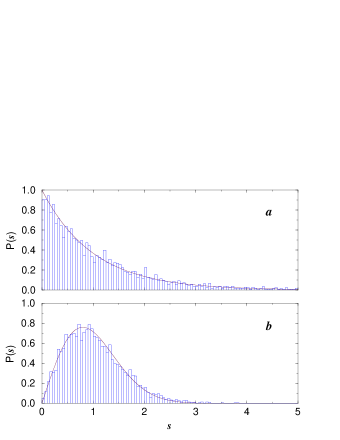
Figure 5: Nearest neighbor level spacing distribution $P(s)$ for the AA model ($l_{c}=L-1$)of Eq. (IV.2.1) for a chain of $12$ qubits and: $a$) $J/J_{\mathrm{c}}=0.35$ and $b$) $J/J_{\mathrm{c}}=15$, calculated from the energy levels in the central band of the spectrum and averaged over 10 random realizations. The solid lines correspond to the Poisson ($a$) and Wigner surmise ($b$) theoretical distributions.

As in the two-dimensional model (18), for the unperturbed ($J=0$) case the spectrum possesses a band structure. Each band is characterized by a constant number $n$ of qubits in the state ${|0\rangle}$ and $L-n$ qubits in the state ${|1\rangle}$. When $L$ is even, a central band (around zero) exists. It consist of the many-qubit states with $L/2$ spins “up” and $L/2$ spins “down”. The number of these states is given by

$$N_{b}=\frac{L!}{\left(L/2\right)!\left(L/2\right)!}\ .$$ (24)

As discussed at the end of previous section, we will only consider the energy levels and energy eigenstates corresponding to the central band of the spectrum.

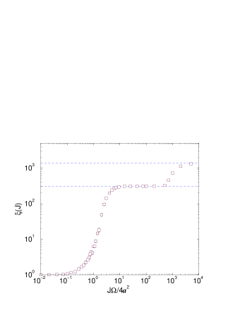
Figure 6: Participation number $\xi$ as a function of the coupling parameter $J$ for the AA model of Eq. (IV.2.1), for a chain of size $L=12$. The PN is averaged over all eigenfunctions in the central band of the spectrum and over 10 random realizations. The dashed horizontal lines correspond to $N_{b}/3$ and to $N/3$ where $N=2^{L}$ is the dimension of the Hilbert space.

When $J>0$ the potential term $V$ mixes the states inside each band and among different bands: In the basis of $H_{0}$, $V_{\sf diag}$ is diagonal. Instead, $V_{\sf band}$ couples states which are either in the same band or in next to nearest bands. $V_{\sf off}$ couples states which are in nearest neighbor bands. The mixing of energy bands triggers the transition to chaos. For a relatively weak interaction the eigenstates (in the basis of $H_{0}$) are localized, while for stronger interaction the number of components significantly different from zero increases. The transition from strongly localized to extended states occurs very fast with the increase of the interaction and sets in when the strength of the typical interaction is of the order of the mean level spacing between directly coupled many-body states many-bodies . In berman01 the value for the delocalization border was found to be $J_{\mathrm{c}}\approx 4a^{2}/\Omega$.

However, as it was shown in berman01 , the NN model is peculiar in the following sense: The delocalization border does not coincide with the chaos border. Increasing the strength of the interaction $J$, the system goes from a regular regime to a weak chaos regime where the eigenfunctions are delocalized but the level statistics is not yet described by Random Matrix Theory. If the interaction is further increased the bands overlap and the system enters a regime of strong chaos. This peculiarity is removed if the range of the interaction is larger than nearest neighbor.

Here we will consider a range of the interaction $l_{c}$ from $1$ (for the NN model) up to $L-1$. The interaction term $V$ keeps the same structure as in Eq. (IV.2.1) but the different terms are now

$$V_{\sf diag} = -\frac{1}{2}\sum_{j=1}^{L-1}\ \sum_{k=j+1}^{j+l_{c}\leq L}J_{jk}b_{j}b_{k}\sigma_{j}^{z}\sigma_{k}^{z},$$

$$V_{\sf band} = -\frac{1}{2}\sum_{j=1}^{L-1}\ \sum_{k=j+1}^{j+l_{c}\leq L}J_{jk}a_{j}a_{k}\sigma_{j}^{y}\sigma_{k}^{y},$$ (25)

$$V_{\sf off} = \frac{1}{2}\sum_{j=1}^{L-1}\ \sum_{k=j+1}^{j+l_{c}\leq L}J_{jk}\left(a_{j}b_{k}\sigma_{j}^{y}\sigma_{k}^{z}+a_{k}b_{j}\sigma_{j}^{z}\sigma_{k}^{y}\right)\ .$$

For $l_{c}=L-1$ this model is known as the AA (All to All) model as in this case all qubits are allowed to interact with each others. In contrast with the NN model ($l_{c}=1$), if $l_{c}>1$ the chaos border occurs at the same value $J_{\mathrm{cr}}\approx 4a^{2}/\Omega$ as the delocalization border berman01 .

IV.2.2 The onset of quantum chaos.

In Fig. 5 the nearest level spacing distribution is shown for the AA model for a chain of $12$ qubits. The $P(s)$ distribution was obtained from the energy levels contained in the central band and averaged over $10$ different random realizations. In panel $a$, the case of weak interaction ($J/J_{\mathrm{c}}=0.35$) is shown. It is in good agreement with the Poisson distribution (solid line), as expected in the integrable regime. In contrast, panel $b$ shows the situation corresponding to strong coupling ($J/J_{\mathrm{c}}=15$) in which the $P(s)$ distribution follows the Wigner surmise expected for a chaotic system with GOE statistics. In panel $b$, the level repulsion effect is evident. Thus, when the interaction strength $J>J_{\mathrm{c}}$, the spectral level statistics changes from Poisson to GOE showing that a transition to quantum chaos is happening.

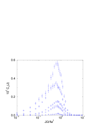
Figure 7: Concurrence as a function of the coupling parameter $J$ for the model of Eq. (IV.2.1) with interaction range $l_{c}=5$ for a chain of $10$ qubits. For each eigenfunction $C_{n}$ was obtained as the average concurrence between all possible pairs of qubits separated by a distance $n$: $n=1$ for nearest neighbors pairs (diamonds), $n=2$ for next to nearest neighbors pairs (right-triangles), $n=3$ (circles), $n=4$ (squares) and $n=5$ (up-triangles). The plotted values correspond to $C_{n}$ averaged over all the eigenstates of the central band and over 30 random realizations.

Simultaneously, a localization-delocalization transition occurs for the eigenstates in the central band. This transition takes place for any value of $l_{c}$. However, for the NN model, the PN does saturate at a value which is lower than $N_{b}/3$ corresponding to the case of Gaussian fluctuations. In Fig. 6, the PN is shown for the AA model for a chain composed of $12$ qubits. The PN (squares) is averaged over all the eigenstates in the central band and over $30$ different random realizations. For weak interactions, the eigenstates are effectively localized ($\xi\approx 1$). The PN increases monotonously with the interaction until it reaches the value $N_{b}/3=308$ (lower dashed line). A complete mixing of different bands occurs for much stronger interactions ($J/J_{\mathrm{c}}\approx 1000$). This is seen in Fig. 6, where $\xi$ increases again and reaches its upper bound value corresponding $N/3$, namely to one third of the dimension of the whole Hilbert space, as expected from RMT.

The model of Eq. (IV.2.1) shows a clear transition to quantum chaos in which both energy levels and eigenstates change their character. Now we turn our attention to the behavior of quantum entanglement.

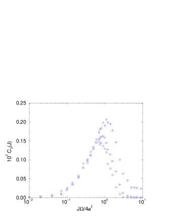
Figure 8: Mean concurrence $C_{3}$ between qubits at a distance $n=3$, averaged over all the eigenfunctions in the central band of the spectrum and over 30 random realizations. The mean concurrence is plotted as a function of the coupling parameter $J$ for the model of Eq. (IV.2.1) in a chain of $10$ qubits. We compare $C_{3}$ for different range of the interaction: The NN model corresponding to $l_{c}=1$ (diamonds), $l_{c}=2$ (triangles), and $l_{c}=3$ (circles).

IV.2.3 The concurrence: Sharing of entanglement.

We have calculated the mean concurrence averaged over all the eigenstates in the central band as a function of the strength $J$ of the interaction. In Fig. 7 the mean concurrence is shown for the model of Eq. (IV.2.1) for a chain of $L=10$ qubits, with an interaction that couples $L/2$ neighbor qubits, i.e., $l_{c}=5$. The diamond symbols correspond to the mean concurrence $C_{1}$ between nearest neighbor qubits . As it was discussed in section III.3, we observe that $C_{1}$ is close to zero in both extremes of chaos and of integrability. Moreover, similarly to what we have observed for the two-dimensional model (18), in between the integrable and the chaotic extremes the concurrence increases and its maximum value is close to the value for the chaos border. Despite the fact that we have observed this behavior of concurrence for just two different models we conjecture that it is generic for transitions to chaos. In Fig. 7 the mean concurrence averaged over all qubits at further distances, $C_{2}$ (right-triangles), $C_{3}$ (circles), $C_{4}$ (squares) and $C_{5}$ (up-triangles) are also shown. The behavior of $C_{1}$ and $C_{2}$ is similar to that observed for the two-dimensional model. We see that the concurrence $C_{n}$ decreases with the distance $n$, except for weak interactions for which $C_{2}>C_{1}$. This latter is a peculiarity of this model. It is interesting to notice that the coupling strength $J_{\rm max}(n)$ at which the concurrence $C_{n}$ takes its maximum value does not change significantly with $n$.

Let us now consider the following question: for a given distance $n$, how does $C_{n}$ varies if the range of the interaction increases? In Fig. 8 the mean concurrence $C_{3}$ is plotted for different ranges $l_{c}$ of the interaction: $l_{c}=1$ (diamonds), $l_{c}=2$ (triangles) and $l_{c}=3$ (circles). To this purpose, we computed $C_{3}$ for all the eigenfunctions in the central band of the spectrum of a chain of size $L=10$ and averaged over $30$ different random realizations. From Fig. 8 we observe that as the range of the interaction increases the mean concurrence $C_{3}$ decreases. The same conclusions were also obtained for the behavior $C_{n}$ with $n\neq 3$ (data not shown). This fact can be understood from the pairwise character of the concurrence. Since the amount of entanglement between one definite qubit and the rest of the system is bounded, this finite amount of entanglement has to be shared between all possible partners. When the range of the interaction is enlarged, it becomes easier for each qubit to become entangled with more qubits in the chain. As a result the pairwise entanglement between one single qubit and the rest of the chain is shared among more partners. Therefore, the average entanglement shared between two qubits decreases. This argument is valid if a change in the range of the interaction does not significantly change the total amount of bipartite entanglement that is shared between a single qubit and the rest of the chain.

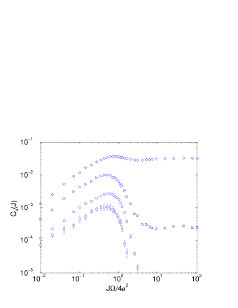
Figure 9: Mean concurrence averaged over all possible pairs of qubits for all the eigenstates in the central band of the spectrum and over 30 random realizations for the AA model of Eq. (IV.2.1) ($l_{c}=L-1$) as a function of the coupling parameter $J$ and for different sizes of the chain of qubits: $L=6$ (diamonds), $L=8$ (triangles), $L=10$ (circles), $L=12$ (squares).

Finally, we have studied the behavior of the concurrence as a function of the size of the system. In Fig. 9 the mean concurrence $C_{a}$ obtained from all possible pairs of qubits is shown for the AA model for different sizes of the chain: $L=6$ (diamonds), $L=8$ (triangles), $L=10$ (circles), $L=12$ (squares). In this case, instead of measuring the concurrence $C_{n}$ for some value of $n$, we have measured the concurrence $C_{a}$ as the mean concurrence between all possible pairs of qubits in the chain. This is because, for the AA model, the concept of distance turns out to be meaningless, since the strength of the interaction between two qubits does not depend on their distance. The behavior of $C_{a}$ as a function of the size of the system can be well understood in terms of the same argument used to explain Fig. 8. When the system size is increased, the number of possible partners with which a given qubit can be entangled also increases. Therefore, the pairwise entanglement decreases, in agreement with the data of Fig. 9. We note that, for small system sizes ($L=6,8$), the concurrence $C_{a}$ does not go to zero at the chaotic side of the transition. This finite-size effect disappears already for $L=10,12$. Similar results were obtained for the other models with different range of the interaction.

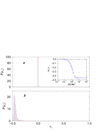
Figure 10: Normalized distribution $P(c_{\lambda})$ of the quantity $c_{\lambda}=\lambda_{1}-\lambda_{2}-\lambda_{3}-\lambda_{4}$ of Eq. (5) for the AA model Eq. (IV.2.1) with $L=12$ and coupling: $a$) $J/J_{\mathrm{c}}=0.01$ and $b$) $J/J_{\mathrm{c}}=100.0$. In the inset the behavior of the first moment of the distribution $<c_{\lambda}>$ is shown as a function of the coupling parameter $J$.

The results presented in this section show that the concurrence maximizes for values of $J$ which are close to those at which the transition to chaos occurs. As discussed in the previous section, the same behavior for the maximum of concurrence has also been observed for quantum phase transitions occurring in integrable models (see, e.g., fazio02 ; osborne02 for a study on the Ising chain). However, as it can be seen in Fig. 8 for the transition to chaos, the concurrence approaches zero when the size of the system increases, in contrast to what is observed in QPT fazio02 , where $C_{n}\rightarrow 0$ for all $n>1$ but remains finite for $n=1$. In these studies a critical scaling for the derivative of the concurrence was obtained. On one hand, the fact that for the onset of quantum chaos the concurrence diminishes when the system approaches the thermodynamic limit makes a finite size scaling analysis rather difficult, as numerical errors become soon of the same order of the measure itself. On the other hand, it is not clear whether the transition to chaos in the models we have considered becomes sharp at the thermodynamic limit. This means that to prove the existence of a critical point for the transition remains an open problem. In order words, we lack for a critical point at which to perform a scaling analysis. We have nevertheless analyzed the dependence of $\mathrm{d}C/\mathrm{d}J$ on the system size without having found any clear indication of a scaling behavior (data not shown).

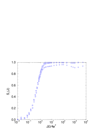
Figure 11: Von Neumann entropy $S_{1}$ between one qubit and the rest of the system; $S_{1}$ is averaged over all qubits and over all eigenstates in the central band of the spectrum and over 30 random realizations for the AA model of Eq. (IV.2.1) as a function of the coupling parameter $J$ and for different sizes of the chain of qubits: $L=6$ (diamonds), $L=8$ (triangles), $L=10$ (circles), $L=12$ (squares).

It is interesting to study the different character of mixed pairwise entanglement in the integrable and chaotic sides of the transition. In Sec. III.3, we gave simple arguments that explain the different structure of the reduced density matrix $\tilde{\rho}$ for a mixed bipartite state in the regimes of integrability and chaos. In the integrable region, due to the localized nature of the eigenstates, $\tilde{\rho}$ is essentially diagonal with only one matrix element significantly different from zero. On the other hand, in the chaotic region, $\tilde{\rho}$ is almost diagonal with matrix elements of comparable magnitude along the diagonal. Both cases give a very small (or zero) concurrence. However, while in the integrable case this is due to the fact that the two-qubit subsystem under investigation is essentially in a separable pure state, in the chaotic case the pairwise entanglement is zero due to the random structure of the eigenfunctions of the whole $L$-spin system. As a consequence, the two-qubit reduced density matrix is essentially diagonal. Therefore, in the chaotic regime, the interaction with the rest of the system mimics a decoherence process for the two-qubit subsystem.

The different origin of the very small value of concurrence is illustrated by the distribution of the $c_{\lambda}$’s (we remind the reader that the concurrence is defined as the maximum between $c_{\lambda}$ and $0$, see Eq. (5)). In Fig. 10, the probability distribution $P(c_{\lambda})$ is shown in: $a$) the integrable regime and $b$) the chaotic regime, for the AA model and a chain of size $L=12$. Clearly, in both cases the probability to find $c_{\lambda}>0$ is very small. Therefore, the concurrence is very small in both cases. However, the distributions $P(c_{\lambda})$ are quite different. We note that numerical results about the distribution $P(c_{\lambda})$ in a different model of quantum chaos where presented in caves . In the Inset of Fig. 10, one can see that the first moment of $P(c_{\lambda})$ changes across the chaos border. It is an interesting open problem to obtain an analytical form of $P(c_{\lambda})$ for integrable and chaotic situations. The possibility to use this distribution to mark the transition to chaos also deserves more investigation.

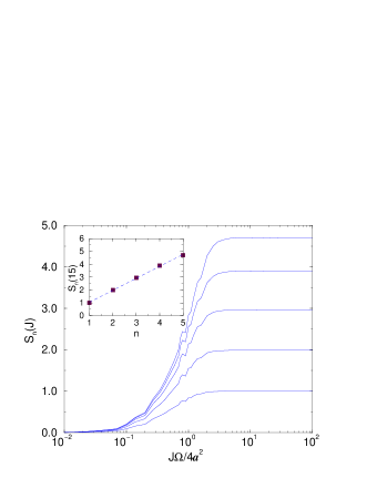
Figure 12: Von Neumann entropy $S_{n}$ between left and right blocks of sizes $n$ and $L-n$ qubits, respectively, averaged over all eigenfunctions in the central band of the spectrum and over 10 random realizations. The data correspond to the AA model of Eq. (IV.2.1) for a chain of size $L=12$. From bottom to top, the different curves are from $n=1$ to $n=5$. In the inset $S_{n}(J/J_{\mathrm{c}}=15)$ is plotted as a function of $n$. The dashed line corresponds to a linear fit with a slope of $0.93\pm 0.02$.

IV.2.4 The Von Neumann entropy.

We now turn our attention to the behavior of bipartite entanglement measured in terms of the Von Neumann entropy. First we consider the mean Von Neumann entropy $S_{1}$ of each qubit with the rest of the qubits in the chain. For this purpose, we divide the system in two parties: one consists of just one qubit and the other contains the remaining $L-1$ qubits. Then, following Eq. (1), we compute $S_{1}$ from the $2\times 2$ reduced density matrix of the one qubit subsystem. In Fig. 11 the behavior of $S_{1}$ across the transition to chaos is shown for the AA model and for different sizes of the system, from $L=6$ to $L=12$. We find that the bipartite entanglement $S_{1}$ shows the same behavior independently of the size of the system. The state of the system changes from separable to maximally entangled as the transition to chaos occurs. In all cases, the entropy saturates to its maximum value $S_{1}=1$, up to corrections of order $1/2^{L}$ random-states . As discussed in Sec. II, these results show that there exists a global entanglement of each single qubit with the rest of the system and that this entanglement increases with the interaction. The maximum value of bipartite entanglement is obtained when quantum chaos has set in.

We have obtained similar results for the bipartite entanglement when the two blocks in which the system is partitioned have different lengths. As an example we show in Fig. 12 the Von Neumann entropy $S_{n}$ between a block of size $n$ and the rest of the system (of size $L-n$) from $n=1$ (bottom) to $n=5$ (top) for the AA model and a chain of size $L=12$. Similarly to the $S_{1}$ case, $S_{n}$ increases when the transition to chaos occurs and saturates to $S_{n}\approx n$ for large interaction strength. Hence, the state of the system becomes maximally entangled when chaos sets in. This is a direct consequence of the existence of multipartite entanglement. Moreover, in the inset of Fig. 12, we have plotted the saturation value of $S_{n}$ for $J/J_{\mathrm{c}}=15$ as a function of the size of subsystems $n$. This shows that in the chaotic regime the bipartite entanglement scales linearly with the size of the smallest of the two blocks in which the global system has been partitioned: $S_{n}\propto n$.

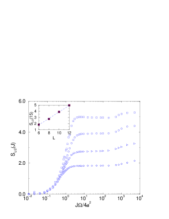
Figure 13: Von Neumann entropy $S_{L/2}$ as a function of the strength of the interaction $J$, averaged over all eigenfunctions in the central band of the spectrum and over 10 random realizations. The data correspond to the AA model of Eq. (IV.2.1) for a chain of sizes $L=6$ (diamonds), $L=8$ (triangles), $L=10$ (circles), $L=12$ (squares). In the inset $S_{L/2}(J/J_{\mathrm{c}}=15)$ is plotted as a function of $L$. The dashed line corresponds to a linear fit with a slope of $0.52\pm 0.02$.

It is interesting to study the Von Neumann entropy as a function of the system size $L$, when the two blocks in which the system is partitioned have a size $\propto L$. We have computed the bipartite entanglement $S_{L/2}$ corresponding to the case in which the system is partitioned in two halves. A value of $S_{L/2}>0$ for any $L$ is indicative of the existence of multipartite entanglement. The obtained behavior of $S_{L/2}$ as a function of the strength of the interaction is shown in Fig. 13, for different system sizes. The behavior of $S_{L/2}$ is similar to that shown by $S_{1}$. It takes very small values in the integrable regime and then increases with the interaction up to a value for which it saturates. The saturation value is $\approx L/2$ (up to corrections of $\mathcal{O}(1)$ random-states ). In the inset of Fig. 13, we plot the value of $S_{L/2}$ for $J/J_{\mathrm{c}}=15$ (i.e., in the chaotic regime in which the eigenstates in the central band are effectively mixed) as a function of the size $L$ of the system. It is interesting to note that the Von Neumann entropy does feel the mixing of different spectral bands occurring for a very strong interaction ($J/J_{\mathrm{c}}\sim 1000$). The inter-band mixing (compare with Fig. 6 for $L=10$) produces a increase in the Von Neumann entropy which nevertheless is small compared to that observed for the onset of chaos. This is in contrast with the pairwise measures such as the concurrence, for which we did not observed any change.

In addition, for any given value of $J$ when chaos has set in, the bipartite entanglement scales linearly with the size of the system. It is interesting to comment this result from the viewpoint of computational complexity. It was shown in vidal that large entanglement of the quantum computer hardware is a necessary condition for exponential speedup (with respect to classical computation) in quantum computation operating on pure states. To be more precise, a necessary condition for an exponential speedup is that the amount of entanglement increases greater than logarithmically with the size $L$ of the computation. This condition is fulfilled in the chaotic regime where $S_{L/2}\propto(L/2)$. We remark that, differently from problems like exact cover Orus , this is not limited to the transition region but extends to the whole chaotic regime. We also note that the relation between entanglement and computational complexity in quantum algorithms simulating quantum chaos has been investigated in Ref. montangero .

IV.3 Weak and hard chaos

In this section, we discuss the behavior of quantum entanglement in situations of weak and of hard chaos. As it was discussed, the NN model of Eq. (IV.2.1), while similar in character to the model of Eq. (IV.2.1) with $l_{c}>1$, shows a quite unexpected peculiarity: The chaos border does not coincide with the delocalization border. Thus, when the strength of the interaction is increased, the NN model experiences a transition from integrability to a situation of weak chaos in which the eigenfunctions are delocalized while the level statistics is yet of Poissonian nature. This results from the fact that the NN Hamiltonian can be approximately mapped into a model of $L$ free fermions as discussed in free-fermions . However, this non generic situation is removed if longer ranges of the interaction are considered. This gives us the possibility to compare the behavior of entanglement in situations of weak and hard chaos.

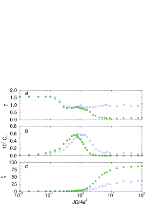
Figure 14: Comparison between the NN model Eq. (IV.2.1) (circles) and the model of Eq. (IV.2.1) with $l_{c}=L/2$ (squares), for a chain of qubits of length $L=10$. ¿From top to bottom, the three panels show, as a function of the coupling parameter $J$: the behavior of the spectral statistics parameter $\gamma$ (top panel); the mean concurrence $C_{1}$ between nearest neighbor pairs of qubits (middle panel); the participation number $\xi$ (bottom panel). All quantities were calculated in the central band of the spectrum and averaged over 30 random realizations.

We have calculated the nearest neighbor concurrence $C_{1}$ for the NN model and for a long range interaction model with $l_{c}=L/2$. In Fig. 14 we present our results. In panels ($a$) and ($c$) the $\gamma$ parameter and the PN $\xi$ are shown, respectively. We can clearly see the peculiar behavior of the NN model. For both NN (open circles) and $l_{c}=L/2$ (solid squares) models the PN behaves in a similar way. For the NN model the PN signals a clear transition from localized to delocalized eigenstates, even thought it does not saturates at the value corresponding to Gaussian fluctuations. In particular, the delocalization border of both models coincide. Nevertheless, the $\gamma$ parameter shows a very different behavior. For interaction strengths $0.2\leq J/J_{\mathrm{c}}\leq 1$ the level statistics parameter $\gamma$ for both models takes the value $\gamma\approx 1$. This corresponds to the integrable case in which the nearest neighbor spacing distribution is Poissonian. However, for the NN model, $\gamma$ remains Poissonian for larger values of the interaction up to $J/J_{\mathrm{c}}\approx 100$. This is the situation that has been termed as weak chaos. In contrast, for the $l_{c}=L/2$ model the level statistics changes from Poissonian ($\gamma=1$), to GOE ($\gamma=0$), around $J/J_{\mathrm{c}}=1$. Thus, for the $l_{c}=L/2$ model the chaos border coincides with the delocalization border as it is commonly found in many-particle systems with two-body interaction.

In panel ($b$) the corresponding results for the concurrence $C_{1}$ are shown. We observe again the difference in $C_{1}$ due to the range of the interaction, as discussed in the previous subsection. Despite this difference, $C_{1}$ shows a similar behavior for both models: It is small at both sides of the transition and increases in between, having its maximum value close to $J/J_{\mathrm{c}}=1$. This numerical results suggest that the behavior of the pairwise entanglement is more sensitive to the mixing of the eigenstates than to the onset of quantum chaos.

V Final Remarks

We have studied the bipartite and pairwise entanglement in one and two dimensional spin lattice models that experience a transition to quantum chaos.

To study the presence of multipartite entanglement, we have analyzed the behavior of the averaged Von Neumann entropy for subsystems of different sizes. In particular, we have shown that, for a partition of the system into two equal-size subsystems, this quantity grows linearly with the system size in the chaotic regime. This shows that the classical simulation method discussed in vidal cannot be used to efficiently simulate the quantum chaos regime on a classical computer.

For the case of pairwise entanglement, we have studied the dependence of the concurrence on the distance between the partners, the range of the interaction and the size of the system. Our results suggest that for a typical many-qubit state, the entanglement is mainly multipartite rather than pairwise.

We have also discussed the different character that the pairwise entanglement has at the integrable and the chaotic side of the transition in terms of a suitable distribution of the eigenvalues of the two-spin reduced density matrix. The use of the moments of this distribution to mark the transition to quantum chaos remains and interesting open question.

Finally, we have discussed the similarities and differences between the behavior of the concurrence at a quantum phase transition and at the onset of quantum chaos. Our results show that the maximal concurrence is obtained close to the delocalization border for which mixing of the noninteracting eigenfunctions takes place and not necessarily related to the onset of quantum chaos.

This work was supported in part by the EC contract IST-FET EDIQIP, the NSA and ARDA under ARO contract No. DAAD19-02-1-0086, and the PRIN 2002 “Fault tolerance, control and stability in quantum information processing”. We acknowledge useful discussions with B. Georgeot, F. Izrailev, D. Shepelyansky, T.H. Seligman, and V. Sokolov. C.M.-M. acknowledges the hospitality of “Centro Internacional de Ciencias” where part of this work has been done.

References

- (1) M.A. Nielsen and I.L. Chuang, Quantum Computation and Quantum Information (Cambridge University Press, Cambridge, 2000).
- (2) G. Benenti, G. Casati, and G. Strini, Principles of Quantum Computation and Information, Vol. I: Basic concepts (World Scientific, Singapore, 2004).
- (3) R. Jozsa and N. Linden, Proc. R. Soc. Lond. A 459, 2011 (2003).
- (4) C. Miquel, J.P. Paz, and R. Perazzo, Phys. Rev. A 54, 2605 (1996).
- (5) C. Miquel, J.P. Paz, and W.H. Zurek, Phys. Rev. Lett. 78, 3971 (1997).
- (6) P.H. Song and D.L. Shepelyansky, Phys. Rev. Lett. 86, 2162 (2001).
- (7) G.G. Carlo, G. Benenti, and G. Casati, Phys. Rev. Lett. Phys. Rev. Lett. 91, 257903 (2003); G.G. Carlo, G. Benenti, G. Casati, and C. Mejía-Monasterio, Phys. Rev. A 69, 062317 (2004).
- (8) D. Rossini, G. Benenti, and G. Casati, Phys. Rev. A 69, 052317 (2004).
- (9) P. Facchi, S. Montangero, R. Fazio, and S. Pascazio, quant-ph/0407098.
- (10) B. Georgeot and D.L. Shepelyansky, Phys. Rev. E 62, 3504 (2000); ibid. 62, 6366 (2000).
- (11) V.V. Flambaum, Aust. J. Phys. 53, 489 (2000).
- (12) G. Benenti, G. Casati, and D.L. Shepelyansky, Eur. Phys. J. D 17, 265 (2001).
- (13) G.P. Berman, F. Borgonovi, F.M. Izrailev, and V.I. Tsifrinovich, Phys. Rev. E 64, 056226 (2001); ibid. 65, 015204(R) (2001).
- (14) V. Zelevinsky, B.A. Brown, N. Frazier and M. Horoi Phys. Rep. 276, 85 (1996); V.K.B. Kota, Phys. Rep. 347, 223 (2001); L. Benet and H.A. Weidenmüller J. Phys. A: Math. Gen. 36, 3569 (2003)
- (15) G. Montambaux, D. Poilblanc, J. Bellissard and C. Sire, Phys. Rev. Lett., 70, 497 (1993); D. Poilblanc, T. Ziman, J. Bellissard, F. Mila and G. Montambaux, Europhys. Lett., 22, 537 (1993); T.C. Hsu and J.C. Anglès d’Auriac, Phys. Rev. B., 47, 14291 (1993); Y. Avishai, J. Richert and R. Berkovits, Phys. Rev. B., 66, 052416 (2002); J.Ch. Anglès d’Auriac and J.-M. Maillard, Physica A, 321, 325 (2003);
- (16) F.M. Izrailev, in varena99 , p. 371, and references therein.
- (17) P.A. Lee and T.V. Ramakrishnan, Rev. Mod. Phys. 57, 287 (1985); U. Sivan and Y. Imry, Phys. Rev. B 35 6074 (1987); B.I. Shklovskii, B. Shapiro, B.R. Sears, P. Lambrianides and H.B. Shore, Phys. Rev. B 47 11487 (1993); I. K. Zharekeshev and B. Kramer,Phys. Rev. B 51 R17239 (1995).
- (18) S. Sachdev, Quantum Phase Transitions (Cambridge University Press, Cambridge, 1999).
- (19) T.J. Osborne and M.A. Nielsen, Quantum Information Processing 1, 45 (2002).
- (20) A. Volya and V. Zelevinsky, Phys.Lett. B574, 27 (2003).
- (21) A. Osterloh, L. Amico, G. Falci, and R. Fazio, Nature 416, 609 (2002); L. Amico, A. Osterloh, F. Plastina, R. Fazio, and G.M. Palma, Phys. Rev. A 69, 022304 (2004).
- (22) T.J. Osborne and M.A. Nielsen, Phys. Rev. A 66, 032110 (2002).
- (23) I. Bose and E. Chattopadhyay, Phys. Rev. A 66, 062320 (2002).
- (24) G. Vidal, J.I. Latorre, E. Rico, and A. Kitaev, Phys. Rev. Lett. 90, 227902 (2003).
- (25) S.J. Gu, H.Q. Lin, and Y.Q. Li, Phys. Rev. A 68, 042330 (2003).
- (26) U. Glaser, H. Büttner, and H. Fehske, Phys. Rev. A 68, 032318 (2003).
- (27) V.E. Korepin, Phys. Rev. Lett. 92, 096402 (2004).
- (28) J. Vidal, G. Palacios, and R. Mosseri, Phys. Rev. A 69, 022107 (2004); J. Vidal, R. Mosseri, and J. Dukelsky ibid. 69, 054101 (2004).
- (29) F. Verstraete, M. Popp, and J.I. Cirac, Phys. Rev. Lett. 92, 027901 (2004).
- (30) J.I. Latorre, R. Orús, E. Rico and J. Vidal, cond-mat/0409611.
- (31) S. Montangero, G. Benenti, and R. Fazio, Phys. Rev. Lett. 91, 187901 (2003).
- (32) L.F. Santos, G. Rigolin, and C.O.Escobar, Phys. Rev. A 69, 042304 (2004).
- (33) N. Lambert, C. Emary, and T. Brandes, Phys. Rev. Lett. 92, 073602 (2004).
- (34) S. Bettelli and D.L. Shepelyansky, Phys. Rev. A 67, 054303 (2003).
- (35) A.J. Scott and C.M. Caves, J. Phys. A 36, 9553 (2003).
- (36) A. Lahiri, quant-ph/0302029.
- (37) X. Wang, S. Ghose, B.C. Sanders, and B. Hu, quant-ph/0312047.
- (38) W.K. Wootters, Quantum Inf. and Comp. 1, 27 (2001).
- (39) C.H. Bennett, D.P. DiVincenzo, J.A. Smolin, and W.K. Wootters, Phys. Rev. A 54, 3824 (1996).
- (40) W.K. Wootters, Phys. Rev. Lett. 80, 2245 (1998).
- (41) C.H. Bennett, G. Brassard, S. Popescu, B. Schumacher, J.A. Smolin, and W.K. Wootters, Phys. Rev. Lett. 76, 722 (1996).
- (42) K. Zyczkowski, P. Horodecki, A. Sanpera, and M. Lewenstein, Phys. Rev. A 58, 883 (1998); G. Vidal and R.F. Werner, ibid. 65, 032314 (2002).
- (43) V. Vedral, M.B. Plenio, K. Jacobs, and P.L. Knight, Phys. Rev. A 56, 4452 (1997).
- (44) D. Bruß, J. Math. Phys. 43, 4237 (2002).
- (45) E.P. Wigner, Ann. Phys. (N.Y.) 53, 36 (1951); ibid. 62, 548 (1955); ibid. 67, 325 (1958); F.J. Dyson, J. Math. Phys. 3, 140 (1962); M.L. Mehta, Random Matrices and the Statistical Theory of Energy Levels (Academic Press, New York, 1967);
- (46) T.A. Brody, J. Flores, J.B. French, P.A. Mello, A. Pandey, and S.S.M. Wong, Rev. Mod. Phys. 53, 385 (1981).
- (47) T. Guhr, A. Müller-Groeling, and H.A. Weidenmüller, Phys. Rep. 299, 189 (1998).
- (48) New Directions in Quantum Chaos, Proceedings of the International School of Physics “Enrico Fermi”, Course CXLIII, Varena (1999), eds. G. Casati, I. Guarneri, and U. Smilansky (IOS Press, Amsterdam, 2000).
- (49) F. Haake, Quantum Signatures of Chaos (2nd. Ed.), (Springer-Verlag, Berlin, 2000).
- (50) O. Bohigas, M.-J. Giannoni, and C. Schmit, Phys. Rev. Lett. 52, 1 (1984).
- (51) G. Casati, F. Valz-Gris, and I. Guarneri, Lett. Nuovo Cimento 28, 279 (1980).
- (52) L. Benet, T.H. Seligman, and H.A. Weidenmüller, Phys. Rev. Lett. 71, 529 (1993).
- (53) D.N. Page, Phys. Rev. Lett. 71, 1291 (1993); S.K. Foong, S. Kanno ibid. 72, 1148 (1993); S. Sen ibid. 77, 1 (1996).
- (54) E. Lieb, T. Schultz, and D. Mattis, Ann. Phys. (N.Y.) 16, 407 (1961); A.P. Young and H. Rieger, Phys. Rev. B 53, 8486 (1997).
- (55) G. Vidal, Phys. Rev. Lett. 91, 147902 (2003).
- (56) R. Orús and J.I. Latorre, Phys. Rev. A 69, 052308 (2004).
- (57) S. Montangero, Phys. Rev. A 70, 032311 (2004).