Matter diffraction at oblique incidence: Higher resolution and the ⁴He₃ Efimov state

Abstract

We study the diffraction of atoms and weakly-bound three-atomic molecules from a transmission grating at non-normal incidence. Due to the thickness of the grating bars the slits are partially shadowed. Therefore, the projected slit width decreases more strongly with the angle of incidence than the projected period, increasing, in principle, the experimental resolution. The shadowing, however, requires a revision of the theory of atom diffraction. We derive an expression in the style of the Kirchhoff integral of optics and show that the diffraction pattern exhibits a characteristic asymmetry which must be accounted for when comparing with experimental data. We then analyze the diffraction of weakly bound trimers and show that their finite size manifests itself in a further reduction of the slit width by $(3/4)\left\langle r\right\rangle$ where $\left\langle r\right\rangle$ is the average bond length. The improved resolution at non-normal incidence may in particular allow to discern, by means of their bond lengths, between the small ground state of the helium trimer ($\left\langle r\right\rangle\approx 1\,$nm, Barletta and Kievsky, Phys. Rev. A 64, 042514 (2001)) and its predicted Efimov-type excited state ($\left\langle r\right\rangle\approx 8\,$nm, ibid.), and in this way to experimentally prove the existence of this long-sought Efimov state.

I Introduction

The combination of two unique features makes matter-wave diffraction of noble gas trimers an outstanding enterprise. Firstly, diffraction presently is the only experimental technique which allows to detect such very weakly bound clusters and to determine their properties Luo et al. (1995); Schöllkopf and Toennies (1994); Grisenti et al. (2000a). Secondly, the helium trimer ⁴He₃ is the only molecule predicted to possess an Efimov-type bound state Lim et al. (1977); Esry et al. (1996); Barletta and Kievsky (2001) under normal conditions footnote-ultracold .

Only recently did diffraction of atomic and molecular beams evolve towards a precise experimental technique. Early pioneering experiments had proved diffraction for a sodium beam through a grating initially fabricated for x-rays Keith et al. (1988), as well as for meta-stable helium Carnal and Mlynek (1991) and for neon Shimizu et al. (1992) through micrometer double-slits. Later, transmission gratings with a period of $d=200$ nm had brought an improvement, but finally the production of reliable nano-scale transmission gratings with a period of only $d=100$ nm Savas et al. (1995) paved the way for quantitative matter diffraction experiments with an unparalleled spatial coherence across up to a hundred slits for a helium atom beam Grisenti et al. (1999). Unprecedented, matter diffraction also allows to investigate the coherence properties of very heavy molecules with many internal degrees of freedom such as fullerenes Arndt et al. (1999); Hornberger et al. (2003).

Classical wave optics can merely serve as an approximation to the underlying physical scattering process of atom diffraction. The hierarchy of the diffraction peak intensities in a diffraction experiment with neutral atoms or molecules is significantly affected by the weak van der Waals surface force, which acts on atoms in the vicinity of the material grating. This was included in a quantitative theory in Refs. Hegerfeldt and Köhler (1998); Hegerfeldt and Köhler (2000a) which allowed, in comparison with experimental data, to characterize this surface force for the noble gases helium, neon, argon, and krypton, and the covalently bound D₂ molecule Grisenti et al. (1999), as well as for meta-stable helium and neon Brühl et al. (2002).

Moreover, there is no analog in wave optics for the diffraction of weakly bound small noble gas van der Waals clusters such as the helium dimer ⁴He₂ and trimer ⁴He₃. Experimental evidence for these delicate molecules was for the first time unambiguously provided through the mass-selective property of grating diffraction Schöllkopf and Toennies (1994). Moreover, the comparatively large interatomic distance of $\left\langle r\right\rangle=5.2$ nm in ⁴He₂, implied by the small binding energy $E_{\text{b}}=-1.1$ mK Grisenti et al. (2000a), was shown to manifest itself as an apparent narrowing of the grating slits by $\frac{1}{2}\left\langle r\right\rangle$. It was this size effect which rendered possible the determination of $\left\langle r\right\rangle$ from experimental diffraction data Grisenti et al. (2000a). This allowed for comparison with modern realistic helium-helium potentials of Refs. Janzen and Aziz (1995); Gdanitz (2001).

Numerical studies of the helium trimer relying on these helium-helium potentials Lim et al. (1977); Huber and Lim (1977); Nakaichi-Maeda and Lim (1983); Fedorov and Jensen (1993); Nielsen et al. (1998); Motovilov et al. (1997); Kolganova et al. (1998); Roudnev and Yakovlev (2000); Motovilov et al. (2001); Esry et al. (1996); Bruch (1999); Barletta and Kievsky (2001), quantum Monte Carlo simulations Lewerenz (1997), as well as quantum chemical ab initio calculations Røeggen and Almlöf (1995) have long predicted two bound states for ⁴He₃: a ground state at $-126$ mK and a shallow excited state at $-2.3$ mK Barletta and Kievsky (2001). Moreover, the excited state is believed to be an Efimov-type state. Originally in the context of nuclear physics, Efimov Efimov (1970) had shown that if the scattering length of a pair potential exceeds the effective range of the potential by far then a universal series of bound states exists in the three-body system near the dissociation threshold. Examples for such Efimov states, however, have been searched for in vain in three-nucleon systems, leaving the three-atomic helium molecule presently as the only candidate.

The ⁴He₃ excited state cannot experimentally be distinguished from the ground state by its mass. However, due to the large difference in binding energy, both predicted states have markedly different interatomic distances: $\left\langle r\right\rangle=0.96$ nm in the ground state and $\left\langle r\right\rangle=7.97$ nm in the excited state Barletta and Kievsky (2001). Therefore, the size effect, which had previously played the essential role in the dimer diffraction experiment and which we show to be $\frac{3}{4}\left\langle r\right\rangle$ for a trimer, is expected to render the two states distinguishable. Bruch et al have analyzed the mole fraction of small helium clusters (including atoms) in a nozzle beam diffraction setup and showed that up to 7% can be trimers Bruch et al. (2002). This should be an ample amount for a quantitative analysis. The population ratio of ground state vs. excited state trimers in the beam is, however, not known. It is therefore essential to provide sufficient experimental resolution for the small ground state in order to evaluate diffraction data from a mixed beam. A limitation in the resolution is posed by the period of the grating, $d=100\,$nm, and the slit width, typically $s_{0}=60$ nm, which are both large compared to the ground state size. Transmission gratings with smaller periods and slit widths are, however, presently not available.

To address this issue we consider diffraction from a custom transmission grating at oblique (non-normal) incidence, i.e. the grating is rotated by an angle $\theta^{\prime}$ about an axis parallel to its bars. The grating typically consists of a $t\approx 120$ nm thick layer of silicon nitride into which the slits have been etched in a lithographic production process Savas et al. (1995). As the grating is rotated the upstream edges of its bars cut into the incident beam, partially shadowing the slits. By this effect the projected slit $s_{\perp}$ width (perpendicular to the incident beam) decreases more strongly with $\theta^{\prime}$ than the projected period $d_{\perp}$. Since the diffraction pattern is roughly governed by the squared slit function Born and Wolf (1959)

$$\left[\frac{\sin(n\pi s_{\perp}/d_{\perp})}{(n\pi s_{\perp}/d_{\perp})}\right]^{2}$$

where $n$ denotes the diffraction order, one expects that at non-normal incidence more atoms or molecules are diffracted into higher diffraction orders. For example, at $t=120\,$nm and an angle of incidence (rotation angle) of $\theta^{\prime}=21^{\circ}$ the ratio $d_{\perp}/s_{\perp}$ is twice as large as $d/s_{0}$ (normal incidence) while the diffraction angles, to good approximation, only increase by the ratio $d/d_{\perp}$. This effect increases the experimental resolution. Due to the shadowing, however, the fundamental results obtained earlier for atom diffraction at normal incidence cannot be carried over unchanged.

While we illustrate our results using the experimentally most interesting case of helium trimer diffraction, the general findings of this work equally apply to other weakly-bound trimers, possibly consisting of non-identical atoms. The article is structured as follows. In Section II we derive, from quantum mechanical scattering theory, the transition amplitude for an atom diffracted from a bar of finite thickness. In Section III we construct a periodic transmission grating from many bars and introduce the notion of a slit at non-normal incidence. We show that if the slits are not aligned with the direction of periodicity a characteristic asymmetry of the diffraction pattern arises which went unnoticed in a previous experiment Grisenti et al. (2000b). The asymmetry is relevant for the precise evaluation of experimental data. In Section IV we outline the general scattering theory approach to trimer diffraction and work it out in Section V for non-normal trimer diffraction from a grating. In Section VI we provide the link between diffraction data and the trimer bond length and discuss aspects of a helium trimer diffraction experiment.

II Atom diffraction from a deep bar

In a typical beam diffraction experiment with an average beam velocity of the order of $v=500$ m/s the kinetic energy per atom is a few tens of meV, much less than electronic excitation energies of the atom. Therefore, we treat atoms as point particles and neglect their electronic degrees of freedom throughout this article. The de Broglie wavelength $\lambda_{\text{dB}}$ associated with the atomic motion is typically of the order of $0.1\,$nm whereas a typical length scale of the scattering object is $d=100$ nm. We shall, in the following, refer to this relation as the diffraction condition:

$$\lambda_{\text{dB}}\ll d\ .$$ (1)

The free Hamilton operator for an atom of mass $m$ is $H_{0}=\hat{\bm{\mathrm{p}}}^{2}/2m$. The interaction between the diffracting object and the atom will be described by a Lennard-Jones Lennard-Jones (1932) type surface potential $W(\bm{\mathrm{x}})$ where $\bm{\mathrm{x}}$ is the position of the atom. This interaction exhibits a strongly repulsive core at a distance $l$ from the diffracting object of the order of the atomic diameter, and it passes into a weak attractive $-C_{3}/l^{3}$ van der Waals potential at $l\gtrsim 1$ nm Raskin and Kusch (1969); Grisenti et al. (1999). Due to the low kinetic energy of the atoms in the beam it is sufficient for the purposes of this work to model the repulsive part of the interaction by a hard core. The attractive part will be omitted for the moment and will be be included later in Sec. III.

Generally, the scattering state $|\bm{\mathrm{p}}^{\prime},+\rangle$ for an atom with incident momentum $\bm{\mathrm{p}}^{\prime}$ and positive energy $E^{\prime}=|\bm{\mathrm{p}}^{\prime}|^{2}/2m$ satisfies the Lippmann-Schwinger equation Newton (1966)

$$|\bm{\mathrm{p}}^{\prime},+\rangle=|\bm{\mathrm{p}}^{\prime}\rangle+G_{0}(E^{\prime}+i0)W|\bm{\mathrm{p}}^{\prime},+\rangle$$ (2)

where $G_{0}(z)=\left[z-H_{0}\right]^{-1}$ is the free Green’s function, or resolvent. Denoting the atom transition amplitude associated with the potential $W$ by

$$t^{\text{at}}(\bm{\mathrm{p}};\bm{\mathrm{p}}^{\prime})=\langle\bm{\mathrm{p}}|W|\bm{\mathrm{p}}^{\prime},+\rangle,$$ (3)

where $\bm{\mathrm{p}}=\bm{\mathrm{p}}^{\prime}+\Delta\bm{\mathrm{p}}$ is the outgoing momentum and $E=|\bm{\mathrm{p}}|^{2}/2m$, the $S$ matrix element has the usual decomposition Newton (1966)

$$\langle\bm{\mathrm{p}}|S|\bm{\mathrm{p}}^{\prime}\rangle=\delta^{(3)}(\bm{\mathrm{p}}-\bm{\mathrm{p}}^{\prime})-2\pi i\delta(E-E^{\prime})\ t^{\text{at}}(\bm{\mathrm{p}};\bm{\mathrm{p}}^{\prime}).$$ (4)

In many applications the diffraction object may be effectively regarded as translationally invariant along one direction whence the diffraction process can be treated in two space dimensions. This is the case, for instance, for diffraction from a slit if the vertical spread of the focussed atom beam is much less than the physical height of the slit. In this article we shall always assume the scattering object to be translationally invariant along the $x_{3}$-axis. To adapt the notation, we denote the two-dimensional projections into the $(x_{1},x_{2})$ plane of all three-dimensional vectors, such as $\bm{\mathrm{p}}$, by their corresponding italic letters, such as $\bm{p}$. As scattering does not occur along the $x_{3}$-axis a delta-function $\delta(\Delta p_{3})$ expressing momentum conservation can be extracted from Eq. (3), leaving a two-dimensional transition amplitude $t^{\text{at}{(2)}}(\bm{p};\bm{p}^{\prime})$ which satisfies

$$t^{\text{at}}(\bm{\mathrm{p}};\bm{\mathrm{p}}^{\prime})=\delta(\Delta p_{3})\ t^{\text{at}{(2)}}(\bm{p};\bm{p}^{\prime}).$$ (5)

In order to derive an expression for $t^{\text{at}{(2)}}(\bm{p};\bm{p}^{\prime})$ we project Eq. (2) into configuration space. The full wave function $\psi(\bm{k}^{\prime},\bm{x})=2\pi\hbar\langle\bm{x}|\bm{p}^{\prime},+\rangle$, where $\bm{k}^{\prime}=\bm{p}^{\prime}/\hbar$, is a sum of the incident part $\psi_{\text{inc}}(\bm{k}^{\prime},\bm{x})=2\pi\hbar\langle\bm{x}|\bm{p}^{\prime}\rangle$ and the scattered part

$$\psi_{\text{scatt}}(\bm{k}^{\prime},\bm{x})=2\pi\hbar\langle\bm{x}|G^{(2)}_{0}\left(E^{\prime(2)}+i0\right)W|\bm{p}^{\prime},+\rangle.$$ (6)

Here, $E^{\prime(2)}=|\bm{p}^{\prime}|^{2}/2m$, and the two-dimensional Green’s function, or resolvent, is $G^{(2)}_{0}(z)=[z-\hat{\bm{p}}^{2}/2m]^{-1}$.

If the scale of an object is large compared to the wavelength of visible light it is well known that the diffraction about the forward direction depends only on its (two-dimensional) silhouette as seen from the direction of the illuminating light, e.g. as for a disk and a ball. In two dimensions the silhouette of a diffraction object is simply a straight line, here called shadow line (line $\mathcal{A}$ in Fig. 1) and, as in optics, due to the diffraction condition (1) the scattered part $\psi_{\text{scatt}}$ of the wave function can be approximated at small scattering angles about the forward direction Morse and Feshbach (1953). Neglecting the attractive part of the potential $W(\bm{\mathrm{x}})$ the repulsive hard core imposes Dirichlet boundary conditions on the circumference of the diffracting object. Denoting the Green’s function in configuration space by

$$G^{(2)}_{0}(|\bm{k}^{\prime}|;\bm{x},\bm{x}^{\prime})=-\frac{\hbar^{2}}{2m}\langle\bm{x}|G^{(2)}_{0}\left(E^{\prime(2)}+i0\right)|\bm{x}^{\prime}\rangle$$ (7)

and using the Green theorem one finds, after some algebra,

$$\psi_{\text{scatt}}(\bm{k}^{\prime},\bm{x}) \simeq \int_{\mathcal{A}}da_{2}\left[G^{(2)}_{0}(|\bm{k}^{\prime}|;\bm{x},\bm{a}){\frac{\partial}{\partial a_{1}}}\psi_{\text{inc}}(\bm{k}^{\prime},\bm{a})\right.$$ (8)

$$\ \left.-\psi_{\text{inc}}(\bm{k}^{\prime},\bm{a}){\frac{\partial}{\partial a_{1}}}G^{(2)}_{0}(|\bm{k}^{\prime}|;\bm{x},\bm{a})\right]_{a_{1}=0}.$$

Here, $da_{2}$ is the infinitesimal line element along $\mathcal{A}$, and $\partial/\partial a_{1}$ denotes the normal derivative (cf. Fig. 1). The Green’s function (7) can be expressed in terms of a Hankel function (Colton and Kress, 1983, chap. 3.10):

$$G^{(2)}_{0}(|\bm{k}^{\prime}|;\bm{x},\bm{x}^{\prime})=\frac{i}{4}H^{(1)}_{0}\left(|\bm{k}^{\prime}||\bm{x}-\bm{x}^{\prime}|\right).$$ (9)

Using the asymptotic expansion (Abramowitz and, Hg., chap. 9.2)

$$H^{(1)}_{0}\left(|\bm{k}^{\prime}||\bm{x}-\bm{x}^{\prime}|\right)\stackrel{{\scriptstyle|\bm{x}|\rightarrow\infty}}{{\sim}}\sqrt{\frac{2}{\pi|\bm{k}^{\prime}|}}\ e^{-i|\bm{k}^{\prime}|\bm{x}^{\prime}\cdot\bm{x}/|\bm{x}|}\ \frac{e^{i(|\bm{k}^{\prime}||\bm{x}|-\pi/4)}}{\sqrt{|\bm{x}|}}$$ (10)

the far field (Fraunhofer) limit of $\psi_{\text{scatt}}(\bm{k}^{\prime},\bm{x})$ can readily be calculated. Inserting the expansion into Eq. (8) shows that the vector $\bm{k}=|\bm{k}^{\prime}|\bm{x}/|\bm{x}|$ in the first exponential should be identified with the outgoing wave vector, and $\bm{p}=\hbar\bm{k}$ with the outgoing momentum. Comparing this expression with the far field limit of Eq. (6) one arrives at the two-dimensional transition amplitude

$$t^{\text{at}{(2)}}(\bm{p};\bm{p}^{\prime}) =-\frac{i}{2}\frac{p_{a_{1}}+p^{\prime}_{a_{1}}}{(2\pi)^{2}m\hbar}\int_{-A/2}^{A/2}da_{2}\ e^{-i\Delta p_{a_{2}}a_{2}/\hbar}$$ (11a)

$$=-\frac{i}{2}\frac{p_{a_{1}}+p^{\prime}_{a_{1}}}{(2\pi)^{2}m\hbar}\frac{\sin(\Delta p_{a_{2}}A/2\hbar)}{\Delta p_{a_{2}}/2\hbar},$$ (11b)

where $A$ denotes the length of the shadow line $\mathcal{A}$. Furthermore, $p^{\prime}_{a_{1}}$ is the momentum component of $\bm{p}^{\prime}$ normal to the shadow line, and $p^{\prime}_{a_{2}}$ is the parallel component (cf. Fig. 1). In accordance with the Babinet principle, the transition amplitude shows the characteristic behavior of an optical slit function. The Babinet principle of wave optics states that two complementary objects, such as a slit and a bar of the same width, cause the same diffraction pattern outside the direction of illumination (forward scattering) Born and Wolf (1959).

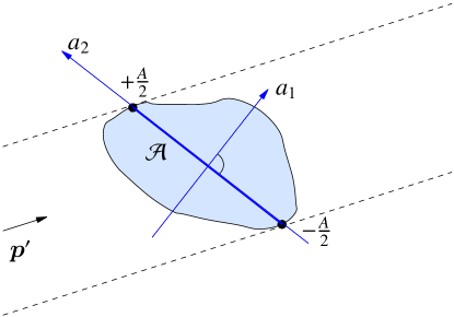
Figure 1: Two-dimensional geometry of atom diffraction from a diffraction object (bar) of finite thickness. The incident momentum of the atom is denoted by $\bm{p}^{\prime}$. The straight shadow line $\mathcal{A}$, which plays the role of the silhouette, divides the bar into an “illuminated” part and a “shadowed” part. Also drawn is the adapted coordinate system $(a_{1},a_{2})$ with the $a_{2}$-axis centered along the shadow line.

III Atom diffraction from a deep grating

III.1 The atom slit function of the deep grating

In diffraction experiments one often employs transmission gratings to enhance the measurable diffraction peak intensities by a factor of $N^{2}$, where $N$ is the number of coherently illuminated bars. One grating bar is simply a special case of the general scattering object considered in the previous section. In the following we arrange $N$ identical bars to create a regularly spaced periodic transmission grating. While the simplest and most familiar situation in which the bars are aligned along their common shadow line ($a_{2}$-axis, cf. Fig. 1) is treated in virtually every textbook on optics (e.g. Ref. Born and Wolf (1959)), we are not aware of a more general treatment where the individual shadow lines are not parallel to the alignment axis. This situation arises naturally, however, for diffraction from a grating with bars of finite thickness at non-zero angle of incidence (cf. Fig. 2). We note that apart from the period an additional length scale of the grating is given by the distance between the bars. Depending on the angle of incidence the (projected) distance can become small or even zero. The diffraction condition (1), which must hold for all length scales, therefore also imposes a limit on the maximal angle of incidence.

Under the diffraction condition the transition amplitude of a grating of $N$ bars with period $d$ along the $x_{2}$-axis can be written as the coherent sum of the spatially translated amplitudes of each bar:

$$t^{\text{at}{(2)}}_{\text{gra}}(\bm{p};\bm{p}^{\prime}) =\sum_{n=0}^{N-1}e^{-i(n-\frac{1}{2}(N-1))\Delta p_{2}d/\hbar}\ t^{\text{at}{(2)}}(\bm{p};\bm{p}^{\prime})$$ (12a)

$$=H_{N}(\Delta p_{2})\ t^{\text{at}{(2)}}(\bm{p};\bm{p}^{\prime}).$$ (12b)

In the second line, the sum has been carried out and replaced by the grating function Born and Wolf (1959)

$$H_{N}(\Delta p_{2})=\frac{\sin(\Delta p_{2}dN/2\hbar)}{\sin(\Delta p_{2}d/2\hbar)}$$ (13)

whose argument is the momentum transfer along the direction of periodicity $x_{2}$. Eq. (12) yields, in principle, a satisfactory description of the diffraction problem in terms of atom scattering from a bar. The literature on optics, however, commonly adapts a complementary point of view by focusing on the apertures (slits) between the bars rather than on the aperture stops (bars) themselves. This is expressed, for example, by the Kirchhoff integral of optics Born and Wolf (1959). In recent work this viewpoint has also proven very useful in the field of atom and molecule diffraction from a transmission grating: small quantum mechanical effects such as the van der Waals interaction Grisenti et al. (1999); Brühl et al. (2002) between the atoms in the beam and the grating as well as the finite size of the helium dimer Grisenti et al. (2000a) manifest themselves as an apparent reduction of the slit width of the grating. In these articles the respective quantities could be determined quite precisely by comparison of the reduced slit width with the true geometrical slit width. Unlike for grating diffraction at normal incidence, however, it is initially not evident how to define a slit in the case of non-normal incidence: the correct choice may depend on the angle of incidence. We provide, therefore, a mathematical prescription which converts Eq. (12) into an expression in the style of the Kirchhoff integral.

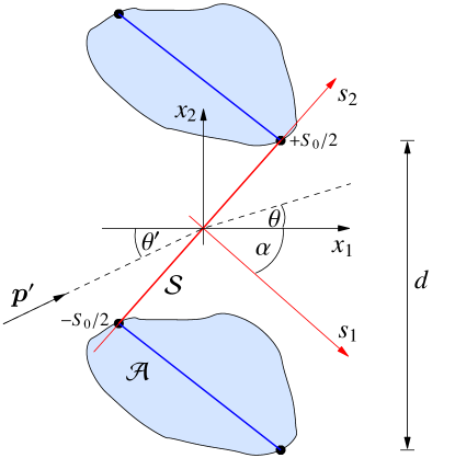
Figure 2: Geometry of atom diffraction from a grating of identical deep bars with period $d$ along the $x_{2}$ direction. The slit line $\mathcal{S}$, which connects the shadow lines $\mathcal{A}$ of adjacent bars, provides a generalization of the notion of a slit at normal incidence. It lends itself to the application of the Huygens principle. Also drawn is the adapted coordinate system $(s_{1},s_{2})$ with the $s_{2}$-axis centered along the slit line and the angle $\alpha$ by which the coordinate systems $(x_{1},x_{2})$ and $(s_{1},s_{2})$ are rotated with respect to each other.

This is achieved by introducing, between every pair of adjacent bars, a new coordinate system $(s_{1},s_{2})$ as depicted in Fig. 2 such that the $s_{2}$-axis meets the boundaries of the two bars at their respective shadow lines. The length of the resulting straight “slit line” $\mathcal{S}$ will be denoted by $S_{0}$. We now substitute the integration variable $a_{2}$ of Eq. (11a) by

$$s_{2}=\frac{\Delta p_{a_{2}}}{\Delta p_{s_{2}}}\left(a_{2}\pm\frac{A}{2}\right)\pm\frac{S_{0}}{2}\quad\mbox{as}\quad a_{2}\lessgtr 0$$

where $\Delta p_{s_{2}}$ denotes the momentum transfer parallel to the $s_{2}$-axis. Similarly, we denote the components of the incident and outgoing momenta with respect to the $s_{1}$-axis by $p^{\prime}_{s_{1}}$ and $p_{s_{1}}$, respectively. (An explicit expression for these momentum components in terms of the geometry of the grating will be given below in Eqs. (27) and (28) for the transmission grating of Fig. 4.) Using the identities

$$\Delta p_{a_{2}}A+\Delta p_{s_{2}}S_{0} = \Delta p_{2}d\ ,$$ (14a)

$$\frac{p_{a_{1}}+p^{\prime}_{a_{1}}}{\Delta p_{a_{2}}}=\frac{p_{s_{1}}+p^{\prime}_{s_{1}}}{\Delta p_{s_{2}}} = \frac{p_{1}+p^{\prime}_{1}}{\Delta p_{2}}\ ,$$ (14b)

which hold because of energy conservation, and the abbreviation $D=d\Delta p_{2}/\Delta p_{s_{2}}$, the transition amplitude of the single bar Eq. (11a) becomes

$$t^{\text{at}{(2)}}(\bm{p};\bm{p}^{\prime})=-\frac{i}{2}\frac{p_{s_{1}}+p^{\prime}_{s_{1}}}{(2\pi)^{2}m\hbar}\left\{\ e^{i\Delta p_{2}d/2\hbar}\int_{{S_{0}}/2}^{{D}/2}ds_{2}\ e^{-i\Delta p_{s_{2}}s_{2}/\hbar}\right.$$

$$+\left.e^{-i\Delta p_{2}d/2\hbar}\int_{-{D}/2}^{-{S_{0}}/2}ds_{2}\ e^{-i\Delta p_{s_{2}}s_{2}/\hbar}\ \right\}.\hskip 14.22636pt$$ (15)

Keeping in mind that the integration variable $s_{2}$ was substituted for $a_{2}$ for a single bar the following geometrical interpretation is possible: in the integral from $S_{0}/2$ to $D/2$ in Eq. (15) the variable $s_{2}$ represents the position along the upper half of the slit line $\mathcal{S}$ on one side of the bar; similarly, in the integral running from $-D/2$ to $-S_{0}/2$, $s_{2}$ is the position along the lower half of the next slit line at the other side the bar. Inserting Eq. (15) into Eq. (12a) the half slit lines of the $N$ adjacent bars can be joined to yield $N-1$ slits between them. Collecting all terms and introducing a “slit function”,

$$a^{\text{at}}(\bm{p}^{\prime};\Delta p_{s_{2}})=\int_{-{D}/2}^{{D}/2}ds_{2}\ \exp\left(-i\Delta p_{s_{2}}s_{2}/\hbar\right)\ \tau^{\text{at}}(\bm{p}^{\prime};s_{2}),$$ (16)

where the transmission function $\tau^{\text{at}}(\bm{p}^{\prime};s_{2})$ inserted here is unity inside the slit $\mathcal{S}$ and zero otherwise, the transition amplitude of the grating can be written, for $N\gg 1$, as

$$t^{\text{at}{(2)}}_{\text{gra}}(\bm{p};\bm{p}^{\prime})\simeq-\frac{i}{2}\frac{p_{s_{1}}+p^{\prime}_{s_{1}}}{(2\pi)^{2}m\hbar}$$

$$\times \left\{\ \frac{\sin\left(\Delta p_{2}Nd/2\hbar\right)}{\Delta p_{s_{2}}/2\hbar}-H_{N-1}(\Delta p_{2})\ a^{\text{at}}(\bm{p}^{\prime};\Delta p_{s_{2}})\right\}.$$

The first term in curly brackets is sharply peaked about the forward direction, and in the limit $N\rightarrow\infty$, using Eq. (14b), it simply reduces to $2\pi\hbar\frac{p_{1}}{p_{s_{1}}}\delta(\Delta p_{2})$. The second term, which is a product of the grating function (13) and the slit function (16), generates the familiar diffraction pattern of a grating footnote-HN . The $n$-th order principle diffraction maximum appears at the momentum transfer

$$\Delta p_{2}=\frac{n2\pi\hbar}{d}.$$

Introducing the angle of incidence $\theta^{\prime}$ such that $p^{\prime}_{1}=|\bm{p}^{\prime}|\cos\theta^{\prime}$ and $p^{\prime}_{2}=|\bm{p}^{\prime}|\sin\theta^{\prime}$ (cf. Fig. 2), and equivalently the diffraction angle $\theta$ such that $p_{1}=|\bm{p}|\cos\theta$ and $p_{2}=|\bm{p}|\sin\theta$, the $n$-th order is located at the angle $\theta=\theta_{n}$ satisfying

$$\sin\theta_{n}=\sin\theta^{\prime}+\frac{n2\pi\hbar}{|\bm{p}^{\prime}|d}\ .$$ (18)

Generally, the diffraction intensities are proportional to the scattering matrix element $|\langle\bm{\mathrm{p}}|S|\bm{\mathrm{p}}^{\prime}\rangle|^{2}$ where the components of the outgoing momentum $\bm{p}$ must be evaluated at the angle $\theta_{n}$. Inserting Eq. (III.1) into Eq. (4) one finds, after some algebra,

$$I_{n}=I_{0}\left(\frac{p_{s_{1}}+p^{\prime}_{s_{1}}}{2p^{\prime}_{s_{1}}}\right)^{2}\frac{|a^{\text{at}}\left(\bm{p}^{\prime};\Delta p_{s_{2}}\right)|^{2}}{|a^{\text{at}}\left(\bm{p}^{\prime};0\right)|^{2}},$$ (19)

where the intensity $I_{0}$ of the zeroth diffraction order serves as a normalization constant depending on the experimental counting rate and where, from Eq. (16), $|a^{\text{at}}\left(\bm{p}^{\prime};0\right)|^{2}=S_{0}^{2}$ (in the absence of the van der Waals interaction considered below).

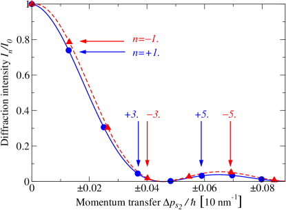
Figure 3: Asymmetric probing of the envelope function by the grating function at non-normal incidence. Both curves show the product $({p_{s_{1}}+p^{\prime}_{s_{1}}})^{2}/({2p^{\prime}_{s_{1}}S_{0}})^{2}|a^{\text{at}}\left(\bm{p}^{\prime};\Delta p_{s_{2}}\right)|^{2}$ as it appears in Eq. (19) versus the momentum transfer $\Delta p_{s_{2}}$. The solid curve refers to the positive values of $\Delta p_{s_{2}}$ on the horizontal axis. The dashed curve refers to the negative values of $\Delta p_{s_{2}}$ which have been mirrored onto the positive axis for comparison. The circles and triangles on top of the solid and the dashed curves, respectively, mark those values of $\Delta p_{s_{2}}$ where the grating function $H_{N}(\Delta p_{2})$ probes the slit function, i.e. where $\Delta p_{2}=n2\pi\hbar/d$ is satisfied for $n=0,\pm 1,\pm 2,\dots$. Their intensities correspond to the measurable diffraction peaks. For the calculation of this figure the grating cross section of Fig. 4 was used with the beam parameters $\theta^{\prime}=21^{\circ}$ and $|\bm{p}^{\prime}|/\hbar=10$ nm^-1.

We now discuss the intensity formula Eq. (19) to explain the origin of the asymmetry of the diffraction pattern. The slit function $a^{\text{at}}\left(\bm{p}^{\prime};\Delta p_{s_{2}}\right)$ is an even function of the momentum transfer component $\Delta p_{s_{2}}$. The geometrical factor $({p_{s_{1}}+p^{\prime}_{s_{1}}})^{2}/({2p^{\prime}_{s_{1}}S_{0}})^{2}$ (the component $p_{s_{1}}$ depends on $\Delta p_{s_{2}}$ through conservation of energy and momentum) can be shown to introduce, for positive incident angle $\theta^{\prime}$, a slight attenuation of the slit function at positive $\Delta p_{s_{2}}$ and likewise an intensification at negative $\Delta p_{s_{2}}$. The product of the slit function and the geometrical factor serves in Eq. (19) as an envelope function which is probed by the grating function at the momentum transfer $\Delta p_{2}$ rather than at $\Delta p_{s_{2}}$. Since $\Delta p_{s_{2}}$ and $\Delta p_{2}$ are not proportional to each other this probing is not symmetric for positive and negative diffraction angles. This is depicted in Fig. 3, and it leads to the characteristic asymmetry of the diffraction pattern of a deep grating at non-normal incidence. Expanding $\Delta p_{s_{2}}$, using Eq. (14b), into a power series in $(\Delta p_{2}/\cos\theta^{\prime})$ through second order,

$$\frac{\Delta p_{s_{2}}}{\cos(\alpha+\theta^{\prime})}\simeq\frac{\Delta p_{2}}{\cos\theta^{\prime}}+\frac{\tan\theta^{\prime}-\tan(\alpha+\theta^{\prime})}{2|\bm{p}^{\prime}|}\left(\frac{\Delta p_{2}}{\cos\theta^{\prime}}\right)^{2},$$ (20)

the leading non-linear term is seen to vanish like $\Delta p_{2}/|\bm{p}^{\prime}|$ relative to the linear term. Accordingly, the asymmetry is less pronounced for smaller diffraction orders, for faster beams and, in the case of molecules, for heavier molecules. While at $|\bm{p}^{\prime}|/\hbar=10\,\text{nm}^{-1}$ (corresponding to a ⁴He beam at $v\approx 160\,$m/s), as seen in Fig. 3, the quadratic term in Eq. (20) is responsible for a $\pm 8\%$ deviation of the positive and negative fifth diffraction orders, respectively, its contribution reduces to $\pm 0.7\%$ at $v=1800\,$m/s. This smallness explains why the asymmetry has previously been missed (cf. Fig. 5 in Ref. Grisenti et al. (2000b)). Clearly, in the thin grating limit $\alpha\rightarrow 0$ the mirror symmetry is recovered in Eq. (20).

In the derivation so far no comment has been made about the inclusion of the attractive van der Waals interaction between the atom and the grating. It can be accounted for through the transmission function $\tau^{\text{at}}(\bm{p}^{\prime};s_{2})$ in the slit function (16) as outlined in Appendix A and in Refs. Hegerfeldt and Köhler (2000a); Grisenti et al. (1999). Unlike the case of normal incidence, at non-normal incidence the influence of the van der Waals interaction may be different on each side of the slit, introducing, in principle, an additional source of asymmetry to the diffraction pattern. Numerical comparisons using the explicit expression of Appendix A for the transmission function demonstrate, however, that this effect is minor.

III.2 The atom diffraction pattern of the deep grating

The quantitative evaluation of experimental diffraction data requires to determine a set of parameters describing the geometry of the particular grating (cf. Fig. 4) as well as the van der Waals interaction coefficient $C_{3}$ (cf. appendix A).

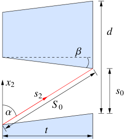
Figure 4: Geometrical cross section of a custom diffraction grating as it has been used in matter diffraction experiments Grisenti et al. (1999); Grisenti et al. (2000a). The parameters and their typical values are: period $d=100$ nm, slit width $s_{0}=60$ nm, thickness $t=120$ nm, and wedge angle $\beta=6^{\circ}$. The angle by which the coordinate systems $(x_{1},x_{2})$ and $(s_{1},s_{2})$ are rotated with respect to each other satisfies $\cot\alpha=\tan\beta+s_{0}/t$ and $S_{0}\sin\alpha=t$. At the above parameters $\alpha\approx 58^{\circ}$. The characteristic shape of the bars is reminiscent of the lithographic production process Savas et al. (1995).

Previous work has shown that an immediate numerical fit of Eq. (19) to experimental data does not reliably determine these parameters. Analogous to the procedure developed in Ref. Grisenti et al. (1999) for diffraction at normal incidence we therefore introduce a two-term cumulant approximation of the slit function. To this end we rewrite Eq. (16) as

$$a^{\text{at}}({\bm{p}}^{\prime};\Delta p_{s_{2}})=\frac{\hbar}{i\Delta p_{s_{2}}}$$

$$\times\ \left\{e^{i\Delta p_{s_{2}}S_{0}/2\hbar}\ \Phi^{-}\left(\frac{\Delta p_{s_{2}}}{\hbar}\right)-e^{-i\Delta p_{s_{2}}S_{0}/2\hbar}\ \Phi^{+}\left(\frac{\Delta p_{s_{2}}}{\hbar}\right)\right\}$$ (21)

where the functions $\Phi^{+}(\kappa)$ and $\Phi^{-}(\kappa)$ are defined by

$$\Phi^{\pm}(\kappa)=\frac{\mp 1}{\tau^{\text{at}}\left({\bm{p}}^{\prime};0\right)}\int_{0}^{{S_{0}}/2}d\xi\ e^{\pm i\kappa\xi}\ {\tau^{\text{at}}}^{\prime}\left({\bm{p}}^{\prime};\pm\left(\frac{S_{0}}{2}-\xi\right)\right).$$ (22)

Here, ${\tau^{\text{at}}}^{\prime}(\bm{p}^{\prime};s_{2})$ denotes the derivative of the transmission function with respect to its position argument. As $\Phi^{\pm}(0)=1$ the logarithm of $\Phi^{\pm}(\kappa)$ can be expanded into a power series of the form

$$\ln\Phi^{\pm}(\kappa)=\sum_{j=1}^{\infty}\frac{(\pm i\kappa)^{j}}{j!}R^{\pm}_{j}.$$ (23)

The complex numbers $R^{\pm}_{1}$ and $R^{\pm}_{2}$, which are known as the first two cumulants, are uniquely determined by Eqs. (22) and (23). One finds

$$R^{\pm}_{1} = \frac{S_{0}}{2}-\int_{0}^{{S_{0}}/2}d\xi\ \tau^{\text{at}}\left({\bm{p}}^{\prime};\pm\left(\frac{S_{0}}{2}-\xi\right)\right)$$ (24)

and

$$R^{\pm}_{2}=\left(\frac{S_{0}}{2}\right)^{2}-\left(R^{\pm}_{1}\right)^{2}-2\int_{0}^{S_{0}/2}d\xi\ \xi\ \tau^{\text{at}}\left({\bm{p}}^{\prime};\pm\left(\frac{S_{0}}{2}-\xi\right)\right).$$ (25)

Using the explicit form of the transmission function derived in the appendix the length scale of the cumulants can be shown to be set by the parameter $\sqrt{C_{3}/(\hbar v)}$. For helium and a SiN_x grating $C_{3}\approx 0.1\,$meV nm³ Grisenti et al. (1999). Therefore, for the purposes of this work it is sufficient to truncate the expansion Eq. (23) after the second order. Inserting the first two terms into the slit function Eq. (21) and introducing the four quantities

$$S_{\text{eff}}=S_{0}-\text{\,Re\,}(R^{+}_{1}+R^{-}_{1}), \Delta=\text{\,Im\,}(R^{+}_{1}+R^{-}_{1}),$$

$$\Gamma=\text{\,Im\,}(R^{+}_{1}-R^{-}_{1}), \Sigma=\sqrt{\frac{1}{2}\text{\,Re\,}(R^{+}_{2}+R^{-}_{2})},$$

the $n$-th order diffraction intensity relative to the zeroth order is given, within this approximation, by

$$\frac{I_{n}}{I_{0}}= \left[\frac{p_{s_{1}}+p^{\prime}_{s_{1}}}{2p^{\prime}_{s_{1}}\sqrt{S_{\text{eff}}^{2}+\Delta^{2}}}\right]^{2}\exp\left[-(\Delta p_{s_{2}}\Sigma)^{2}/\hbar^{2}\right]\ \exp[-\Gamma\Delta p_{s_{2}}/\hbar]$$

$$\ \times\ \frac{\sin^{2}[\Delta p_{s_{2}}S_{\text{eff}}/2\hbar]+\sinh^{2}[\Delta p_{s_{2}}\Delta/2\hbar]}{\left[\Delta p_{s_{2}}/2\hbar\right]^{2}}.$$ (26)

Here, the momentum components are to be taken explicitly at the angles

$$p_{s_{1}}=|\bm{p}^{\prime}|\cos(\alpha+\theta_{n})$$ (27a)

$$p^{\prime}_{s_{1}}=|\bm{p}^{\prime}|\cos(\alpha+\theta^{\prime})$$ (27b)

and the momentum transfer is given by

$$\Delta p_{s_{2}}=|\bm{p}^{\prime}|\left[\sin(\alpha+\theta_{n})-\sin(\alpha+\theta^{\prime})\right]$$ (28)

where $\alpha$ denotes the angle shown in Fig. 4 by which the coordinate system $(s_{1},s_{2})$ is rotated with respect to $(x_{1},x_{2})$. The diffraction intensity formula (26) is, though more complicated, reminiscent of the result for normal incidence derived in Ref. Grisenti et al. (1999): The long fraction involving the sine of $S_{\text{eff}}$ resembles the Kirchhoff slit function for a slit of “effective width” $S_{\text{eff}}$ whose intensity zeros, though, are removed by the hyperbolic sine function involving $\Delta$. The Gaussian exponential reflects the suppression of higher diffraction orders. The asymmetry $I_{n}\neq I_{-n}$ of the diffraction pattern is now embodied by the asymmetry in $\Delta p_{s_{2}}$ as a function of $n$ in Eq. (28). The second exponential in Eq. (26) accounts for the minor additional asymmetry in the diffraction pattern due to the different influence of the van der Waals interaction on both sides of the bar. A comparison of the diffraction intensities calculated from Eq. (19) and the approximation (26) is displayed in Fig. 5.

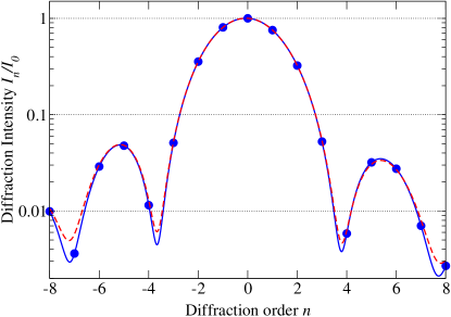
Figure 5: Diffraction intensities of a Helium atom beam at $v=500$ m/s from a $d=100$ nm transmission grating as displayed in Fig. 4 at $\theta^{\prime}=21^{\circ}$ angle of incidence. The solid curve was calculated using Eq. (19), the dashed curve shows the two-term cumulant approximation (26). To guide the eye these functions are shown continuously. The circles on top of the solid curve at integer $n$ mark the experimentally accessible diffraction orders $I_{n}/I_{0}$.

By a numerical fit of Eq. (26) to experimental diffraction data the effective slit width $S_{\text{eff}}$, amongst the other parameters, can be determined accurately and allows for further comparison between theory and experiment along the lines of Ref. Grisenti et al. (1999). For completeness, we note that

$$S_{\text{eff}}=S_{0}-\text{\,Re\,}\int_{-{S_{0}}/2}^{{S_{0}}/2}ds_{2}\left[1-\tau^{\text{at}}({\bm{p}}^{\prime};s_{2})\right].$$ (29)

This means that the geometrical slit width $S_{0}$ appears to be reduced by the average deviation from unity of the transmission function $\tau^{\text{at}}({\bm{p}}^{\prime};s_{2})$.

IV Trimer diffraction theory

A trimer, in the scope of this article, is a three-atomic molecule which is weakly bound by pair interactions footnote-othertrimers . Again, the atoms themselves are treated as point particles. An additional three-body interaction between the atoms is assumed to be negligible. Central to later applications will be the helium trimer ⁴He₃ in which case at least these assumptions are expected to be valid Røeggen and Almlöf (1995).

IV.1 Three-body bound states

The masses of the three atoms at positions $\bm{\mathrm{r}}_{i}$, for $i=1,2,3$, will be denoted by $m_{i}$ and are assumed to be of the same order of magnitude. The interaction between atom $j$ and $k$ is modeled by a potential $v_{jk}(|\bm{\mathrm{r}}^{(jk)}|)$ where $\bm{\mathrm{r}}^{(jk)}=\bm{\mathrm{r}}_{j}-\bm{\mathrm{r}}_{k}$ is the relative coordinate.

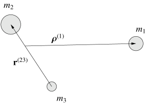
Figure 6: One of three possible sets of Jacobi coordinates. The vector $\bm{\mathrm{\rho}}^{(1)}$ points from the center of mass of the subsystem $(23)$ to atom 1. The vector $\bm{\mathrm{r}}^{(23)}$ is the relative coordinate of the subsystem. The coordinate $\bm{\mathrm{R}}$ (not shown) corresponds to the center of mass position and is, therefore, identical for all three sets.

We introduce the Jacobi coordinates $\bm{\mathrm{R}},\bm{\mathrm{\rho}}^{(i)},\bm{\mathrm{r}}^{(jk)}$ sketched in Fig. 6, which can be expressed in block matrix form as

$$\left(\begin{array}[]{l}\bm{\mathrm{R}}\\ \bm{\mathrm{\rho}}^{(i)}\\ \bm{\mathrm{r}}^{(jk)}\end{array}\right)=\left(\begin{array}[]{rrr}\frac{m_{i}}{M}\mathbf{1}&\frac{m_{j}}{M}\mathbf{1}&\frac{m_{k}}{M}\mathbf{1}\\ \mathbf{1}&-\frac{m_{j}}{m_{j}+m_{k}}\mathbf{1}&-\frac{m_{k}}{m_{j}+m_{k}}\mathbf{1}\\ \mathbf{0}&\mathbf{1}&-\mathbf{1}\end{array}\right)\left(\begin{array}[]{l}\bm{\mathrm{r}}_{i}\\ \bm{\mathrm{r}}_{j}\\ \bm{\mathrm{r}}_{k}\end{array}\right),$$ (30)

where $\mathbf{1}$ and $\mathbf{0}$ denote the $3\times 3$ unit and zero matrix, respectively, and $M=m_{1}+m_{2}+m_{3}$ is the total mass. It is sufficient to restrict the combinations of indices to the ascending permutations

$$(ijk)=(123),(231),(312).$$ (31)

The transformation between different sets of Jacobi coordinates can be derived from Eq. (30). It takes the form

$$\left(\begin{array}[]{l}\bm{\mathrm{R}}\\ \bm{\mathrm{\rho}}^{(j)}\\ \bm{\mathrm{r}}^{(ki)}\end{array}\right)=\mathcal{J}^{(ji)}\left(\begin{array}[]{l}\bm{\mathrm{R}}\\ \bm{\mathrm{\rho}}^{(i)}\\ \bm{\mathrm{r}}^{(jk)}\end{array}\right),$$ (32)

where the block matrix $\mathcal{J}^{(ji)}$ is given by

$$\mathcal{J}^{(ji)}=\left(\begin{array}[]{rrr}\mathbf{1}&\mathbf{0}&\mathbf{0}\\ \mathbf{0}&-\frac{m_{i}}{m_{i}+m_{k}}\mathbf{1}&\frac{m_{k}M}{(m_{j}+m_{k})(m_{k}+m_{i})}\mathbf{1}\\ \mathbf{0}&-\mathbf{1}&-\frac{m_{j}}{m_{j}+m_{k}}\mathbf{1}\end{array}\right).$$ (33)

The three matrices $\mathcal{J}^{(ji)}$ satisfy the relations $\det\mathcal{J}^{(ji)}=1$ and $\mathcal{J}^{(ji)}\mathcal{J}^{(ik)}\mathcal{J}^{(kj)}=\mathbf{1}$. Expressed in Jacobi coordinates the Hamilton operator for a free trimer is given by $H_{0}+V$ where

$$H_{0}= \ \frac{1}{2M}\bm{\mathrm{\hat{P}}}^{2}+\frac{M}{2m_{i}(m_{j}+m_{k})}{\bm{\mathrm{\hat{q}}}^{(i)\,2}}+\frac{m_{j}+m_{k}}{2m_{j}m_{k}}{\bm{\mathrm{\hat{p}}}^{(jk)\,2}}$$

$$V=\ v_{ij}\left(\left|\hat{\bm{\mathrm{\rho}}}^{(i)}-\frac{m_{k}}{m_{j}+m_{k}}\bm{\mathrm{\hat{r}}}^{(jk)}\right|\right)+v_{jk}\left(\left|\bm{\mathrm{\hat{r}}}^{(jk)}\right|\right)$$

$$+\ v_{ki}\left(\left|\hat{\bm{\mathrm{\rho}}}^{(i)}+\frac{m_{j}}{m_{j}+m_{k}}\bm{\mathrm{\hat{r}}}^{(jk)}\right|\right).$$ (34)

Here, $\bm{\mathrm{P}},\bm{\mathrm{q}}^{(i)}$, and $\bm{\mathrm{p}}^{(jk)}$ are the conjugate momenta associated with $\bm{\mathrm{R}},\bm{\mathrm{\rho}}^{(i)}$, and $\bm{\mathrm{r}}^{(jk)}$, respectively. Denoting the eigenstates of the center of mass momentum $\hat{\bm{\mathrm{P}}}$ by $|\bm{\mathrm{P}}\rangle$ the full trimer states can be written in product form $|\bm{\mathrm{P}},\phi_{\gamma}\rangle\equiv|\bm{\mathrm{P}}\rangle|\phi_{\gamma}\rangle$ satisfying

$$[H_{0}+V]|\bm{\mathrm{P}},\phi_{\gamma}\rangle=E|\bm{\mathrm{P}},\phi_{\gamma}\rangle$$ (35)

with energy eigenvalues

$$E=\frac{|\bm{\mathrm{P}}|^{2}}{2M}+E_{\gamma}$$ (36)

where $E_{\gamma}$ is the negative binding energy of the trimer bound state $|\phi\rangle_{\gamma}$.

The representation of a trimer state by its wave function depends on the particular set of Jacobi coordinates. Denoting the common eigenstates of the relative momentum operators $\bm{\mathrm{\hat{q}}}^{(i)}$ and $\bm{\mathrm{\hat{p}}}^{(jk)}$ by $|\bm{\mathrm{q}},\bm{\mathrm{p}}\rangle_{i,jk}$, where $\bm{\mathrm{q}}$ and $\bm{\mathrm{p}}$ are the corresponding eigenvalues, we introduce momentum space wave functions by

$$\phi_{\gamma}^{(i,jk)}(\bm{\mathrm{q}},\bm{\mathrm{p}})=\ _{i,jk}\langle\bm{\mathrm{q}},\bm{\mathrm{p}}|\phi_{\gamma}\rangle.$$ (37)

Because of the transformation Eq. (32) wave functions with respect to different sets of Jacobi coordinates can be chosen to satisfy the transformation relation

$$\phi_{\gamma}^{(i,jk)}(\bm{\mathrm{q}}^{(i)},\bm{\mathrm{p}}^{(jk)})=\phi_{\gamma}^{(j,ki)}(\bm{\mathrm{q}}^{(j)},\bm{\mathrm{p}}^{(ki)}).$$ (38)

The corresponding configuration space wave functions $\phi_{\gamma}^{(i,jk)}(\bm{\mathrm{\rho}},\bm{\mathrm{r}})$ are defined analogously. In order not to overload the notation we will omit in the following, where possible, the indices of the relative coordinates: if not denoted otherwise we implicitly use $(ijk)=(123)$ whence $\bm{\mathrm{\rho}}\equiv\bm{\mathrm{\rho}}^{(1)}$, $\bm{\mathrm{r}}\equiv\bm{\mathrm{r}}^{(23)}$ and $\bm{\mathrm{q}}\equiv\bm{\mathrm{q}}^{(1)}$, $\bm{\mathrm{p}}\equiv\bm{\mathrm{p}}^{(23)}$.

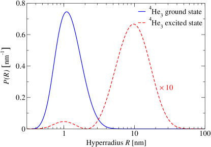
Figure 7: Hyperradial probability densities $P(R)$ according to Eq. (39) of the two theoretically predicted bound states of the helium trimer ⁴He₃. The states were calculated numerically using the momentum space Faddeev equations Faddeev (1961); Sitenko (1971) in the unitary pole approximation Lovelace (1964) based on the TTY potential Tang et al. (1995) for the helium-helium interaction. Clearly, the excited state, with its expectation value of the hyperradius of $\sqrt{\mu_{0}/m}\left\langle R\right\rangle_{\text{e}}=10.1\,$nm, is spatially more extended by almost one order of magnitude than the ground state with $\sqrt{\mu_{0}/m}\left\langle R\right\rangle_{\text{g}}=1.1\,$nm. The scaling of the horizontal axis is logarithmic.

Since the discovery of the Efimov effect Efimov (1970) in 1970 the helium trimer ⁴He₃ has received much attention Lim et al. (1977); Huber and Lim (1977); Nakaichi-Maeda and Lim (1983); Fedorov and Jensen (1993); Nielsen et al. (1998); Motovilov et al. (1997); Kolganova et al. (1998); Roudnev and Yakovlev (2000); Motovilov et al. (2001); Esry et al. (1996); Bruch (1999); Barletta and Kievsky (2001); Lewerenz (1997); Røeggen and Almlöf (1995); Braaten and Hammer (2003); Braaten et al. (2003); Yamashita et al. (2003); Hegerfeldt and Köhler (2000b). This trimer is predicted to possess, apart from its quite tightly bound ground state ($E_{\text{g}}=-126$ mK), a weakly bound Efimov-type excited state ($E_{\text{e}}=-2.3$ mK) Barletta and Kievsky (2001). As both states have zero total angular momentum the corresponding wave functions only depend on three coordinates which may be taken as $\rho=|\bm{\mathrm{\rho}}|,r=|\bm{\mathrm{r}}|$, and the angle between $\bm{\mathrm{\rho}}$ and $\bm{\mathrm{r}}$. A common way to visualize trimer wave functions is to draw the hyperspherical probability density $P(R)$: The hyperradius $R$, which is independent of the choice of the set of Jacobi coordinates, is defined as $\mu_{0}R(\rho,r)^{2}=\frac{2}{3}m\rho^{2}+\frac{1}{2}mr^{2}$ and the corresponding probability density can be calculated according to

$$P(R)=\int d^{3}\rho d^{3}r|\phi_{\gamma}(\bm{\mathrm{\rho}},\bm{\mathrm{r}})|^{2}\delta(R(\rho,r)-R).$$ (39)

The purpose of the “mass” parameter $\mu_{0}$ is to ensure that the unit of $R$ is length. The numerical value of $\mu_{0}$ is, in principle, arbitrary as it simply scales $R$. Fig. 7 displays the hyperradial probability densities for the two helium trimer states, using $\mu_{0}/m=\frac{1}{2}$, which were calculated numerically from the momentum space Faddeev equations Faddeev (1961); Sitenko (1971) in the unitary pole approximation Lovelace (1964) based on the TTY potential Tang et al. (1995).

IV.2 Scattering theory approach to trimer diffraction

We now proceed to the diffraction of a trimer from an external potential

$$W(\bm{\mathrm{r}}_{1},\bm{\mathrm{r}}_{2},\bm{\mathrm{r}}_{3})=W_{1}(\bm{\mathrm{r}}_{1})+W_{2}(\bm{\mathrm{r}}_{2})+W_{3}(\bm{\mathrm{r}}_{3})$$ (40)

where the $W_{i}(\bm{\mathrm{r}}_{i})$ are the interactions of the individual atoms with the diffraction object. The full Hamilton operator is given by

$$H=H_{0}+V+W.$$ (41)

By virtue of this structure, which is formally identical to that of dimer diffraction Hegerfeldt and Köhler (1998), we may carry over the fundamental algebraic relations from previous work. Introducing, as in Ref. Hegerfeldt and Köhler (1998), the resolvents

$$G_{0}(z) = \left[z-H_{0}\right]^{-1}$$ (42a)

$$G_{V}(z) = \left[z-H_{0}-V\right]^{-1}$$ (42b)

$$G_{W}(z) = \left[z-H_{0}-W\right]^{-1}$$ (42c)

and the two-body $T$ matrices in three-body space,

$$T_{V}(z) = V+VG_{V}(z)V$$ (43)

$$T_{W}(z) = W+WG_{W}(z)W$$ (44)

for the potentials $V$ and $W$, an AGS type Alt et al. (1967) transition operator $U_{VV}$ can be derived which satisfies the equation

$$U_{VV}=T_{W}+T_{W}G_{0}T_{V}G_{0}U_{VV}.$$ (45)

In particular, the transition amplitude is given by the matrix element of this transition operator Hegerfeldt and Köhler (1998),

$$t(\bm{\mathrm{P}},\phi_{\gamma};\bm{\mathrm{P}}^{\prime},\phi_{\gamma^{\prime}})=\langle\bm{\mathrm{P}},\phi_{\gamma}|U_{VV}(E^{\prime}+i0)|\bm{\mathrm{P}}^{\prime},\phi_{\gamma^{\prime}}\rangle,$$ (46)

and it determines the $S$ matrix associated with $H$ as

$$\langle\bm{\mathrm{P}},\phi_{\gamma}|S_{VV}|\bm{\mathrm{P}}^{\prime},\phi_{\gamma^{\prime}}\rangle=\ \delta^{(3)}(\bm{\mathrm{P}}-\bm{\mathrm{P}}^{\prime})\delta_{\gamma\gamma^{\prime}}$$

$$-2\pi i\delta(E-E^{\prime})t(\bm{\mathrm{P}},\phi_{\gamma};\bm{\mathrm{P}}^{\prime},\phi_{\gamma^{\prime}}).$$ (47)

We shall in the following impose the condition

$$|E_{\gamma}|,|\langle\phi_{\gamma}|V|\phi_{\gamma}\rangle|\ll\frac{|\bm{\mathrm{P}}|^{2}}{2M},\frac{|\bm{\mathrm{P}}^{\prime}|^{2}}{2M}$$ (48)

which ensures that the internal energies of the trimer (both binding energy and potential energy) are much smaller than the external energy associated with the center of mass motion. For a helium trimer beam at an incident beam velocity of $v=500$ m/s, for example, the center of mass kinetic energy ${|\bm{\mathrm{P}}^{\prime}|^{2}}/({2M})\approx 16\,$meV (corresponding to $180$ K) exceeds the trimer ground state energy by more than three orders of magnitude. Using the Schrödinger equation for bound trimer wave functions $\phi_{\gamma}(\bm{\mathrm{q}},\bm{\mathrm{p}})$ the condition (48) can be shown to entail the relations

$$|\bm{\mathrm{q}}|\ll|\bm{\mathrm{P}}|,|\bm{\mathrm{P}}^{\prime}|\quad\mbox{and}\quad|\bm{\mathrm{p}}|\ll|\bm{\mathrm{P}}|,|\bm{\mathrm{P}}^{\prime}|.$$ (49)

These state that the wave functions of the trimer are concentrated in momentum space at relative momenta far smaller than the center of mass momentum.

Under the conditions (48) and (49) an approximation of the equation for $U_{VV}$ (45) to lowest order is possible and sufficient (Glöckle, 1983, chap. 3.4) whence the transition amplitude becomes

$$t(\bm{\mathrm{P}},\phi_{\gamma};\bm{\mathrm{P}}^{\prime},\phi_{\gamma^{\prime}})\simeq\langle\bm{\mathrm{P}},\phi_{\gamma}|T_{W}(E^{\prime}+i0)|\bm{\mathrm{P}}^{\prime},\phi_{\gamma^{\prime}}\rangle.$$ (50)

We note that within this approximation the trimer binding potential $V$ is only implicitly contained through the bound states $|\phi\rangle_{\gamma}$ and $|\phi\rangle_{\gamma^{\prime}}$. The evaluation of the right hand side of Eq. (50) is nontrivial. A series of approximations, all accurate within the condition (48), may however be applied to simplify the transition amplitude. As the first step, the matrix element of $T_{W}(E^{\prime}+i0)$ can be shown to vary slowly under a variation of $E^{\prime}$ on the scale of the binding energies $E_{\gamma^{\prime}}$. This allows to replace the energy argument of $T_{W}$ in Eq. (50) by the sum $E^{\prime}_{1}+E^{\prime}_{2}+E^{\prime}_{3}$ where $E^{\prime}_{i}=|\bm{\mathrm{p}}^{\prime}_{i}|^{2}/2m_{i}$ are the energies of the free atoms. Introducing two complete sets of states Eq. (50) becomes

$$t(\bm{\mathrm{P}},\phi_{\gamma};\bm{\mathrm{P}}^{\prime},\phi_{\gamma^{\prime}})\simeq\int d^{3}q\,d^{3}p\,d^{3}q^{\prime}d^{3}p^{\prime}\,\phi_{\gamma}^{*}(\bm{\mathrm{q}},\bm{\mathrm{p}})\phi_{\gamma^{\prime}}(\bm{\mathrm{q}}^{\prime},\bm{\mathrm{p}}^{\prime})\$$ (51)

$$\times \langle\bm{\mathrm{p}}_{1},\bm{\mathrm{p}}_{2},\bm{\mathrm{p}}_{3}|T_{W}(E^{\prime}_{1}+E^{\prime}_{2}+E^{\prime}_{3}+i0)|\bm{\mathrm{p}}^{\prime}_{1},\bm{\mathrm{p}}^{\prime}_{2},\bm{\mathrm{p}}^{\prime}_{3}\rangle.$$

Using Eqs. (42) and (44) the algebraic relation $T_{W}(z)G_{0}(z)=WG_{W}(z)$ can be shown to hold. Inserting this relation the matrix element of $T_{W}(E^{\prime}_{1}+E^{\prime}_{2}+E^{\prime}_{3}+i0)$ is replaced by

$$\langle\bm{\mathrm{p}}_{1},\bm{\mathrm{p}}_{2},\bm{\mathrm{p}}_{3}|W|\bm{\mathrm{p}}^{\prime}_{1},\bm{\mathrm{p}}^{\prime}_{2},\bm{\mathrm{p}}^{\prime}_{3},+\rangle$$ (52)

where $|\bm{\mathrm{p}}^{\prime}_{1},\bm{\mathrm{p}}^{\prime}_{2},\bm{\mathrm{p}}^{\prime}_{3},+\rangle\equiv|\bm{\mathrm{p}}^{\prime}_{1},+\rangle|\bm{\mathrm{p}}^{\prime}_{2},+\rangle|\bm{\mathrm{p}}^{\prime}_{3},+\rangle$ is the scattering state of three independent atoms associated with the potential $W(\bm{\mathrm{r}}_{1},\bm{\mathrm{r}}_{2},\bm{\mathrm{r}}_{3})$. Splitting $W$ according to Eq. (40) into the individual potentials $W_{i}(\bm{\mathrm{r}}_{i})$ and using the Lippmann-Schwinger Eq. (2) the matrix element (52) can be expressed by the known atom transition amplitudes (3):

$$\langle\bm{\mathrm{p}}_{1},\bm{\mathrm{p}}_{2},\bm{\mathrm{p}}_{3}|W|\bm{\mathrm{p}}^{\prime}_{1},\bm{\mathrm{p}}^{\prime}_{2},\bm{\mathrm{p}}^{\prime}_{3},+\rangle=t^{\text{at}}_{1}(\bm{\mathrm{p}}_{1};\bm{\mathrm{p}}^{\prime}_{1})\ \delta^{(3)}(\bm{\mathrm{p}}_{2}-\bm{\mathrm{p}}^{\prime}_{2})$$

$$\times\ \delta^{(3)}(\bm{\mathrm{p}}_{3}-\bm{\mathrm{p}}^{\prime}_{3})+t^{\text{at}}_{1}(\bm{\mathrm{p}}_{1};\bm{\mathrm{p}}^{\prime}_{1})\ \delta^{(3)}(\bm{\mathrm{p}}_{2}-\bm{\mathrm{p}}^{\prime}_{2})\ t^{\text{at}}_{3}(\bm{\mathrm{p}}_{3};\bm{\mathrm{p}}^{\prime}_{3})$$

$$\times\ \left[\frac{1}{E^{\prime}_{3}-E_{3}+i0}+\frac{1}{E^{\prime}_{1}-E_{1}+i0}\right]+t^{\text{at}}_{1}(\bm{\mathrm{p}}_{1};\bm{\mathrm{p}}^{\prime}_{1})\ t^{\text{at}}_{2}(\bm{\mathrm{p}}_{2};\bm{\mathrm{p}}^{\prime}_{2})$$

$$\times\ t^{\text{at}}_{3}(\bm{\mathrm{p}}_{3};\bm{\mathrm{p}}^{\prime}_{3})\frac{1}{E^{\prime}_{2}-E_{2}+i0}\ \frac{1}{E^{\prime}_{3}-E_{3}+i0}+\text{cycl.~{}perm.}$$ (53)

Here, “cycl. perm.” indicates that all explicitly shown terms on the right hand side of Eq. (53) should be repeated with their indices permuted once and twice, in ascending order. Applying again the condition of the weak binding energy (48) the complex energy denominators can be approximated. Firstly, using the principal value formula $(x+i0)^{-1}=-i\pi\delta(x)+\mathcal{P}x^{-1}$ it is possible to approximate

$$\delta^{(3)}(\bm{\mathrm{p}}_{2}-\bm{\mathrm{p}}^{\prime}_{2})\left[\frac{1}{E^{\prime}_{3}-E_{3}+i0}+\frac{1}{E^{\prime}_{1}-E_{1}+i0}\right]$$ (54)

$$\simeq \delta^{(3)}(\bm{\mathrm{p}}_{2}-\bm{\mathrm{p}}^{\prime}_{2})\left[-2\pi i\delta\left(E_{1}-E^{\prime}_{1}\right)\right]$$

where a small correction term $\mathcal{O}(E_{\gamma}/E)$ was neglected. Secondly, for three variables $x,y,z$ with $x+y+z=0$ the distribution identity

$$\frac{1}{x+i0}\frac{1}{y+i0}+\frac{1}{y+i0}\frac{1}{z+i0}+\frac{1}{z+i0}\frac{1}{x+i0}$$ (55)

$$= -\frac{(2\pi)^{2}}{3}\left[\delta(x)\delta(y)+\delta(y)\delta(z)+\delta(z)\delta(x)\right]$$

can be shown to hold. If $x+y+z\neq 0$, such as in Eq. (53) for $x=E^{\prime}_{1}-E_{1}$, $y=E^{\prime}_{2}-E_{2}$, and $z=E^{\prime}_{3}-E_{3}$, Eq. (55) is still applicable within the same range of validity as Eq. (54). Combining the steps one arrives at the following approximate expression for the matrix element of $T_{W}(E^{\prime}_{1}+E^{\prime}_{2}+E^{\prime}_{3}+i0)$:

$$\langle\bm{\mathrm{p}}_{1},\bm{\mathrm{p}}_{2},\bm{\mathrm{p}}_{3}|T_{W}(E^{\prime}_{1}+E^{\prime}_{2}+E^{\prime}_{3}+i0)|\bm{\mathrm{p}}^{\prime}_{1},\bm{\mathrm{p}}^{\prime}_{2},\bm{\mathrm{p}}^{\prime}_{3}\rangle\simeq t^{\text{at}}_{1}(\bm{\mathrm{p}}_{1};\bm{\mathrm{p}}^{\prime}_{1})$$

$$\times\ \delta^{(3)}(\bm{\mathrm{p}}_{2}-\bm{\mathrm{p}}^{\prime}_{2})\ \delta^{(3)}(\bm{\mathrm{p}}_{3}-\bm{\mathrm{p}}^{\prime}_{3})-2\pi i\ \delta\left(E_{1}-E^{\prime}_{1}\right)t^{\text{at}}_{1}(\bm{\mathrm{p}}_{1};\bm{\mathrm{p}}^{\prime}_{1})$$

$$\times\ \delta^{(3)}(\bm{\mathrm{p}}_{2}-\bm{\mathrm{p}}^{\prime}_{2})\ t^{\text{at}}_{3}(\bm{\mathrm{p}}_{3};\bm{\mathrm{p}}^{\prime}_{3})-\frac{(2\pi)^{2}}{3}\delta\left(E_{2}-E^{\prime}_{2}\right)\delta\left(E_{3}-E^{\prime}_{3}\right)$$

$$\times\ t^{\text{at}}_{1}(\bm{\mathrm{p}}_{1};\bm{\mathrm{p}}^{\prime}_{1})\ t^{\text{at}}_{2}(\bm{\mathrm{p}}_{2};\bm{\mathrm{p}}^{\prime}_{2})\ t^{\text{at}}_{3}(\bm{\mathrm{p}}_{3};\bm{\mathrm{p}}^{\prime}_{3})+\text{cycl.~{}perm.}$$ (56)

Upon insertion of Eq. (56) into the trimer transition amplitude (51) several momentum integrals can be carried out by virtue of the momentum delta-functions. Moreover, the energy delta-functions allow the integration of a further momentum component each. As an example, we consider the delta-function $\delta(E_{1}-E^{\prime}_{1})$ in the second term of Eq. (56). Switching back to Jacobi coordinates, after integrating over $\delta^{(3)}(\bm{\mathrm{p}}_{2}-\bm{\mathrm{p}}^{\prime}_{2})$ it becomes

$$\delta(E_{1}-E^{\prime}_{1})=\delta\left(\left[\frac{m_{1}}{M}\bm{\mathrm{P}}+\bm{\mathrm{q}}\right]^{2}\right.$$ (57)

$$\left.-\left[\bm{\mathrm{P}}^{\prime}-\frac{m_{2}+m_{3}}{M}\bm{\mathrm{P}}+\bm{\mathrm{q}}-\frac{m_{2}+m_{3}}{m_{2}}\Delta\bm{\mathrm{p}}\right]^{2}\right).$$

To proceed we decompose the momentum vectors into their components parallel and perpendicular to the incident center of mass momentum $\bm{\mathrm{P}}^{\prime}$: the parallel component of $\bm{\mathrm{q}}$, for example, is denoted by $q_{\parallel}$ and the two-dimensional perpendicular vector is denoted by $\bm{\mathrm{q}}_{\perp}$. Then, by condition (49) and using $\bm{\mathrm{P}}^{\prime}_{\perp}=0$ by definition, the delta-function (57) can be approximated by

$$\delta(E_{1}-E^{\prime}_{1})\simeq\frac{\delta\left(\Delta P_{\parallel}+\frac{m_{2}+m_{3}}{m_{2}}\Delta p_{\parallel}+\xi\ (\frac{m_{1}}{M}P_{\parallel}+q_{\parallel})\right)}{2\frac{m_{2}+m_{3}}{m_{2}}\left(\frac{m_{1}}{M}P_{\parallel}+q_{\parallel}\right)}$$

where the term involving the factor $\xi\approx 6(\lambda_{\text{dB}}/d)^{2}$ is a correction which is small by the diffraction condition (1). Integrating, according to Eq. (51), the second term of Eq. (56) over $dp^{\prime}_{\parallel}$, the correction involving $\xi$ is pushed into the functional arguments of the atom transition amplitudes as well as the trimer wave functions. In both cases, however, these functions vary slowly on the scale of $\xi P_{\parallel}$ such that the correction can be shown to be negligible altogether. Similar simplifications are readily derived for the other energy delta-functions in Eq. (56).

Combining all steps the general expression for the trimer transition amplitude subject to the diffraction condition and the condition of weak binding energy is obtained. Beforehand, however, it is helpful to introduce two abbreviations. Firstly, we express the atom transition amplitude in terms of the momentum transfer $\Delta\bm{\mathrm{p}}_{i}=\bm{\mathrm{p}}_{i}-\bm{\mathrm{p}}^{\prime}_{i}$ as

$$\widetilde{t}_{i}(\bm{\mathrm{p}}_{i};\Delta\bm{\mathrm{p}}_{i})=t_{i}(\bm{\mathrm{p}}_{i};\bm{\mathrm{p}}^{\prime}_{i}).$$ (58)

Secondly, we introduce a molecular “form factor”

$$F_{\gamma\gamma^{\prime}}(\bm{\mathrm{q}};\bm{\mathrm{p}})=\!\!\int d^{3}q^{\prime}d^{3}p^{\prime}\phi_{\gamma}^{*}\left(\bm{\mathrm{q}}^{\prime},\bm{\mathrm{p}}^{\prime}\right)\ \phi_{\gamma^{\prime}}\left(\bm{\mathrm{q}}+\bm{\mathrm{q}}^{\prime},\bm{\mathrm{p}}+\bm{\mathrm{p}}^{\prime}\right).$$ (59)

With this notation the trimer transition amplitude assumes the form

$$t(\bm{\mathrm{P}},\phi_{\gamma};\bm{\mathrm{P}}^{\prime},\phi_{\gamma^{\prime}})\simeq\ \Bigg{\{}F_{\gamma\gamma^{\prime}}\left(0,-\frac{m_{2}+m_{3}}{M}\Delta\bm{\mathrm{P}}_{\perp};0\right)\widetilde{t}^{\text{at}}_{1}\left(\frac{m_{1}}{M}\bm{\mathrm{P}};\Delta\bm{\mathrm{P}}\right)$$

$$-2\pi i\ \frac{M(m_{2}+m_{3})}{m_{2}P_{\parallel}}\int d^{2}p_{\perp}\ \widetilde{t}^{\text{at}}_{3}\left(\frac{m_{3}}{M}\bm{\mathrm{P}};\Delta P_{\parallel},-\frac{m_{2}+m_{3}}{m_{2}}\bm{\mathrm{p}}_{\perp}\right)$$

$$\times\ F_{\gamma\gamma^{\prime}}\left(0,-\frac{m_{2}+m_{3}}{m_{2}}\left(\frac{m_{2}}{M}\Delta\bm{\mathrm{P}}_{\perp}+\bm{\mathrm{p}}_{\perp}\right);0,-\bm{\mathrm{p}}_{\perp}\right)$$

$$\times\ \widetilde{t}^{\text{at}}_{1}\left(\frac{m_{1}}{M}\bm{\mathrm{P}};0,\Delta\bm{\mathrm{P}}_{\perp}+\frac{m_{2}+m_{3}}{m_{2}}\bm{\mathrm{p}}_{\perp}\right)-\frac{4\pi^{2}}{3}\frac{M^{2}}{P^{2}_{\parallel}}\int d^{2}q_{\perp}d^{2}p_{\perp}\$$

$$\times\ F_{\gamma\gamma^{\prime}}\left(0,-\bm{\mathrm{q}}_{\perp};0,-\bm{\mathrm{p}}_{\perp}\right)\widetilde{t}^{\text{at}}_{1}\left(\frac{m_{1}}{M}\bm{\mathrm{P}};\Delta P_{\parallel},\frac{m_{1}}{M}\Delta\bm{\mathrm{P}}_{\perp}+\bm{\mathrm{q}}_{\perp}\right)$$

$$\times\ \widetilde{t}^{\text{at}}_{2}\left(\frac{m_{2}}{M}\bm{\mathrm{P}};0,\frac{m_{2}}{M}\Delta\bm{\mathrm{P}}_{\perp}-\frac{m_{2}}{m_{2}+m_{3}}\bm{\mathrm{q}}_{\perp}+\bm{\mathrm{p}}_{\perp}\right)$$

$$\times\ \widetilde{t}^{\text{at}}_{3}\left(\frac{m_{3}}{M}\bm{\mathrm{P}};0,\frac{m_{3}}{M}\Delta\bm{\mathrm{P}}_{\perp}-\frac{m_{3}}{m_{2}+m_{3}}\bm{\mathrm{q}}_{\perp}-\bm{\mathrm{p}}_{\perp}\right)\Bigg{\}}+\text{cycl.~{}perm.}$$ (60)

where again use has been made of condition (49) to simplify the functional arguments of the atom transition amplitudes where possible.

V Trimer diffraction from a deep grating

V.1 The trimer slit function of the deep grating

In this section the general trimer transition amplitude will be evaluated for diffraction from a deep grating. Inserting, to this end, the expression (III.1) for the atom transition amplitude into Eq. (60) yields a very long sum containing a total of 42 terms which we do not spell out explicitly. These 42 terms can be classified by the number (zero through three) of references to the slit function in each. In the context of a many-body multiple scattering series expansion Glöckle (1983) they may respectively be interpreted as forward (9 terms), single (18 terms), double (12 terms), and triple-scattering terms (3 terms). A cumbersome and little elucidating calculation involving the transformation properties of the form factor (59) with respect to different sets of Jacobi coordinates reveals that the eighteen single-scattering terms interfere almost destructively and that their net contribution is small by a factor $\mathcal{O}(\lambda_{\text{dB}}/d)^{2}$ compared to the forward and the triple-scattering terms. They may thus be neglected by the diffraction condition (1). Similarly, the twelve double-scattering terms contribute only to order $\mathcal{O}(\lambda_{\text{dB}}/d)$ and may also be neglected.

The forward and triple-scattering terms, respectively, can be combined. As in the atom case in Eq. (5) a delta-function $\delta(\Delta P_{3})$ can be extracted from the trimer transition amplitude leaving

$$t(\bm{\mathrm{P}},\phi_{\gamma};\bm{\mathrm{P}}^{\prime},\phi_{\gamma^{\prime}})=\delta(\Delta P_{3})t^{(2)}(\bm{P},\phi_{\gamma};\bm{P}^{\prime},\phi_{\gamma^{\prime}})$$ (61)

where bold italic letters again denote the two-dimensional projections of vectors into the plane perpendicular to the $x_{3}$-axis. The two-dimensional trimer transition amplitude for diffraction from a transmission grating becomes

$$t^{(2)}_{\text{gra}} (\bm{P},\phi_{\gamma};\bm{P}^{\prime},\phi_{\gamma^{\prime}})\simeq-\frac{i}{2}\frac{P_{s_{1}}+P^{\prime}_{s_{1}}}{(2\pi)^{2}M\hbar}\ \frac{1}{3}\Bigg{\{}2\pi\hbar\frac{P_{1}}{P_{s_{1}}}\delta(\Delta P_{2})\delta_{\gamma\gamma^{\prime}}-\frac{1}{(2\pi\hbar)^{2}}\frac{P^{2}_{s_{1}}}{P_{\parallel}^{2}}\int dq_{\perp}dp_{\perp}\ F_{\gamma\gamma^{\prime}}(0,-q_{\perp},0;0,-p_{\perp},0)$$

$$\times\ H_{N}\left(\Delta P_{\parallel}\sin\theta^{\prime}+\left(\frac{m_{1}}{M}\Delta P_{\perp}+q_{\perp}\right)\cos\theta^{\prime}\right)a^{\text{at}}_{1}\left(\frac{m_{1}}{M}\bm{P}^{\prime};\Delta P_{\parallel}\sin(\alpha+\theta^{\prime})+\left(\frac{m_{1}}{M}\Delta P_{\perp}+q_{\perp}\right)\cos(\alpha+\theta^{\prime})\right)$$

$$\times\ H_{N}\left(\left(\frac{m_{2}}{M}\Delta P_{\perp}-\frac{m_{2}}{m_{2}+m_{3}}q_{\perp}+p_{\perp}\right)\cos\theta^{\prime}\right)a^{\text{at}}_{2}\left(\frac{m_{2}}{M}\bm{P}^{\prime};\left(\frac{m_{2}}{M}\Delta P_{\perp}-\frac{m_{2}}{m_{2}+m_{3}}q_{\perp}+p_{\perp}\right)\cos(\alpha+\theta^{\prime})\right)$$

$$\times\ H_{N}\left(\left(\frac{m_{3}}{M}\Delta P_{\perp}-\frac{m_{3}}{m_{2}+m_{3}}q_{\perp}-p_{\perp}\right)\cos\theta^{\prime}\right)a^{\text{at}}_{3}\left(\frac{m_{3}}{M}\bm{P}^{\prime};\left(\frac{m_{3}}{M}\Delta P_{\perp}-\frac{m_{3}}{m_{2}+m_{3}}q_{\perp}-p_{\perp}\right)\cos(\alpha+\theta^{\prime})\right)\Bigg{\}}$$

$$+\text{cycl.~{}perm.}$$ (62)

Inserting now for each atom the slit functions (16) and rewriting the form factor (59) as a configuration space integral

$$F_{\gamma\gamma^{\prime}}(\bm{\mathrm{q}};\bm{\mathrm{p}})=\int d^{3}\rho\,d^{3}r\,e^{-i(\bm{\mathrm{q}}\cdot\bm{\mathrm{\rho}}+\bm{\mathrm{p}}\cdot\bm{\mathrm{r}})/\hbar}\ \phi_{\gamma}^{*}(\bm{\mathrm{\rho}},\bm{\mathrm{r}})\,\phi_{\gamma^{\prime}}\left(\bm{\mathrm{\rho}},\bm{\mathrm{r}}\right)$$

the integrations over $dq_{\perp}$ and $dp_{\perp}$ in Eq. (62) can be carried out. The three grating functions $H_{N}$ give rise to a triple sum of which only the on-diagonal terms contribute significantly: they represent diffraction of all three atoms from the same bar; the off-diagonal terms, which correspond to diffraction of atoms from different bars, are negligible since the probability for atoms to be spatially separated as far as the distance between two adjacent bars (100 nm) is strongly suppressed by the bound state wave functions of the trimer. Collecting the remaining terms the trimer transition amplitude can be cast into the form

$$t^{(2)}_{\text{gra}}(\bm{P},\phi_{\gamma};\bm{P}^{\prime},\phi_{\gamma^{\prime}})\simeq-\frac{i}{2}\frac{P_{s_{1}}+P^{\prime}_{s_{1}}}{(2\pi)^{2}M\hbar}$$

$$\times \Bigg{\{}2\pi\hbar\frac{P_{1}}{P_{s_{1}}}\delta(\Delta P_{2})\delta_{\gamma\gamma^{\prime}}-H_{N}(\Delta P_{2})a^{\text{tri}}_{{\gamma\gamma^{\prime}}}(\bm{P}^{\prime};\Delta P_{s_{2}})\Bigg{\}}.$$

Here, we introduced a trimer slit function by

$$a^{\text{tri}}_{{\gamma\gamma^{\prime}}}(\bm{P}^{\prime};\Delta P_{s_{2}})=\int_{-{D}/2}^{{D}/2}dS_{2}\exp\left(-i\Delta P_{s_{2}}S_{2}/\hbar\right)\tau^{\text{tri}}_{{\gamma\gamma^{\prime}}}(\bm{P}^{\prime};S_{2})$$ (64)

where $S_{2}$ can be interpreted geometrically as the center of mass position of the trimer along the slit line (cf. Fig. 2) and where, analog to the atom case, $D=d\Delta P_{2}/\Delta P_{s_{2}}$. Both Eqs. (V.1) and (64) exhibit the same structure as their atom counterparts. Only the new trimer transmission function, which appears in the trimer slit function (64), and which turns out as

$$\tau^{\text{tri}}_{{\gamma\gamma^{\prime}}}(\bm{P}^{\prime};S_{2})=\int d^{3}\rho\,d^{3}r\ \phi_{\gamma}^{*}(\bm{\mathrm{\rho}},\bm{\mathrm{r}})\ \phi_{\gamma^{\prime}}\left(\bm{\mathrm{\rho}},\bm{\mathrm{r}}\right)$$

$$\times\tau^{\text{at}}_{1}\left(\frac{m_{1}}{M}\bm{P}^{\prime};\frac{r_{1\perp}}{\cos(\alpha+\theta^{\prime})}\right)\tau^{\text{at}}_{2}\left(\frac{m_{2}}{M}\bm{P}^{\prime};\frac{r_{2\perp}}{\cos(\alpha+\theta^{\prime})}\right)$$

$$\times\tau^{\text{at}}_{3}\left(\frac{m_{3}}{M}\bm{P}^{\prime};\frac{r_{3\perp}}{\cos(\alpha+\theta^{\prime})}\right),$$ (65)

incorporates the complicated internal configuration of the trimer molecule through the bound state wave functions. In particular, the notation

$$r_{1\perp} = S_{2}\cos(\alpha+\theta^{\prime})+\frac{m_{2}+m_{3}}{M}\rho_{\perp}$$ (66a)

$$r_{2\perp} = S_{2}\cos(\alpha+\theta^{\prime})-\frac{m_{1}}{M}\rho_{\perp}+\frac{m_{3}}{m_{2}+m_{3}}r_{\perp}$$ (66b)

$$r_{3\perp} = S_{2}\cos(\alpha+\theta^{\prime})-\frac{m_{1}}{M}\rho_{\perp}-\frac{m_{2}}{m_{2}+m_{3}}r_{\perp}$$ (66c)

has been chosen to emphasize the geometrical meaning of the position arguments of the atom transmission functions: The quantities $r_{i\perp}/\cos(\alpha+\theta^{\prime})$ can be interpreted as the positions of the individual atoms projected onto the slit line $\mathcal{S}$ while the integration variable $S_{2}$ represents the projected center of mass position $R_{\perp}/\cos(\alpha+\theta^{\prime})$. The trimer transmission function (65) is, therefore, simply the product of the three atomic transmission functions averaged over the wave functions of the incident and the outgoing bound trimer state. This intuitive result is a straightforward extension of the case of dimer diffraction Stoll and Köhler (2002).

V.2 The trimer diffraction pattern of the deep grating

Thanks to the formal coincidence of Eqs. (V.1) and (64) with their counterparts Eqs. (III.1) and (16) of atom diffraction the derivation of the $n$-th order relative diffraction intensity $I_{n}^{\gamma\gamma^{\prime}}$ for the incident bound state $\phi_{\gamma^{\prime}}$ and the outgoing bound state $\phi_{\gamma}$ can be carried over immediately. Therefore, we write the trimer diffraction intensities in the form

$$I_{n}^{\gamma\gamma^{\prime}}=I_{0}^{\gamma\gamma^{\prime}}\left(\frac{P_{s_{1}}+P^{\prime}_{s_{1}}}{2P^{\prime}_{s_{1}}}\right)^{2}\frac{|a^{\text{tri}}_{{\gamma\gamma^{\prime}}}\left(\bm{P}^{\prime};\Delta P_{s_{2}}\right)|^{2}}{|a^{\text{tri}}_{{\gamma\gamma^{\prime}}}\left(\bm{P}^{\prime};0\right)|^{2}}.$$ (67)

Contrary to the atom case, however, the trimer slit function depends on the spatially extended trimer bound states $\phi_{\gamma}$ and $\phi_{\gamma^{\prime}}$ and, therefore, in general $|a^{\text{tri}}_{{\gamma\gamma^{\prime}}}\left(\bm{P}^{\prime};0\right)|^{2}<S_{0}^{2}$.

Eq. (67) determines the diffraction intensities of both elastic ($\phi_{\gamma}=\phi_{\gamma^{\prime}}$) and inelastic ($\phi_{\gamma}\neq\phi_{\gamma^{\prime}}$) processes. Earlier works on the helium trimer Hegerfeldt and Köhler (2000b) as well as on van der Waals dimers Stoll and Köhler (2002) have shown that diffraction orders corresponding to inelastic processes are typically less intense by five to six orders of magnitude than those of elastic processes. They are, therefore, experimentally less relevant. In the following we focus on elastic processes. Analogous to the procedure in Section III, $I_{n}^{\gamma\gamma}$ can be approximated by a two-term cumulant expansion. The cumulants $R^{\pm}_{\gamma,j}$ now depend on the trimer state $\phi_{\gamma}$. Moreover, because of the threefold van der Waals interaction an additional term $\Omega_{\gamma}=\frac{1}{2}\text{\,Im\,}(R^{+}_{2,\gamma}-R^{-}_{2,\gamma})$ should be retained in the expansion for sufficient numerical accuracy. Taking these generalizations into account the $n$-th order relative intensity becomes

$$\frac{I_{n}}{I_{0}}=\left[\frac{P_{s_{1}}+P^{\prime}_{s_{1}}}{2P^{\prime}_{s_{1}}\sqrt{S_{\text{eff},\gamma}^{2}+\Delta_{\gamma}^{2}}}\right]^{2}\exp\left[-(\Delta P_{s_{2}}\Sigma_{\gamma})^{2}/\hbar^{2}-\Delta P_{s_{2}}\Gamma_{\gamma}/\hbar\right]$$

$$\times\ \frac{\sin^{2}[\Delta P_{s_{2}}S_{\text{eff},\gamma}/2\hbar]+\sinh^{2}[(\Delta P_{s_{2}}\Delta_{\gamma}/\hbar+\Delta P_{s_{2}}^{2}\Omega_{\gamma}/\hbar^{2})/2]}{\left[\Delta P_{s_{2}}/2\hbar\right]^{2}}$$ (68)

where, analogous to Eqs. (27) and (28), the momentum components are to be evaluated at the incident angle $\theta^{\prime}$ and the diffraction angle $\theta_{n}$ as

$$P_{s_{1}}=|\bm{P}^{\prime}|\cos(\alpha+\theta_{n}),\quad P^{\prime}_{s_{1}}=|\bm{P}^{\prime}|\cos(\alpha+\theta^{\prime}),$$

and the momentum transfer parallel to the $s_{2}$-axis is given by

$$\Delta P_{s_{2}}=|\bm{P}^{\prime}|\left[\sin(\alpha+\theta_{n})-\sin(\alpha+\theta^{\prime})\right].$$

Analogous to the atom case the effective slit width $S_{\text{eff},\gamma}$ is related to the trimer transmission function (65) by the equation

$$S_{\text{eff},\gamma}=S_{0}-\text{\,Re\,}\int_{-{S_{0}}/2}^{{S_{0}}/2}dS_{2}\left[1-\tau^{\text{tri}}_{{\gamma\gamma}}(\bm{P}^{\prime};S_{2})\right].$$ (69)

Fig. 8 shows elastic diffraction

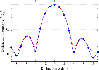
Figure 8: Diffraction intensities of a pure beam of ground state ⁴He₃ at $v=500$ m/s from a $d=100$ nm transmission grating at $\theta^{\prime}=21^{\circ}$ angle of incidence for the grating geometry of Fig. 4. The solid curve was calculated using Eq. (67), the dashed curve shows the two-term cumulant approximation (68). To guide the eye these functions are shown continuously. The circles on top of the solid curve at integer $n$ mark the experimentally accessible diffraction orders $I^{\text{gg}}_{n}/I^{\text{gg}}_{0}$.

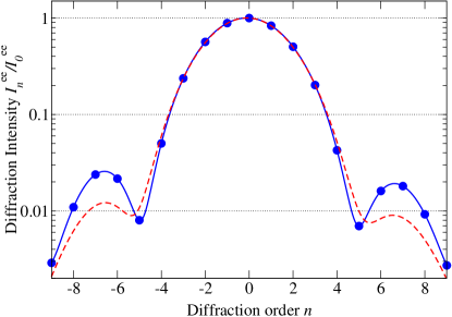
Figure 9: As in Fig. 8 but for a pure beam of excited state ⁴He₃. Due to the larger pair distance of the excited state the effective slit width is smaller, resulting in a considerably wider envelope function than for the ground state.

intensities for a beam of ⁴He₃ in its ground state calculated according to Eqs. (67) and (68). The asymmetry of this diffraction pattern is not as pronounced as in the atom case (Fig. 5). This is due to the threefold mass of the trimer which entails a three times shorter de Broglie wavelength. Similarly, Fig. 9 shows diffraction intensities for a beam of ⁴He₃ in its excited state.

Since inelastic diffraction processes are negligible an experimental diffraction pattern of a ⁴He₃ beam will in general be well described by an incoherent superposition of the individual diffraction patterns of the two bound states weighted by their relative population numbers in the beam. In the following section we first derive the trimer size effect for a pure beam containing trimers in only one state. Hereafter the treatment of a mixed beam will be considered.

VI How to determine the trimer size

VI.1 The trimer size effect

Since the effective slit width of the trimer (69) depends, on the one hand, on the trimer bound state (through $\tau^{\text{tri}}_{{\gamma\gamma}}(\bm{P}^{\prime};S_{2})$) and is, on the other hand, experimentally accessible (through $I_{n}^{\gamma\gamma}$), it represents a link between experiment and theory. Earlier work on atom and dimer diffraction revealed that the difference $S_{0}-S_{\text{eff},\gamma}$ carries information about both the van der Waals surface interaction Grisenti et al. (1999) and the size of weakly bound dimers Grisenti et al. (2000a). The reduction of the slit width by the dimer size was found to be $\frac{1}{2}\left\langle r\right\rangle$ where $\left\langle r\right\rangle$ denotes the dimer bond length. The subsequent evaluation of helium dimer diffraction data yielded the experimental result $\left\langle r\right\rangle=5.2\pm 0.4$ nm for ⁴He₂ Grisenti et al. (2000a).

In the following we derive the corresponding size effect for a trimer. To this end we explicitly insert the trimer transmission function (65) into Eq. (69). By definition the atom transmission functions $\tau^{\text{at}}_{i}(\bm{p}^{\prime}_{i};s_{i2})$ in Eq. (65) are zero if their positional arguments $s_{i2}=r_{i\perp}/\cos(\alpha+\theta^{\prime})$ lie outside the slit interval $[-S_{0}/2,S_{0}/2]$. This fact may be utilized to reduce the integration interval for the center of mass position $S_{2}$: at fixed relative coordinates $\bm{\mathrm{\rho}},\bm{\mathrm{r}}$ the interval may be limited, for $r_{\perp}>0$, to

$$-\frac{S_{0}}{2}+\frac{\Delta^{+}_{2}}{\cos(\alpha+\theta^{\prime})}<S_{2}<\frac{S_{0}}{2}-\frac{\Delta^{+}_{1}}{\cos(\alpha+\theta^{\prime})}$$ (70a)

and, similarly, for $$r_{\perp}<0$$, to

$$-\frac{S_{0}}{2}+\frac{\Delta^{-}_{1}}{\cos(\alpha+\theta^{\prime})}<S_{2}<\frac{S_{0}}{2}-\frac{\Delta^{-}_{2}}{\cos(\alpha+\theta^{\prime})}.$$ (70b)

Here, the geometrical quantities

$$\Delta^{\pm}_{1} =\pm\frac{1}{2}\left\{\frac{m_{2}+m_{3}-m_{1}}{M}\rho_{\perp}+\frac{m_{3}}{m_{2}+m_{3}}r_{\perp}\right.$$

$$\hskip 28.45274pt\left.\pm\left|\rho_{\perp}-\frac{m_{3}}{m_{2}+m_{3}}r_{\perp}\right|\right\}$$ (71)

and

$$\Delta^{\pm}_{2} =\pm\frac{1}{2}\left\{-\frac{m_{2}+m_{3}-m_{1}}{M}\rho_{\perp}+\frac{m_{2}}{m_{2}+m_{3}}r_{\perp}\right.$$

$$\hskip 28.45274pt\left.\pm\left|\rho_{\perp}+\frac{m_{2}}{m_{2}+m_{3}}r_{\perp}\right|\right\}$$ (72)

have been introduced. Neglecting, for the moment, the van der Waals interaction, all atom transmission functions are unity inside the reduced domain of integration (70). In this case the effective slit width depends only on $\Delta^{\pm}_{1}$ and $\Delta^{\pm}_{2}$. Accordingly, we call it the geometrical part of the effective slit width and denote it by

$$S^{\text{geom}}_{\text{eff},\gamma}= S_{0}-\frac{1}{\cos(\alpha+\theta^{\prime})}\text{\,Re\,}\int d^{3}\rho d^{3}r\ |\phi_{\gamma}(\bm{\mathrm{\rho}},\bm{\mathrm{r}})|^{2}$$

$$\times\left\{\left[\Delta^{+}_{1}+\Delta^{+}_{2}\right]\Theta(r_{\perp})+\left[\Delta^{-}_{1}+\Delta^{-}_{2}\right]\Theta(-r_{\perp})\right\}$$ (73)

where $\Theta(r_{\perp})$ is the Heaviside step function. Both integrands in Eq. (73) can be simplified using the transformation properties of the Jacobi coordinates (32) and the wave functions (38). Combining the results, the geometrical part of the effective slit width becomes

$$S^{\text{geom}}_{\text{eff},\gamma}=S_{0}-\frac{\left\langle\left|r^{(23)}_{\perp}\right|\right\rangle_{\gamma}+\left\langle\left|r^{(31)}_{\perp}\right|\right\rangle_{\gamma}+\left\langle\left|r^{(12)}_{\perp}\right|\right\rangle_{\gamma}}{2\cos(\alpha+\theta^{\prime})}$$ (74)

where the expectation values in the numerator are defined as

$$\left\langle\left|r^{(jk)}_{\perp}\right|\right\rangle_{\gamma}=\int d^{3}\rho^{(i)}d^{3}r^{(jk)}\left|\phi_{\gamma}^{(i,jk)}(\bm{\mathrm{\rho}}^{(i)},\bm{\mathrm{r}}^{(jk)})\right|^{2}\left|r^{(jk)}_{\perp}\right|.$$ (75)

In Eq. (74) the symmetric term

$$\frac{1}{2}\left(\left\langle\left|r^{(23)}_{\perp}\right|\right\rangle_{\gamma}+\left\langle\left|r^{(31)}_{\perp}\right|\right\rangle_{\gamma}+\left\langle\left|r^{(12)}_{\perp}\right|\right\rangle_{\gamma}\right)$$ (76)

represents the expectation value of the “width” (projected diameter) of the trimer perpendicular to the incident direction. Therefore, as the factor $[\cos(\alpha+\theta^{\prime})]^{-1}$ corresponds to an orthogonal projection of the perpendicular coordinates onto the slit line (cf. Fig. 10) $S^{\text{geom}}_{\text{eff},\gamma}$ is simply smaller than $S_{0}$ by the projected width of the trimer.

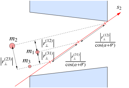
Figure 10: Geometrical interpretation of the effective slit width formula. Clearly, the expression $\frac{1}{2}(|r^{(23)}_{\perp}|+|r^{(31)}_{\perp}|+|r^{(12)}_{\perp}|)$ may be interpreted as the “width” (projected diameter) of the trimer perpendicular to its incident direction. Taking the expectation values with the bound state wave function yields the expression (76). The multiplication by $[\cos(\alpha+\theta^{\prime})]^{-1}$ corresponds to an orthogonal projection onto the slit line $\mathcal{S}$. Hence the slit width $S_{0}$ appears reduced by the projected width of the trimer.

In the presence of the van der Waals interaction an additional term $S^{\text{vdW}}_{\text{eff},\gamma}$ accounting for the deviation from unity of the atom transmission functions arises. The entire effective slit width is the sum

$$S_{\text{eff},\gamma}=S^{\text{geom}}_{\text{eff},\gamma}+S^{\text{vdW}}_{\text{eff},\gamma}.$$ (77)

As the general expression for the van der Waals part $S^{\text{vdW}}_{\text{eff},\gamma}$ is long and little informative we shall not give its general form explicitly.

VI.2 The size effect for three identical Bosons

In the remaining paragraphs of this section we focus on trimers of three identical Bosons, such as the ⁴He₃. By consequence, we denote the masses by $m=m_{i}$ and the equal projected pair distances by $\left\langle|r_{\perp}|\right\rangle_{\gamma}$. The geometric part of the effective slit width (74) immediately reduces to

$$S^{\text{geom}}_{\text{eff},\gamma}=S_{0}-\frac{3}{2}\frac{\left\langle\left|r_{\perp}\right|\right\rangle_{\gamma}}{\cos(\alpha+\theta^{\prime})}.$$ (78)

Moreover, if the spatial extent of the bound state wave function is small compared to the slit width, the van der Waals part $S^{\text{vdW}}_{\text{eff},\gamma}$ is to very good approximation given by

$$S^{\text{vdW}}_{\text{eff},\gamma}\simeq-\text{\,Re\,}\int d^{3}\rho d^{3}r\ |\phi_{\gamma}(\bm{\mathrm{\rho}},\bm{\mathrm{r}})|^{2}$$

$$\left\{\int_{0}^{{S_{0}}/2}dS^{\prime}_{2}\left[1-\tau^{\text{at}}\left(\frac{{\bm{P}}^{\prime}}{3};S^{\prime}_{2}\right)\tau^{\text{at}}\left(\frac{{\bm{P}}^{\prime}}{3};S^{\prime}_{2}-\frac{\left|\rho_{\perp}-\frac{1}{2}|r_{\perp}|\right|}{\cos(\alpha+\theta^{\prime})}\right)\right.\right.$$

$$\left.\left.\ \ \ \times\ \tau^{\text{at}}\left(\frac{{\bm{P}}^{\prime}}{3};S^{\prime}_{2}-\frac{|r_{\perp}|+\left(\rho_{\perp}-\frac{1}{2}|r_{\perp}|\right)\Theta\left(\rho_{\perp}-\frac{1}{2}|r_{\perp}|\right)}{\cos(\alpha+\theta^{\prime})}\right)\right]\right.$$

$$+\!\!\int_{-{S_{0}}/2}^{0}dS^{\prime}_{2}\left.\left[1-\tau^{\text{at}}\left(\frac{{\bm{P}}^{\prime}}{3};S^{\prime}_{2}\right)\tau^{\text{at}}\left(\frac{{\bm{P}}^{\prime}}{3};S^{\prime}_{2}+\frac{\left|\rho_{\perp}+\frac{1}{2}|r_{\perp}|\right|}{\cos(\alpha+\theta^{\prime})}\right)\right.\right.$$

$$\left.\left.\ \ \ \times\ \tau^{\text{at}}\left(\frac{{\bm{P}}^{\prime}}{3};S^{\prime}_{2}+\frac{|r_{\perp}|-\left(\rho_{\perp}+\frac{1}{2}|r_{\perp}|\right)\Theta\left(-\rho_{\perp}-\frac{1}{2}|r_{\perp}|\right)}{\cos(\alpha+\theta^{\prime})}\right)\right]\right\}.$$ (79)

Within the approximation (79) it is evident that $S^{\text{vdW}}_{\text{eff},\gamma}$ is indeed zero if the atom transmission functions are unity inside the slit, and if the spatial extent of the trimer wave function is small on the scale of the slit width. Therefore, if $S^{\text{vdW}}_{\text{eff},\gamma}$ were but a small correction to the full effective slit width (77) it could be neglected, and the projected trimer pair distance $\left\langle|r_{\perp}|\right\rangle$ could be determined using Eq. (78). Experience with dimer diffraction has shown, however, that the effect of the van der Waals interaction can be of the same order as the pair distance Grisenti et al. (2000a) and must be accounted for. Since Eq. (79) depends on the full trimer wave function it cannot be used immediately for the evaluation of experimental data and an approximation is required. The integrand in Eq. (79) is, however, slowly varying on the scale of the variation of $|\phi_{\gamma}(\bm{\mathrm{\rho}},\bm{\mathrm{r}})|^{2}$. Therefore, the positional arguments of the atom transmission functions can approximately be replaced by their expectation values. This approach is in analogy to Ref. Grisenti et al. (2000a). An analysis of the combinations of $\rho_{\perp}$ and $r_{\perp}$, using once more the transformation properties of the relative coordinates (32), shows that these expectation values are expressible solely in terms of $\left\langle|r_{\perp}|\right\rangle$. For example,

$$\left\langle\left|\rho_{\perp}-\frac{1}{2}|r_{\perp}|\right|\right\rangle_{\gamma}=\left\langle\left|r_{\perp}\right|\right\rangle_{\gamma}$$ (80)

and

$$\left\langle\left(\rho_{\perp}-\frac{1}{2}|r_{\perp}|\right)\Theta\left(\rho_{\perp}-\frac{1}{2}|r_{\perp}|\right)\right\rangle_{\gamma}=\frac{1}{4}\left\langle|r_{\perp}|\right\rangle_{\gamma}.$$ (81)

Inserting these one finds as the final form of the van der Waals part of the effective slit width

$$S^{\text{vdW}}_{\text{eff},\gamma}\simeq-\text{\,Re\,}\Bigg{\{}\int_{0}^{{S_{0}}/2}dS^{\prime}_{2}\left[1-\tau^{\text{at}}\left(\frac{{\bm{P}}^{\prime}}{3};S^{\prime}_{2}\right)\right.$$ (82)

$$\times \!\left.\tau^{\text{at}}\left(\frac{{\bm{P}}^{\prime}}{3};S^{\prime}_{2}-\frac{\left\langle|r_{\perp}|\right\rangle_{\gamma}}{\cos(\alpha+\theta^{\prime})}\right)\tau^{\text{at}}\left(\frac{{\bm{P}}^{\prime}}{3};S^{\prime}_{2}-\frac{5}{4}\frac{\left\langle|r_{\perp}|\right\rangle_{\gamma}}{\cos(\alpha+\theta^{\prime})}\right)\right]$$

$$+ \!\int_{-{S_{0}}/2}^{0}dS^{\prime}_{2}\left[1-\tau^{\text{at}}\left(\frac{{\bm{P}}^{\prime}}{3};S^{\prime}_{2}\right)\tau^{\text{at}}\left(\frac{{\bm{P}}^{\prime}}{3};S^{\prime}_{2}+\frac{\left\langle|r_{\perp}|\right\rangle_{\gamma}}{\cos(\alpha+\theta^{\prime})}\right)\right.$$

$$\times \!\left.\tau^{\text{at}}\left(\frac{{\bm{P}}^{\prime}}{3};S^{\prime}_{2}+\frac{5}{4}\frac{\left\langle|r_{\perp}|\right\rangle_{\gamma}}{\cos(\alpha+\theta^{\prime})}\right)\right]\Bigg{\}}.$$

In order to test the validity of this approximation we carried out a numerical analysis of the error introduced by the replacement of Eq. (79) by Eq. (82): if applied to experimental data the approximation entails, for the two theoretically predicted bound states of ⁴He₃, a systematic overestimation of $\left\langle|r_{\perp}|\right\rangle$ by 7% (⁴He₃ ground state), or 3% (excited state). As seen from Fig. 11 the approximation is more reliable at high velocities as the impact of the van der Waals interaction becomes smaller.

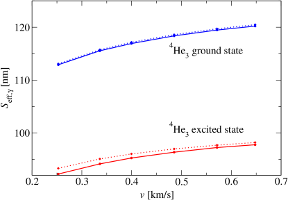
Figure 11: Effective slit widths versus the beam velocity $v=|\bm{\mathrm{P}}^{\prime}|/M$ for the ground state and the excited state of ⁴He₃. The numerical results using the full expression Eq. (79) are shown as solid curves and the approximation Eq. (82) as dotted curves. The angle of incidence was taken as $\theta^{\prime}=21^{\circ}$. The approximation becomes more reliable at high velocities as the impact of the van der Waals interaction decreases. Asymptotically, for high velocities, both pairs of curves approach their respective upper limits $S^{\text{geom}}_{\text{eff},\gamma}$ given by Eq. (78).

Theoretical studies of the helium trimer commonly state the expectation value of the pair distance $\left\langle r\right\rangle$ itself, where $r=|\bm{\mathrm{r}}|$, rather than a component such as $\left\langle|r_{\perp}|\right\rangle$. To link experimental results to these, a relation between $\left\langle r\right\rangle$ and $\left\langle|r_{\perp}|\right\rangle$ must be established. Both predicted ⁴He₃ bound states are spherically symmetric (zero total angular momentum). Moreover, the two-body scattering matrix corresponding to the He-He potential is dominated by the shallow $s$-wave bound state pole of ⁴He₂, and higher partial waves may to good approximation be neglected Nakaichi-Maeda and Lim (1983). By the Faddeev equations (e.g. Ref. Sitenko (1971)) for the helium trimer bound state, it is then possible to derive the relation

$$\left\langle|r_{\perp}|\right\rangle=\frac{1}{2}\left\langle r\right\rangle.$$ (83)

In summary, the effective slit width (77) depends to good approximation only on one trimer parameter, namely the expectation value of the pair distance $\left\langle r\right\rangle$. Consequently, $\left\langle r\right\rangle$ can, in principle, be determined from trimer diffraction data.

VI.3 Experimental considerations

Using the results of the preceding sections the improvement in resolution through diffraction at non-normal incidence over normal incidence may be estimated. The evaluation process of experimental data involves two main steps: Firstly, values for the effective slit width $S_{\text{eff},\gamma}$ must be obtained by numerical fits of the intensity formula (68) to experimental diffraction patterns. Secondly, $\left\langle r\right\rangle$ is determined from a fit of Eq. (77) to the values for $S_{\text{eff},\gamma}$. The stronger the dependence of this procedure on $\left\langle r\right\rangle$ the more precisely $\left\langle r\right\rangle$ can be determined. As $\left\langle r\right\rangle$ changes the width of the Kirchhoff-like slit function in Eq. (68) a natural measure for this dependence is provided by the number of diffraction orders under the central maximum of the slit function to either side of the forward direction. This number, which we denote here by $n_{c}$, and which we treat as a continuous variable, can be approximately written as

$$n_{c}=\frac{d_{\perp}}{s_{\perp}}$$ (84)

where $d_{\perp}$ denotes the (projected) period perpendicular to the beam and $s_{\perp}$ denotes the projected slit width. At the angle of incidence $\theta^{\prime}$ the projected period is $d_{\perp}=d\cos\theta^{\prime}$. Furthermore, neglecting for this estimate the van der Waals part, we insert $s_{\perp}=S^{\text{geom}}_{\text{eff},\gamma}\cos(\alpha+\theta^{\prime})$ for the projected slit width of the deep grating where $S^{\text{geom}}_{\text{eff},\gamma}$ will be taken from Eq. (78). The relative variation of $n_{c}$ with $\left\langle r\right\rangle$ can then be calculated and becomes, to leading order in $\left\langle r\right\rangle/S_{0}$,

$$\frac{1}{n_{c}}{\frac{\text{d}n_{c}}{\text{d}\left\langle r\right\rangle}}\simeq\frac{3}{4}\frac{1}{S_{0}\cos(\alpha+\theta^{\prime})}.$$

In contrast, at normal incidence the right hand side would be $3/(4s_{0})$. Inserting the parameters of Fig. 8 yields $(\text{d}n_{c}/\text{d}\left\langle r\right\rangle)/n_{c}\approx 2.6\times 10^{-2}\,\text{nm}^{-1}$ for $\theta^{\prime}=21^{\circ}$ as compared to $1.2\times 10^{-2}\,\text{nm}^{-1}$ for normal incidence. This roughly twofold gain in sensitivity is expected to halve the final error bars on $\left\langle r\right\rangle$.

Finally, since the population ratio of the two predicted ⁴He₃ states in the nozzle beam is generally unknown the situation of a mixed beam must be considered. To analyze this we have summed diffraction patterns as shown in Figs. 8 and 9 for different population ratios. Hereafter, we have used Eq. (68) to determine, from the summed patterns, an average effective slit width $S_{\text{eff}}$ and from this an average bond length $\left\langle r\right\rangle$. It turned out that the such determined $\left\langle r\right\rangle$ varies almost linearly with the population ratio from the ground state value of $\left\langle r\right\rangle$ (pure ground state beam) to the excited state value (pure excited state beam). Therefore, three possible outcomes of an experiment are to be expected. A value of $\left\langle r\right\rangle\approx 1$ nm would be attributed to the ground state and indicate a negligible (or zero) population of the excited state. Equivalently, a result of about $8$ nm would doubtlessly provide evidence for the excited state and its large pair distance. Thirdly, a value in between these two would indicate that both states are present and evidence for the excited state would still be available. A controlled variation of the accessible beam parameters might then allow to influence the population ratio in favor of either state and to measure the pair distance for one state with less disturbance by the other.

VII Conclusions

Motivated by the long-standing interest in the Efimov effect Efimov (1970) we have studied the diffraction of weakly bound trimers in a typical matter optics setup. As an earlier diffraction experiment for the spatially extended helium dimer ($\left\langle r\right\rangle=5.2$ nm) Grisenti et al. (2000a) had indicated that the resolution provided by a custom $s_{0}=60$ nm transmission grating, at normal incidence, may be insufficient to resolve the helium trimer ground state ($\left\langle r\right\rangle=0.96$ nm predicted Barletta and Kievsky (2001)) it had suggested itself to use oblique (non-normal) incidence at a rotated transmission grating for reducing the projected slit width. The partial shadowing of the slits caused by the finite thickness of the etched material grating has required, however, a revision of the theory of atom diffraction. In particular, the familiar mirror symmetry encountered in diffraction patterns from normal incidence is lifted for non-normal incidence. This effect was visible in Fig. 5 of Ref. Grisenti et al. (2000b) but went unnoticed. It has been traced back to the non-alignment of the direction of periodicity of the grating with the shadow lines of its bars, or, equivalently, its slit lines. The weak attractive van der Waals surface interaction, which introduces an additional but minor asymmetry, has been taken into account in a way similar to the case of normal incidence.

Using atom diffraction as one building block, the multi-channel many-body quantum mechanical scattering theory approach of Refs. Hegerfeldt and Köhler (1998); Hegerfeldt and Köhler (2000a) has been extended to derive the constitutive formulas of trimer diffraction. While this procedure structurally partly parallels that of dimer diffraction it is mathematically more complex due to the additional atom. The resulting equations for the trimer diffraction pattern, however, have been readily interpretable and provide intuitive physical insight into diffraction of weakly bound molecules: the significant measurable quantity is the quantum mechanical expectation value of the “width” (projected diameter) of the trimer perpendicular to its flight direction. For identical Boson trimers, such as the helium trimer, the width is related to the molecular bond length by $\frac{3}{4}\left\langle r\right\rangle$. This fact can be used, in principle, to determine $\left\langle r\right\rangle$ from a matter diffraction experiment.

If a transmission grating of the type used earlier by Grisenti et al Grisenti et al. (1999) is rotated by $\theta^{\prime}=21^{\circ}$ the projected slits appear approximately half as wide as the nominal slits of the grating. This leads to an estimated doubling of the resolution, sufficient to determine the ground state pair distance of ⁴He₃. Moreover, should the ⁴He₃ Efimov state, whose pair distance is predicted to be larger by almost an order of magnitude Barletta and Kievsky (2001), exist and should its population in the beam be significant, it ought to be clearly distinguishable from the ground state solely by its size.

Appendix A Surface interaction

Earlier work has shown that at beam velocities typically encountered in matter diffraction experiments the effective reduction of the slit width due to both the van der Waals surface interaction and the finite molecular size can be of the same order of magnitude Grisenti et al. (1999); Grisenti et al. (2000a). A quantitative determination of the atom transmission function $\tau^{\text{at}}(\bm{p}^{\prime};s_{2})$, which was inserted into Eq. (16), is therefore necessary. As in Ref. Grisenti et al. (1999) we use the eikonal approximation to write $\tau^{\text{at}}(\bm{p}^{\prime};s_{2})=\exp[i\varphi(\bm{p}^{\prime};s_{2})]$ for $s_{2}$ inside the slit, and $\tau^{\text{at}}(\bm{p}^{\prime};s_{2})=0$ outside. The phase function $\varphi(\bm{p}^{\prime};s_{2})$ is given by Joachain (1975)

$$\varphi(\bm{p}^{\prime};s_{2})=-(\hbar v)^{-1}\int dt\ W_{\text{surf}}(\bm{s}(t)),\quad v=\frac{|\bm{p}^{\prime}|}{m},$$ (85)

where the straight path of integration $\bm{s}(t)$ must be taken to run parallel to the direction of incidence, and to cross the slit line $\mathcal{S}$ at the position $s_{2}$. The surface interaction $W_{\text{surf}}(\bm{x})$ at a position $\bm{x}$ between two bars is calculated from the integration of an attractive $-C_{6}/l^{6}$ potential of Lennard-Jones type (the repulsive part has already been modeled by the boundary conditions in Sec. II) over the volume of the bars. Carrying out all four integrations for the typical wedge-shaped bars shown in Fig. 4 the phase function can be calculated explicitly. Using the abbreviations

$$C_{3}=\frac{\pi C_{6}}{6},\quad\widetilde{d}=\frac{\cos\theta^{\prime}}{\cos(\alpha+\theta^{\prime})}d,\quad\widetilde{s_{0}}=\frac{\cos\theta^{\prime}}{\cos(\alpha+\theta^{\prime})}s_{0},$$

it reads

$$\varphi(\bm{p}^{\prime};s_{2})=\frac{C_{3}}{2\hbar v\cos^{2}\theta^{\prime}\cos^{2}(\alpha+\theta^{\prime})}$$

$$\times \left\{\frac{\xi_{11}^{-2}+(\xi_{11}-\widetilde{d})^{-2}-\xi_{12}^{-2}-(\xi_{12}+\widetilde{d})^{-2}}{\tan\theta^{\prime}+\tan\beta}\right.$$

$$\left.+\frac{\xi_{21}^{-2}+(\xi_{21}-\widetilde{d})^{-2}-\xi_{22}^{-2}-(\xi_{22}-\widetilde{d})^{-2}}{\tan\theta^{\prime}-\tan\beta}\right\}$$

where $\xi_{11}=\frac{S_{0}}{2}-s_{2}$, $\xi_{21}=\frac{S_{0}}{2}+s_{2}$, $\xi_{12}=\frac{S_{0}}{2}-s_{2}-\widetilde{s_{0}}+\frac{\cos((\alpha+\theta^{\prime})-2\theta^{\prime})}{\cos(\alpha+\theta^{\prime})}S_{0}$, and $\xi_{22}=\frac{S_{0}}{2}-s_{2}-\widetilde{s_{0}}$.

References

- Luo et al. (1995) F. Luo, C. F. Giese, and W. R. Gentry, J. Chem. Phys. 104, 1151 (1995).
- Schöllkopf and Toennies (1994) W. Schöllkopf and J. P. Toennies, Science 266, 1345 (1994).
- Grisenti et al. (2000a) R. E. Grisenti, W. Schöllkopf, J. P. Toennies, G. C. Hegerfeldt, T. Köhler, and M. Stoll, Phys. Rev. Lett. 85, 2284 (2000a).
- Barletta and Kievsky (2001) P. Barletta and A. Kievsky, Phys. Rev. A 64, 042514 (2001).
- Lim et al. (1977) T. K. Lim, S. K. Duffy, and W. C. Damert, Phys. Rev. Lett. 38, 341 (1977).
- Esry et al. (1996) B. D. Esry, C. D. Lin, and C. H. Greene, Phys. Rev. A 54, 394 (1996).
- (7) Recently, several groups working in the field of ultra-cold molecules demonstrated a controlled variation of the scattering length in alkali atom interactions over a wide range of negative and positive values through a Feshbach resonance. This raises the hope to demonstrate the Efimov effect under these unusual conditions. For references see, for example, E. A. Donley et al, Nature 417, 529 (2002), and J. Herbig et al, Science 301, 1510 (2003)
- Keith et al. (1988) D. W. Keith, M. L. Schattenburg, H. I. Smith, and D. E. Pritchard, Phys. Rev. Lett. 61, 1580 (1988).
- Carnal and Mlynek (1991) O. Carnal and J. Mlynek, Phys. Rev. Lett. 66, 2689 (1991).
- Shimizu et al. (1992) F. Shimizu, K. Shimizu, and H. Takuma, Phys. Rev. A 46, R17 (1992).
- Savas et al. (1995) T. A. Savas, S. N. Shah, J. M. Carter, and H. I. Smith, J. Vac. Sci. Technol. B 13, 2732 (1995).
- Grisenti et al. (1999) R. E. Grisenti, W. Schöllkopf, J. P. Toennies, G. C. Hegerfeldt, and T. Köhler, Phys. Rev. Lett. 83, 1755 (1999).
- Hornberger et al. (2003) K. Hornberger, S. Uttenthaler, B. Brezger, L. Hackermüller, M. Arndt, and A. Zeilinger, Phys. Rev. Lett. 90, 160401 (2003).
- Arndt et al. (1999) M. Arndt, O. Nairz, J. Vos-Andreae, C. Keller, G. van der Zouw, and A. Zeilinger, Nature (London) 401, 680 (1999).
- Hegerfeldt and Köhler (2000a) G. C. Hegerfeldt and T. Köhler, Phys. Rev. A 61, 23606 (2000a).
- Hegerfeldt and Köhler (1998) G. C. Hegerfeldt and T. Köhler, Phys. Rev. A 57, 2021 (1998).
- Brühl et al. (2002) R. Brühl, P. Fouquet, R. E. Grisenti, J. P. Toennies, G. C. Hegerfeldt, T. Köhler, M. Stoll, and C. Walter, Europhys. Lett. 59, 357 (2002).
- Janzen and Aziz (1995) A. R. Janzen and R. A. Aziz, J. Chem. Phys. 103, 9626 (1995).
- Gdanitz (2001) R. J. Gdanitz, Mol. Phys. 99, 923 (2001).
- Huber and Lim (1977) H. S. Huber and T. K. Lim, J. Chem. Phys. 68, 1006 (1977).
- Nakaichi-Maeda and Lim (1983) S. Nakaichi-Maeda and T. K. Lim, Phys. Rev. A 28, 692 (1983).
- Fedorov and Jensen (1993) D. V. Fedorov and A. S. Jensen, Phys. Rev. Lett. 71, 4103 (1993).
- Nielsen et al. (1998) E. Nielsen, D. V. Fedorov, and A. S. Jensen, J. Phys. B 31, 4085 (1998).
- Motovilov et al. (1997) A. K. Motovilov, S. A. Sofianos, and E. A. Kolganova, Chem. Phys. Lett. 275, 168 (1997).
- Kolganova et al. (1998) E. A. Kolganova, A. K. Motovilov, and S. A. Sofianos, J. Phys. B 31, 1279 (1998).
- Roudnev and Yakovlev (2000) V. Roudnev and S. Yakovlev, Chem. Phys. Lett. 328, 97 (2000).
- Motovilov et al. (2001) A. K. Motovilov, W. Sandhas, S. A. Sofianos, and E. A. Kolganova, Eur. Phys. J. D 13, 33 (2001).
- Bruch (1999) L. W. Bruch, J. Chem. Phys. 110, 2410 (1999).
- Lewerenz (1997) M. Lewerenz, J. Chem. Phys. 106, 4596 (1997).
- Røeggen and Almlöf (1995) I. Røeggen and J. Almlöf, J. Chem. Phys. 102, 7095 (1995).
- Efimov (1970) V. Efimov, Phys. Lett. 33B, 563 (1970). Comments Nucl. Part. Phys 19, 271 (1990).
- Bruch et al. (2002) L. W. Bruch, W. Schöllkopf, and J. P. Toennies, J. Chem. Phys. 117, 1544 (2002).
- Born and Wolf (1959) M. Born and E. Wolf, Principles of Optics (Pergamon Press, London, 1959), §11.3.
- (34) Since one may replace by in Eq. (III.1).
- Grisenti et al. (2000b) R. E. Grisenti, W. Schöllkopf, J. P. Toennies, J. R. Manson, T. A. Savas, and H. I. Smith, Phys. Rev. A 61, 033608 (2000b).
- Lennard-Jones (1932) J. E. Lennard-Jones, Trans. Faraday Soc. 28, 334 (1932).
- Raskin and Kusch (1969) D. Raskin and P. Kusch, Phys. Rev. 179, 712 (1969).
- Newton (1966) R. G. Newton, Scattering Theory of Waves and Particles (McGraw-Hill, 1966).
- Morse and Feshbach (1953) P. M. Morse and H. Feshbach, Methods of Theoretical Physics (McGraw-Hill, New York, 1953), §11.4, p. 1551.
- Colton and Kress (1983) D. Colton and R. Kress, Integral equation methods in scattering theory (John Wiley & Sons, Inc., 1983).
- Abramowitz and (Hg.) M. Abramowitz and I. A. S. (Hg.), Handbook of Mathematical Functions (Dover Publications, 1968).
- (42) The theory of trimer diffraction derived in Sections IV and V also applies if one or more of the atoms are substituted by a more strongly bound molecule. In the Ar2–HCl cluster, for example, the binding between the hydrogen and the chlorine atom is comparatively tight Klots et al. (1987). It is however required that electronic or rovibrational excitations of the molecule cannot occur at the energies available in a nozzle beam (a few tens of meV).
- Klots et al. (1987) T. D. Klots, C. Chuang, R. S. Ruoff, T. Emilsson, and H. S. Gutowsky, J. Chem. Phys. 86, 5315 (1987).
- Faddeev (1961) L. D. Faddeev, Soviet Phys. - JETP 12, 1014 (1961).
- Sitenko (1971) A. G. Sitenko, Lectures in Scattering Theory (Pergamon Press, 1971).
- Lovelace (1964) C. Lovelace, Phys. Rev. 135, B 1225 (1964).
- Tang et al. (1995) K. T. Tang, J. P. Toennies, and C. L. Yiu, Phys. Rev. Lett. 74, 1546 (1995).
- Braaten and Hammer (2003) E. Braaten and H.-W. Hammer, Phys. Rev. A 67, 042706 (2003).
- Braaten et al. (2003) E. Braaten, H.-W. Hammer, and M. Kusunoki, Phys. Rev. A 67, 022505 (2003).
- Yamashita et al. (2003) M. T. Yamashita, R. S. M. de Carvalho, L. Tomio, and T. Frederico, Phys. Rev. A 68, 012506 (2003).
- Hegerfeldt and Köhler (2000b) G. C. Hegerfeldt and T. Köhler, Phys. Rev. Lett. 84, 3215 (2000b).
- Alt et al. (1967) E. O. Alt, P. Grassberger, and W. Sandhas, Nucl. Phys. B 2, 167 (1967).
- Glöckle (1983) W. Glöckle, The Quantum Mechanical Few-Body Problem (Springer, Berlin, 1983).
- Stoll and Köhler (2002) M. Stoll and T. Köhler, J. Phys. B 35, 4999 (2002).
- Joachain (1975) C. J. Joachain, Quantum Collision Theory (North-Holland Physics Publishing, 1975).