Collapse models: analysis of the free particle dynamics

Abstract

We study a model of spontaneous wavefunction collapse for a free quantum particle. We analyze in detail the time evolution of the single–Gaussian solution and the double–Gaussian solution, showing how the reduction mechanism induces the localization of the wavefunction in space; we also study the asymptotic behavior of the general solution. With an appropriate choice for the parameter $\lambda$ which sets the strength of the collapse mechanism, we prove that: i) the effects of the reducing terms on the dynamics of microscopic systems are negligible, the physical predictions of the model being very close to those of standard quantum mechanics; ii) at the macroscopic scale, the model reproduces classical mechanics: the wavefunction of the center of mass of a macro–object behaves, with high accuracy, like a point moving in space according to Newton’s laws.

I Introduction

Models of spontaneous wavefunction collapse grw1 ; grw2 ; grw6 ; pp1 ; di1 ; di3 ; bel1 ; bel2 ; bla1 ; jp1 ; jp2 ; ip ; ad1 ; ad2 ; bar1 have reached significant results in providing a solution to the measurement problem of quantum mechanics. This goal is achieved by modifying the Schrödinger equation, adding appropriate non–linear stochastic terms: such terms do not modify appreciably the standard quantum dynamics of microscopic systems; at the same time, they rapidly reduce the superposition of two or more macroscopically different states of a macro–object into one of them; in particular, they guarantee that measurements made on microscopic systems always have definite outcomes, and with the correct quantum probabilities. In this way, collapse models describe — within one single dynamical framework — both the quantum properties of microscopic systems and the classical properties of macroscopic objects, providing a unified description of micro– and macro–phenomena.

In this paper, we investigate the physical properties of a collapse model describing the (one–dimensional) evolution of a free quantum particle subject to spontaneous localizations in space; its dynamics is governed by the following stochastic differential equation in the Hilbert space $L^{2}({\mathbb{R}})$:

$$d\,\psi_{t}(x) = \left[-\frac{i}{\hbar}\,\frac{p^{2}}{2m}\,dt+\sqrt{\lambda}\,(q-\langle q\rangle_{t})\,dW_{t}\right.$$ (1)

$$\left.-\frac{\lambda}{2}\,(q-\langle q\rangle_{t})^{2}dt\right]\psi_{t}(x),$$

where $q$ and $p$ are the position and momentum operators, respectively, and $\langle q\rangle_{t}\equiv\langle\psi_{t}|q|\psi_{t}\rangle$ denotes the quantum average of the operator $q$; $m$ is the mass of the particle, while $\lambda$ is a positive constant which sets the strength of the collapse mechanism. The stochastic dynamics is governed by a standard Wiener process $W_{t}$, defined on the probability space $(\Omega,{\mathcal{F}},{\mathbb{P}})$ with the natural filtration $\{{\mathcal{F}}_{t}:t\geq 0\}$ defined on it.

The value of the collapse constant $\lambda$ is given by the formula:

$$\lambda\;=\;\frac{m}{m_{0}}\,\lambda_{0},$$ (2)

where $m_{0}$ is a reference mass which we choose to be equal to that of a nucleon, and $\lambda_{0}$ is a fixed constant which we take equal to:

$$\lambda_{0}\;\simeq\;10^{-2}\,\makebox{m${}^{-2}$ sec${}^{-1}$};$$ (3)

this value corresponds to the product of the two parameters $\Lambda_{\makebox{\tiny GRW}}$ and $\alpha_{\makebox{\tiny GRW}}$ of the GRW collapse–model grw1 , where $\Lambda_{\makebox{\tiny GRW}}\simeq 10^{-16}$ sec^-1 is the localization rate for a nucleon and $1/\sqrt{\alpha_{\makebox{\tiny GRW}}}\simeq 10^{-7}$ m is the width of the Gaussian wavefunction inducing the localizations.

Eq. (1) has already been subject to investigation: in ref jp1 a theorem proves the existence and uniqueness of strong solutions; in refs jp1 ; di1 ; bel2 ; hal some properties of the solutions have been analyzed: in particular, it has been shown that Gaussian wavefunctions are solutions of Eq. (1), that their spread reaches an asymptotic finite value (we speak in this case of a “stationary” solution), and that the general solution reaches asymptotically a stationary Gaussian solution. Finally, in ref di3 , Eq. (1) has been first proposed as a universal model of wavefunction collapse.

The aim of our work is to provide a detailed analysis of the physical properties of the solutions of Eq. (1). After some mathematical preliminaries (Sec. II), we will study the time evolution of the two most interesting types of wavefunctions: the single–Gaussian (Sec. III) and the double–Gaussian wavefunctions (Sec. IV); in Sec. V we will discuss the asymptotic behavior of the general solution.

We will next study the effects of the stochastic dynamics on microscopic systems (Sec. VI) and on macroscopic objects (Sec. VII); in the first case, we will see that the prediction of the model are very close to those of standard quantum mechanics, while in the second case we will show that the wavefunction of a macro–object is well localized in space and behaves like a point moving in space according to the classical laws of motion. We end up with some concluding remarks (Sec. VIII).

II Linear Vs Non Linear Equation

The easiest way to find solutions of a non–linear equation is — when feasible — to linearize it: this is possible for Eq. (1) and the procedure is well known in the literature grw2 ; grw6 ; jp1 ; bar1 ; bar3 ; hol1 . Let us consider the following linear stochastic differential equation:

$$d\,\phi_{t}(x)\;=\;\left[-\frac{i}{\hbar}\,\frac{p^{2}}{2m}\,dt+\sqrt{\lambda}\,q\,d\xi_{t}-\frac{\lambda}{2}\,q^{2}dt\right]\phi_{t}(x);$$ (4)

$\xi_{t}$ is a standard Wiener process defined on the probability space $(\Omega,{\mathcal{F}},{\mathbb{Q}})$, where ${\mathbb{Q}}$ is a new probability measure, whose connection with ${\mathbb{P}}$ will be clear in what follows. Contrary to Eq. (1), the above equation does not preserve the norm of statevectors, so let us define the normalized vectors:

$$\psi_{t}\;=\;\left\{\begin{array}[]{cl}\phi_{t}/\|\phi_{t}\|&\makebox{if: $\|\phi_{t}\|\neq 0$,}\\ \makebox{a fixed unit vector}&\makebox{if: $\|\phi_{t}\|=0$.}\end{array}\right.$$ (5)

By using Itô calculus, it is not difficult to show that $\psi_{t}$ defined by (5) is a solution of Eq. (1), whenever $\phi_{t}$ solves Eq. (4). We now briefly explain the relations between the two probability measures ${\mathbb{Q}}$ and ${\mathbb{P}}$, and between the two Wiener processes $\xi_{t}$ and $W_{t}$.

The key property of Eq. (4) is that $p_{t}\equiv\|\phi_{t}\|^{2}$ is a martingale jp1 ; hol1 satisfying the following stochastic differential equation:

$$dp_{t}\;=\;2\sqrt{\lambda}\,\langle q\rangle_{t}\,p_{t}\,d\xi_{t},$$ (6)

with $\langle q\rangle_{t}=\langle\psi_{t}|q|\psi_{t}\rangle$. As a consequence of the martingale property (and assuming, as we shall always do, that $\|\phi_{0}\|=1$) $p_{t}$ can be used to generate a new probability measure $\tilde{\mathbb{P}}$ on $(\Omega,{\mathcal{F}})$ barr ; we choose ${\mathbb{Q}}$ in such a way that the new measure $\tilde{\mathbb{P}}$ coincides with ${\mathbb{P}}$.

Given this, Girsanov’s theorem ls provides a simple relation between the Wiener process $\xi_{t}$ defined on $(\Omega,{\mathcal{F}},{\mathbb{Q}})$, and the Wiener process $W_{t}$ defined on $(\Omega,{\mathcal{F}},{\mathbb{P}})$:

$$W_{t}\;=\;\xi_{t}-2\sqrt{\lambda}\int_{0}^{t}\langle q\rangle_{s}\,ds.$$ (7)

The above results imply that one can find the solution $\psi_{t}$ of Eq. (1), given the initial condition $\psi_{0}$, by using the following procedure:

1. Find the solution $\phi_{t}$ of Eq. (4), with the initial condition $\phi_{0}=\psi_{0}$.

2. Normalize the solution: $\phi_{t}\rightarrow\psi_{t}=\phi_{t}/\|\phi_{t}\|$.

3. Make the substitution: $d\xi_{t}\rightarrow dW_{t}+2\sqrt{\lambda}\langle q\rangle_{t}$.

The advantage of such an approach is that one can exploit the linear character of Eq. (4) to analyze the properties of the nonlinear Eq. (1); as we shall see, the difficult part will be computing $\langle q\rangle_{t}$ from $\phi_{t}$ (step 3): this is where non linearity enters in a non–trivial way.

III Single Gaussian solution

We start our analysis by taking, as a solution, a single–Gaussian wavefunction:

$$\phi_{t}^{\makebox{\tiny S}}(x)=\makebox{exp}\left[-a_{t}(x-\overline{x}_{t})^{2}+i\overline{k}_{t}x+\gamma_{t}\right],$$ (8)

where $a_{t}$ and $\gamma_{t}$ are supposed to be complex functions of time, while $\overline{x}_{t}$ and $\overline{k}_{t}$ are taken to be real. By inserting (8) into Eq. (4), one finds the following sets of stochastic differential equations:

$$da_{t} = \left[\lambda-\frac{2i\hbar}{m}\left(a_{t}\right)^{2}\right]dt$$ (9)

$$d\overline{x}_{t} = \frac{\hbar}{m}\,\overline{k}_{t}\,dt+\frac{\sqrt{\lambda}}{2a_{t}^{\makebox{\tiny R}}}\left[d{\xi}_{t}-2\sqrt{\lambda}\overline{x}_{t}\,dt\right]$$ (10)

$$d\overline{k}_{t} = -\sqrt{\lambda}\,\frac{a_{t}^{\makebox{\tiny I}}}{a_{t}^{\makebox{\tiny R}}}\left[d{\xi}_{t}-2\sqrt{\lambda}\overline{x}_{t}\,dt\right]$$ (11)

$$d\gamma_{t}^{\makebox{\tiny R}} = \left[\lambda\overline{x}^{2}_{t}+\frac{\hbar}{m}a_{t}^{\makebox{\tiny I}}\right]dt+\sqrt{\lambda}\overline{x}_{t}\left[d{\xi}_{t}-2\sqrt{\lambda}\overline{x}_{t}\,dt\right]$$ (12)

$$d\gamma_{t}^{\makebox{\tiny I}} = \left[-\frac{\hbar}{m}a_{t}^{\makebox{\tiny R}}-\frac{\hbar}{2m}\overline{k}^{2}_{t}\right]dt$$ (13)

$$+\sqrt{\lambda}\,\frac{a_{t}^{\makebox{\tiny I}}}{a_{t}^{\makebox{\tiny R}}}\,\overline{x}_{t}\left[d{\xi}_{t}-2\sqrt{\lambda}\overline{x}_{t}\,dt\right].$$

For a single–Gaussian wavefunction, the two equations for $\gamma_{t}$ can be omitted since the real part of $\gamma_{t}$ is absorbed into the normalization factor, while the imaginary part gives an irrelevant global fase.

The normalization procedure is trivial, and also the Girsanov transformation (7) is easy since, for a Gaussian wavefunction like (8), one simply has $\langle q\rangle_{t}=\overline{x}_{t}$. We then have the following set of stochastic differential equations for the relevant parameters:

$$da_{t} = \left[\lambda-\frac{2i\hbar}{m}\,\left(a_{t}\right)^{2}\right]dt,$$ (14)

$$d\overline{x}_{t} = \frac{\hbar}{m}\,\overline{k}_{t}\,dt+\frac{\sqrt{\lambda}}{2a_{t}^{\makebox{\tiny R}}}\,dW_{t},$$ (15)

$$d\overline{k}_{t} = -\sqrt{\lambda}\,\,\frac{a_{t}^{\makebox{\tiny I}}}{a_{t}^{\makebox{\tiny R}}}\,dW_{t};$$ (16)

throughout this section, we will discuss the physical implications of these equations.

III.1 The equation for $a_{t}$

Eq. (14) for $a_{t}$ can be easily solved bel2 ; jp1 :

$$a_{t}\;=\;c\tanh\left[b\,t+k\right],$$ (17)

with:

$$c = (1-i)\frac{1}{2}\sqrt{\frac{m\lambda}{\hbar}},\quad b=(1+i)\sqrt{\frac{\hbar\lambda}{m}},$$

$$k = \tanh^{-1}\left[\frac{a_{0}}{c}\right].$$ (18)

After some algebra, one obtains the following analytical expressions for the real and the imaginary parts of $a_{t}$:

$$a_{t}^{\makebox{\tiny R}} = \;\;\;\frac{\lambda}{\omega}\,\,\frac{\sinh(\omega t+\varphi_{1})+\sin(\omega t+\varphi_{2})}{\cosh(\omega t+\varphi_{1})+\cos(\omega t+\varphi_{2})},\qquad{}$$ (19)

$$a_{t}^{\makebox{\tiny I}} = -\frac{\lambda}{\omega}\,\,\frac{\sinh(\omega t+\varphi_{1})-\sin(\omega t+\varphi_{2})}{\cosh(\omega t+\varphi_{1})+\cos(\omega t+\varphi_{2})},\quad$$ (20)

where we have defined the frequency:

$$\omega\;=\;2\,\sqrt{\frac{\hbar\lambda_{0}}{m_{0}}}\;\simeq\;10^{-5}\;\makebox{sec${}^{-1}$},$$ (21)

which does not depend on the mass of the particle. The two parameters $\varphi_{1}$ and $\varphi_{2}$ are functions of the initial condition: $\varphi_{1}=2k^{\makebox{\tiny R}}$, $\varphi_{2}=2k^{\makebox{\tiny I}}$.

An important property of $a_{t}^{\makebox{\tiny R}}$ is positivity:

$$a_{0}^{\makebox{\tiny R}}>0\quad\longrightarrow\quad a_{t}^{\makebox{\tiny R}}>0\qquad\forall\;t>0,$$ (22)

which guarantees that an initially Gaussian wavefunction does not diverge at any later time. To prove this, we first note that the denominator of (19) cannot be negative; if it is equal to zero then also the numerator is zero: this discontinuity can be removed by using expression (17) for $a_{t}$, which — according to the values (III.1) for $b$ and $k$ — is analytic for any $t$. It is then sufficient to show that the numerator remains positive throughout time. Let us consider the function $f(t)=\sinh(\omega t+\varphi_{1})+\sin(\omega t+\varphi_{2})$; we have that $f(0)>0$ and $f^{\prime}(t)\geq 0$ for any $t$, which implies that $f(t)>0$ for any $t$, as desired. Note that positivity of $a_{t}^{\makebox{\tiny R}}$ matches with the fact that Eq. (1) preserves the norm of statevectors.

III.2 The spread in position and momentum

The time evolution of the spread in position and momentum of the Gaussian wavefunction (8),

$$\sigma_{q}(t) = \sqrt{\langle q^{2}\rangle-\langle q\rangle^{2}}\;=\;\frac{1}{2}\sqrt{\frac{1}{a_{t}^{\makebox{\tiny R}}}},$$

$$\sigma_{p}(t) = \sqrt{\langle p^{2}\rangle-\langle p\rangle^{2}}\;=\;\hbar\,\sqrt{\frac{(a_{t}^{\makebox{\tiny R}})^{2}+(a_{t}^{\makebox{\tiny I}})^{2}}{a_{t}^{\makebox{\tiny R}}}},$$ (23)

is given by the following analytical expressions:

$$\sigma_{q}(t) = \sqrt{\frac{\hbar}{m\omega}}\,\sqrt{\frac{\cosh(\omega t+\varphi_{1})+\cos(\omega t+\varphi_{2})}{\sinh(\omega t+\varphi_{1})+\sin(\omega t+\varphi_{2})}},$$ (24)

$$\sigma_{p}(t) = \sqrt{\frac{\hbar m\omega}{2}}\,\sqrt{\frac{\cosh(\omega t+\varphi_{1})-\cos(\omega t+\varphi_{2})}{\sinh(\omega t+\varphi_{1})+\sin(\omega t+\varphi_{2})}}.\;\;\;\;\;$$ (25)

Fig. 1 shows the different time dependence of the spread in position, as given by the Schrödinger equation and by the stochastic equation:

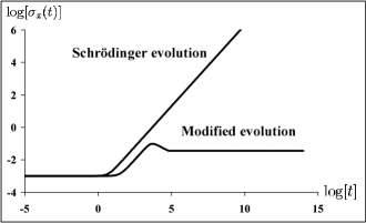
Figure 1: The picture shows the time evolution ($t$ measured in seconds) of the spread in position $\sigma_{q}(t)$ (measured in meters) of a Gaussian wavefunction, as given by the Schrödinger equation and by the stochastic equation. The simulation has been made for a nucleon ($m=m_{0}$). The initial spread has been taken equal to $10^{-3}$ m.

as we see, at the beginning the two evolutions almost coincide; as time increases, while in the standard quantum case the spread goes to infinity, the spread according to our stochastic equation reaches the asymptotic value:

$$\sigma_{q}(\infty)\;=\;\sqrt{\frac{\hbar}{m\omega}}\;\simeq\;\left(10^{-15}\sqrt{\frac{\makebox{Kg}}{m}}\,\right)\,\makebox{m},$$ (26)

which of course depends on the mass $m$ of the particle. This behavior can be understood as follows: the reduction terms (which tend to localize the wavefunction) and the standard quantum Hamiltonian (which tends to spread out the wavefunction) compete against each other until an equilibrium — the stationary solution — is reached, which depends on the values of the parameters of the model.

Also the spread in momentum changes in time, reaching the asymptotic value:

$$\sigma_{p}(\infty)\;=\;\sqrt{\frac{\hbar m\omega}{2}}\;\simeq\;\left(10^{-19}\sqrt{\frac{m}{\makebox{Kg}}}\,\right)\,\frac{\makebox{Kg m}}{\makebox{sec}}$$ (27)

It is interesting to compare the two asymptotic values for the spread in position and momentum; one has:

$$\sigma_{q}(\infty)\,\sigma_{p}(\infty)\;=\;\frac{\hbar}{\sqrt{2}}$$ (28)

which corresponds to almost the minimum allowed by Heisenberg’s uncertainty relations grw1 ; hal : the collapse model, then, induces almost the best possible localization of the wavefunction — both in position and momentum. In accordance with di1 , any Gaussian wavefunction having these asymptotic values for $\sigma_{q}$ and $\sigma_{p}$ will be called a “stationary solution” of Eq. (1).

Note the interesting fact that the evolution of the spread in position and momentum is deterministic and depends on the noise only indirectly, through the constant $\lambda$.

III.3 The mean in position and momentum

The quantities $\langle q\rangle_{t}=\overline{x}_{t}$ and $\langle p\rangle_{t}=\hbar\overline{k}_{t}$, corresponding to the peak of the Gaussian wavefunction in the position and momentum spaces, respectively, satisfy the following stochastic differential equations:

$$d\langle q\rangle_{t} = \frac{1}{m}\,\langle p\rangle_{t}dt\;+\;\sqrt{\lambda}\,\frac{1}{2a_{t}^{\makebox{\tiny R}}}\,dW_{t},$$ (29)

$$d\langle p\rangle_{t} = -\sqrt{\lambda}\hbar\,\frac{a_{t}^{\makebox{\tiny I}}}{a_{t}^{\makebox{\tiny R}}}\,dW_{t}.$$ (30)

Their average values obey the classical equations for a free particle of mass $m$:

$$m\,\frac{d}{dt}\,{\mathbb{E}}\left[\langle q\rangle_{t}\right] = {\mathbb{E}}\left[\langle p\rangle_{t}\right],$$ (31)

$${\mathbb{E}}\left[\langle p\rangle_{t}\right] = \langle p\rangle_{0},$$ (32)

while the coefficients of covariance matrix

$$C(t) = {\mathbb{E}}\left[\left[\begin{array}[]{c}\langle q\rangle_{t}-{\mathbb{E}}[\langle q\rangle_{t}]\\ \langle p\rangle_{t}-{\mathbb{E}}[\langle p\rangle_{t}]\end{array}\right]\cdot\left[\begin{array}[]{c}\langle q\rangle_{t}-{\mathbb{E}}[\langle q\rangle_{t}]\\ \langle p\rangle_{t}-{\mathbb{E}}[\langle p\rangle_{t}]\end{array}\right]^{\top}\right]$$ (40)

$$\equiv\left[\begin{array}[]{cc}C_{q^{2}}(t)&C_{qp}(t)\\ C_{pq}(t)&C_{p^{2}}(t)\end{array}\right]$$

evolve as follows:

$$\frac{d}{dt}\,C_{q^{2}}(t) = \frac{2}{m}\,C_{qp}(t)+\frac{\lambda}{4}\frac{1}{(a_{t}^{\makebox{\tiny R}})^{2}},$$ (41)

$$\frac{d}{dt}\,C_{qp}(t) = \frac{1}{m}\,C_{p^{2}}(t)-\frac{\lambda\hbar}{2}\frac{a_{t}^{\makebox{\tiny I}}}{(a_{t}^{\makebox{\tiny R}})^{2}},$$ (42)

$$\frac{d}{dt}\,C_{p^{2}}(t) = \lambda\hbar^{2}\left(\frac{a_{t}^{\makebox{\tiny I}}}{a_{t}^{\makebox{\tiny R}}}\right)^{2}.$$ (43)

Particularly interesting is the third equation, which implies that the wavefunction picks larger and larger components in momentum, as time increases; as a consequence, the energy of the system increases in time, as it can be seen by writing down the stochastic differential for $\langle H\rangle_{t}\equiv\langle p^{2}\rangle_{t}/2m$:

$$d\langle H\rangle_{t}\;=\;\frac{\lambda\hbar^{2}}{2m}\,dt\;-\;\sqrt{\lambda}\,\frac{\hbar}{m}\,\frac{a_{t}^{\makebox{\tiny I}}}{a_{t}^{\makebox{\tiny R}}}\,\langle p\rangle_{t}\,dW_{t},$$ (44)

from which it follows that:

$$\frac{d}{dt}\,{\mathbb{E}}[\langle H\rangle_{t}]\;=\;\frac{\lambda\hbar^{2}}{2m}\;=\;\frac{\lambda_{0}\hbar^{2}}{2m_{0}}\;\simeq\;10^{-43}\;\makebox{J/sec}.$$ (45)

This energy non–conservation is a typical feature of space–collapse models, but with our choice for the parameter $\lambda$, the increase is so weak that it cannot be detected with present–day technology (see ref. grw1 ).

IV Double Gaussian solution

We now study the time evolution of the superposition of two Gaussian wavefunctions; such an analysis is interesting since it allows to understand in a quite simple and clear way how the reduction mechanism works, i.e. how the superposition of two different position states is reduced into one of them. To this purpose, let us consider the following wavefunction:

$$\phi_{t}^{\makebox{\tiny D}}(x) = \phi_{1t}(x)\,+\,\phi_{2t}(x)\;=\;$$ (46)

$$= \makebox{exp}\left[-a_{1t}(x-\overline{x}_{1t})^{2}+i\overline{k}_{1t}x+\gamma_{1t}\right]$$

$$+ \makebox{exp}\left[-a_{2t}(x-\overline{x}_{2t})^{2}+i\overline{k}_{2t}x+\gamma_{2t}\right];$$

we follow the strategy outlined in Sec. II, by first finding the solution of the linear equation.

Because of linearity, $\phi_{t}^{\makebox{\tiny D}}(x)$ is automatically a solution of Eq. (4), provided that its parameters satisfy Eqs. (9) to (13). The difficult part of the analysis is related to the change of measure: the reason is that in the double–Gaussian case the quantum average $\langle q\rangle_{t}$ is not simply equal to $\overline{x}_{1t}$ or $\overline{x}_{2t}$, as it is for a single–Gaussian wavefunction, but is a nontrivial function of all the parameters defining $\phi_{t}^{\makebox{\tiny D}}(x)$; in spite of this difficulty, the most interesting properties of the dynamical evolution of $\phi_{t}^{\makebox{\tiny D}}(x)$ can be analyzed in a rigorous way.

We first observe that the two equations for $a_{1t}$ and $a_{2t}$ are deterministic and thus insensitive of the change of measure; accordingly, the spread (both in position and in momentum) of the two Gaussian functions defining $\phi_{t}^{\makebox{\tiny D}}(x)$ evolve independently of each other, and maintain all the properties discussed in the previous section. For simplicity, we assume that $a_{1t}=a_{2t}$ at $t=0$ so that these two parameters will remain equal at any subsequent time.

IV.1 The asymptotic behavior

Let us consider the differences $X_{t}=\overline{x}_{2t}-\overline{x}_{1t}$ and $K_{t}=\overline{k}_{2t}-\overline{k}_{1t}$ between the peaks of the two Gaussian functions in the position and in the momentum spaces; they satisfy the following set of equations:

$$d\left[\begin{array}[]{c}X_{t}\\ K_{t}\end{array}\right]\;=\;\left[\begin{array}[]{cc}-A_{1}(t)&\hbar/m\\ -A_{2}(t)&0\end{array}\right]\cdot\left[\begin{array}[]{c}X_{t}\\ K_{t}\end{array}\right]\,dt,$$ (47)

with:

$$A_{1}(t) = \;\omega\,\frac{\cosh(\omega t+\varphi_{1})+\cos(\omega t+\varphi_{2})}{\sinh(\omega t+\varphi_{1})+\sin(\omega t+\varphi_{2})},$$ (48)

$$A_{2}(t) = 2\lambda\,\frac{\sinh(\omega t+\varphi_{1})-\sin(\omega t+\varphi_{2})}{\sinh(\omega t+\varphi_{1})+\sin(\omega t+\varphi_{2})}.$$ (49)

We see — this is the reason why we have taken into account the differences $X_{t}$ and $K_{t}$ — that the above system of equations is deterministic, so it does not depend on the change of measure.

The coefficients of the $2\times 2$ matrix $A(t)$ defining the linear system (47) are analytic in the variable $t$, and the Liapunov’s type numbers ltn of the system are the same as those of the linear system obtained by replacing $A(t)$ with $A(\infty)$, where:

$$A(\infty)\;\equiv\;\lim_{t\rightarrow+\infty}\,A(t)\;=\;\left[\begin{array}[]{cc}-\omega&\hbar/m\\ -2\lambda&0\end{array}\right].$$ (50)

The eigenvalues of the matrix $A(\infty)$ are:

$$\mu_{1,2}\;=\;-\frac{1}{2}\,\left(1\pm i\right)\,\omega,$$ (51)

from which it follows that the linear system (47) has only one Lyapunov’s type number: $-\omega/2$. This implies that, for any non trivial (vector) solution ${\bf Z}(t)$ of (47), one has:

$$\lim_{t\rightarrow+\infty}\,\frac{\ln|{\bf Z}(t)|}{t}\;=\;-\frac{\omega}{2}\quad\Rightarrow\quad\lim_{t\rightarrow+\infty}\,{\bf Z}(t)\;=\;{\bf 0}.$$ (52)

We arrive at the following result: asymptotically, the difference $\overline{x}_{2t}-\overline{x}_{1t}$ between the peaks of the two Gaussian wavefunctions in the position space goes to zero; also the difference $\overline{k}_{2t}-\overline{k}_{1t}$ between the peaks of the two Gaussian wavefunctions in the momentum space vanishes. In other words, the two Gaussian wavefunctions converge toward each other, and asymptotically they become one single–Gaussian wavefunction which, from the analysis of the previous subsection, is a “stationary” solution of the stochastic equation (1).

Anyway, this behavior in general cannot be responsible for the collapse of a macroscopic superposition; as a matter of fact, let us consider the following situation which, for later convenience, we call “situation ${\mathcal{A}}$”:

i) The wavefunction is in a superposition of the form (46) and, at time $t=0$ (consequently, also for any later $t$), $a_{1t}$ and $a_{2t}$ are equal to their asymptotic value;

ii) The distance $K_{t}\equiv\overline{k}_{2t}-\overline{k}_{1t}$ is zero at time $t=0$.

Under these assumptions, the linear system (47) can be easily solved and one gets:

$$X_{t}\;=\;X_{0}\,e^{\displaystyle-\omega t/2}\,\left[\cos\frac{\omega t}{2}-\sin\frac{\omega t}{2}\right].$$ (53)

We see that the time evolution of $X_{t}$ is independent of the mass of the particle: this result implies that, when the spread of the two Gaussian wavefunctions is equal to its asymptotic value, their distance decreases with a rate $\omega/2\sim 10^{-5}$ sec^-1, which is too slow to justify a possible collapse, in particular at the macro–level.

IV.2 The collapse

Now we show that the collapse of the wavefunction occurs because, during the evolution, one of the two Gaussian wavefunctions is suppressed with respect to the other one; the quantity which measure this damping is the difference $\Gamma_{t}^{\makebox{\tiny R}}=\gamma_{2t}^{\makebox{\tiny R}}-\gamma_{1t}^{\makebox{\tiny R}}$, which satisfies the stochastic differential equation:

$$d\Gamma_{t}^{\makebox{\tiny R}}=-\lambda X_{t}\left[\overline{x}_{1t}+\overline{x}_{2t}-2\langle q\rangle_{t}\right]dt+\sqrt{\lambda}X_{t}dW_{t};$$ (54)

if $\Gamma_{t}^{\makebox{\tiny R}}\rightarrow+\infty$, then $\phi_{1}$ is suppressed with respect to $\phi_{2}$ and the superposition practically reduces to $\phi_{2}$; the opposite happens if $\Gamma_{t}^{\makebox{\tiny R}}\rightarrow-\infty$.

To be more precise, we introduce a positive constant $b$ which we assume to be conveniently large (let us say, $b=10$) and we say that the superposition is suppressed when $|\Gamma^{\makebox{\tiny R}}|\geq b$; moreover, we say that:

$$\phi^{\makebox{\tiny D}} \phi_{1} \Gamma^{\makebox{\tiny R}}\leq-b,$$ is reduced to when:

$$\phi^{\makebox{\tiny D}} \phi_{2} \Gamma^{\makebox{\tiny R}}\geq+b.$$ is reduced to when:

We now study the time evolution of $\Gamma_{t}^{\makebox{\tiny R}}$.

By writing $\langle q\rangle_{t}$ in terms of the coefficients defining $\phi_{t}^{\makebox{\tiny D}}(x)$:

$$\langle q\rangle_{t}\;=\;\sqrt{\frac{\pi}{2a_{t}^{\makebox{\tiny R}}}}\,\left[\overline{x}_{1t}e^{2\gamma_{1t}^{\makebox{\tiny R}}}+\overline{x}_{2t}e^{2\gamma_{2t}^{\makebox{\tiny R}}}+\delta_{t}e^{\gamma_{1t}^{\makebox{\tiny R}}+\gamma_{2t}^{\makebox{\tiny R}}}\right]$$ (55)

it is not difficult to prove that Eq. (54) becomes:

$$d\Gamma_{t}^{\makebox{\tiny R}}=\lambda X_{t}^{2}\,\tanh\Gamma_{t}^{\makebox{\tiny R}}\,dt\,+\,g_{t}(\Gamma_{t}^{\makebox{\tiny R}})\,dt\,+\,\sqrt{\lambda}X_{t}\,dW_{t},$$ (56)

where we have defined the following quantities:

$$\delta_{t} = h_{t}\left[(\overline{x}_{1t}+\overline{x}_{2t})\cos\theta_{t}+Y_{t}\sin\theta_{t}\right],$$ (57)

$$g_{t}(\Gamma_{t}^{\makebox{\tiny R}}) = 2\lambda X_{t}h_{t}e^{\Gamma_{t}^{\makebox{\tiny R}}}\cdot$$

$$\frac{Y_{t}\sin\theta_{t}\left[1+e^{2\Gamma_{t}^{\makebox{\tiny R}}}\right]+X_{t}\cos\theta_{t}\left[1-e^{2\Gamma_{t}^{\makebox{\tiny R}}}\right]}{\left[1+e^{2\Gamma_{t}^{\makebox{\tiny R}}}+2h_{t}\cos\theta_{t}e^{\Gamma_{t}^{\makebox{\tiny R}}}\right]\left[1+e^{2\Gamma_{t}^{\makebox{\tiny R}}}\right]}$$

and:

$$h_{t} = \exp\left[-\frac{a_{t}^{\makebox{\tiny R}}}{2}\left(X^{2}_{t}+Y_{t}^{2}\right)\right],$$ (59)

$$Y_{t} = -\frac{2a_{t}^{\makebox{\tiny I}}X_{t}+K_{t}}{2a_{t}^{\makebox{\tiny R}}},$$ (60)

$$\theta_{t} = \frac{1}{2}\,\left(\overline{x}_{1t}+\overline{x}_{2t}\right)K_{t}+\Gamma_{t}^{\makebox{\tiny I}},\qquad\Gamma_{t}^{\makebox{\tiny I}}=\gamma_{2t}^{\makebox{\tiny I}}-\gamma_{1t}^{\makebox{\tiny I}},\qquad$$ (61)

with $a_{t}^{\makebox{\tiny R}}\equiv a_{1t}^{\makebox{\tiny R}}=a_{2t}^{\makebox{\tiny R}}$.

Eq. (56) cannot be solved exactly, due to the presence of the term $g_{t}(\Gamma_{t}^{\makebox{\tiny R}})$ which is a non–simple function of $\Gamma_{t}^{\makebox{\tiny R}}$; to circumvent this problem, we proceed as follows. We study the following stochastic differential equation:

$$d{\tilde{\Gamma}}_{t}^{\makebox{\tiny R}}=\lambda X_{t}^{2}\,\tanh{\tilde{\Gamma}}_{t}^{\makebox{\tiny R}}\,dt\,+\,\sqrt{\lambda}X_{t}\,dW_{t},$$ (62)

which corresponds to Eq. (56) without the term $g_{t}(\Gamma_{t}^{\makebox{\tiny R}})$, and at the end of the subsection we estimate the error made by ignoring such a term.

In studying Eq. (62), it is convenient to introduce the following time–change:

$$t\;\longrightarrow\;s_{t}\;=\;\lambda\int_{0}^{t}X_{u}^{2}\,du.$$ (63)

$X_{t}^{2}$ is a continuous, differentiable and non–negative function, which we can assume not to be identically zero in any sub–interval of ${\mathbb{R}}^{+}$; as a consequence, $s_{t}$ is a monotone increasing — thus invertible — function of $t$ and Eq. (63) defines a good time change.

Under this time substitution, Eq. (62) becomes:

$$d{\tilde{\Gamma}}_{s}^{\makebox{\tiny R}}=\tanh{\tilde{\Gamma}}_{s}^{\makebox{\tiny R}}\,ds\,+\,d{\tilde{W}}_{s},$$ (64)

where

$${\tilde{W}}_{s}\;=\;\sqrt{\lambda}\,\int_{0}^{s}X_{t}\,dW_{t}$$ (65)

is a Wiener process with respect to the filtered space $(\Omega,{\mathcal{F}},\{{\mathcal{F}}_{s}:s\geq 0\},{\mathbb{P}})$. Note that, since according to Eq. (52), $X_{t}$ in general decays exponentially in time, $s_{\infty}<\infty$, and Eq. (64) is physically meaningful only within the interval $[0,s_{\infty})$.

Eq. (64) can be analyzed in great detail gsb ; in particular, the following properties can be proven to hold:

1. Let us define the collapse time $S_{b}\equiv\inf\{s:|{\tilde{\Gamma}}_{s}^{\makebox{\tiny R}}|\,\geq\,b\}$: this time is finite with probability 1 and its average value is equal to:

$${\mathbb{E}}[S_{b}]\;=\;b\tanh b\,-\,b_{0}\tanh b_{0}.$$ (66)

If $b_{0}\ll b$ (which occurs when both terms of the superposition give a non–vanishing contribution), and since we have assumed $b\simeq 10$, then ${\mathbb{E}}[S_{b}]\simeq b$.

2. The variance ${\mathbb{V}}[S_{b}]\equiv{\mathbb{E}}[S_{b}^{2}]-{\mathbb{E}}^{2}[S_{b}]$ is given by:

$${\mathbb{V}}[S_{b}]\;=\;F(b)\,-\,F(b_{0}),$$ (67)

with:

$$F(x)=x^{2}\tanh^{2}x+x\tanh x-x^{2}.$$ (68)

Note that since $F(x)$ is an even, positive function, increasing for positive values of $x$, it follows that ${\mathbb{V}}[S_{b}]>0$ whenever $|b_{0}|<b$, as it assumed to be.

3. The collapse probability $P_{\phi_{2}}$ that $\phi^{\makebox{\tiny D}}$ is reduced to $\phi_{2}$, i.e. that ${\tilde{\Gamma}}_{s}^{\makebox{\tiny R}}$ hits point $b$ before point $-b$ is given by:

$$P_{\phi_{2}}\;=\;\frac{1}{2}\,\frac{\tanh b+\tanh b_{0}}{\tanh b};$$ (69)

according to our choice for $b$, $\tanh b\simeq 1$, and consequently

$$P_{\phi_{2}} \simeq \frac{1}{2}\,[1+\tanh b_{0}]\;=\;\frac{e^{2\gamma_{20}^{\makebox{\tiny R}}}}{e^{2\gamma_{10}^{\makebox{\tiny R}}}+e^{2\gamma_{20}^{\makebox{\tiny R}}}}\;=$$ (70)

$$= \frac{\|\phi_{20}\|^{2}}{\|\phi_{10}\|^{2}+\|\phi_{20}\|^{2}},$$

which (neglecting the overlapping between the two Gaussian wavefunctions) corresponds to the standard quantum prescription for the probability that $\phi^{\makebox{\tiny D}}$ collapses to $\phi_{2}$.

4. The delocalization probability, i.e. the probability $P_{\phi_{2}}^{\makebox{\tiny Del}}$ that ${\tilde{\Gamma}}_{t}^{\makebox{\tiny R}}$ goes below $b-\eta$ before time $s_{\infty}$, after having reached $b$ ($\eta$ is a positive quantity smaller than $b$), is:

$$P_{\phi_{2}}^{\makebox{\tiny Del}} \leq 1\;-\;P\{\inf{\tilde{\Gamma}}_{s}^{\makebox{\tiny R}}>b-\eta\}\;=\;$$ (71)

$$= 1\;-\;(1+\tanh b)\,\frac{\tanh\eta}{1+\tanh\eta}.$$

In the above definition, we have required a delocalization to occur before time $s_{\infty}$ because — since $s_{\infty}$ corresponds to $t=\infty$ — a delocalization at a time $\geq s_{\infty}$ does not correspond to a real physical delocalization.

If, for example, we take $\eta=3$, we have that $P_{\phi_{2}}^{\makebox{\tiny Del}}\lesssim 0.002$.

This concludes our analysis of the statistical behavior of ${\tilde{\Gamma}}_{s}^{\makebox{\tiny R}}$. We end this section by discussing how one can estimate the error made in neglecting the term $g_{t}(\Gamma_{t}^{\makebox{\tiny R}})$ in Eq. (56), i.e. in studying ${\tilde{\Gamma}}_{s}^{\makebox{\tiny R}}$ in place of $\Gamma_{s}^{\makebox{\tiny R}}$. In Appendix A the following estimate for $g_{t}(\Gamma_{t}^{\makebox{\tiny R}})$ is given:

$$\left|g_{t}(\Gamma_{t}^{\makebox{\tiny R}})\right| \leq \lambda\frac{(|X_{t}|+|Y_{t}|)^{2}}{e^{a_{t}^{\makebox{\tiny R}}(|X_{t}|+|Y_{t}|)^{2}/4}-1}$$ (72)

$$\leq \frac{\lambda X_{t}^{2}}{e^{a_{m}^{\makebox{\tiny R}}\,X_{m}^{2}/4}-1},$$ (73)

where $a_{m}^{\makebox{\tiny R}}$ and $X_{m}$ are the minimum values $a_{t}^{\makebox{\tiny R}}$ and $X_{t}$ take during the time interval one is considering. For example, if we take a 1–g object and we assume that $a_{m}^{\makebox{\tiny R}}=a_{\infty}^{\makebox{\tiny R}}$ and $X_{m}=1$ cm, then we have:

$$c\;\equiv\;\frac{1}{e^{a_{m}^{\makebox{\tiny R}}\,X_{m}^{2}/4}-1}\;\simeq\;e^{-10^{21}},$$ (74)

which is very close to zero.

By using inequality (73) and lemma 4, pag. 120 of gsb , one can easily show that $\Gamma_{s}^{\makebox{\tiny R}-}\leq\Gamma_{s}^{\makebox{\tiny R}}\leq\Gamma_{s}^{\makebox{\tiny R}+}$, where $\Gamma_{s}^{\makebox{\tiny R}\pm}$ are solutions of the following two stochastic differential equations:

$$d\Gamma_{s}^{\makebox{\tiny R}\pm}\;=\;\left[\tanh{\Gamma}_{s}^{\makebox{\tiny R}\pm}\pm c\right]ds\,+\,d{\tilde{W}}_{s},$$ (75)

with an obvious meaning of the signs (as before, we have moved from the variable $t$ to the variable $s$).

Eqs. (75) can be analyzed along the same lines followed in studying Eq. (64), getting basically the same results, due to the very small value $c$ takes in most relevant physical situations. This kind of analysis will be done in detail in a future paper: there, we will study the most important case where a macroscopic superposition can be created, i.e. a measurement–like situation in which a macroscopic object acting like a measuring apparatus interacts with a microscopic system being initially in a superposition of two eigenstates of the operator which is measured; we will show that, throughout the interaction, the wavefunction of the apparatus is — with extremely high probability — always localized in space, and that the measurement has a definite outcome with the correct quantum probabilities.

V General solution: the asymptotic behavior

In this section we analyze the asymptotic behavior of the general solution of Eq. (1), showing that — as time increases — any wavefunction collapses towards a stationary Gaussian solution.

V.1 The collapse

We have seen in the previous sections that both the single–Gaussian and double–Gaussian solutions asymptotically converge towards a stationary solution having the form:

$$\psi_{t}(x)\;=\;\sqrt[4]{\frac{2a^{\makebox{\tiny R}}_{\infty}}{\pi}}\,\exp\left[-a_{\infty}(x-\overline{x}_{t})^{2}+i\overline{k}_{t}x\right],$$ (76)

with:

$$a_{\infty}\;=\;\lim_{t\rightarrow+\infty}a_{t}\;=\;\frac{\lambda}{\omega}(1-i);$$ (77)

it becomes then natural to ask whether such a kind of wavefunction is the asymptotic limit of any initial wavefunction. The answer is positive hal as we shall now see by following the same strategy used in refs. jp2 ; ad2 ; hal to prove convergence of solutions.

Since a wavefunction of the form (76) is an eigenstate of the operator:

$$A\;=\;q\,+\,\frac{i-1}{m\omega}\,p,$$ (78)

the proof consists in showing that the variance:

$$\Delta A_{t}\;\equiv\;\langle\psi_{t}|[A^{\dagger}-\langle A^{\dagger}\rangle][A-\langle A\rangle]|\psi_{t}\rangle$$ (79)

converges to 0 for $t\rightarrow+\infty$. The following expression for $\Delta A_{t}$ holds:

$$\Delta A_{t}\;=\;\Delta q_{t}+\frac{2}{m^{2}\omega^{2}}\Delta p_{t}-\frac{2}{m\omega}\Sigma(q,p)-\frac{\hbar}{m\omega},$$ (80)

with:

$$\Sigma(q,p) = \frac{1}{2}\left[\langle\psi_{t}|[q-\langle q\rangle][p-\langle p\rangle]|\psi_{t}\rangle+\right.$$ (81)

$$\;\;\;\;\left.\langle\psi_{t}|[p-\langle p\rangle][q-\langle q\rangle]|\psi_{t}\rangle\right]$$

After a rather long calculation, one finds that:

$$\frac{d}{dt}\,{\mathbb{E}}\left[\Delta A_{t}\right] = -{\mathbb{E}}\left[\omega\,\Delta A_{t}+2\lambda\,\left(\Delta q_{t}-\sigma_{q}^{2}(\infty)\right)^{2}\right.$$

$$\left.+2\lambda\,\left(\Delta q_{t}-\frac{2}{m\omega}\,\Sigma(q,p)\right)^{2}\right]\;\leq\;0.$$

Since, by definition, ${\mathbb{E}}\left[\Delta A_{t}\right]$ is a non–negative quantity, Eq. (V.1) is consistent if and only if the right–hand–side asymptotically vanishes. This, in particular, implies that

$$\Delta A_{t}\;\xrightarrow[t\,\rightarrow\,+\infty]{}\;0,$$ (83)

except for a subset of $\Omega$ of measure zero.

V.2 The collapse probability

We now analyze the probability that the wavefunction, as a result of the collapse process, lies within a given region of space. To this purpose, let us consider the following probability measure, defined on the Borel sigma–algebra ${\mathcal{B}}({\mathbb{R}})$:

$$\mu_{t}(\Delta)\;\equiv\;{\mathbb{E}}_{{\mathbb{P}}}\left[\|P_{\Delta}\psi_{t}\|^{2}\right],$$ (84)

where $P_{\Delta}$ is the projection operator associated to the Borel subset $\Delta$ of ${\mathbb{R}}$. Such a measure is identified by the density $p_{t}(x)\equiv{\mathbb{E}}_{{\mathbb{P}}}[|\psi_{t}(x)|^{2}]$:

$$\mu_{t}(\Delta)\;=\;\int_{\Delta}p_{t}(x)\,dx,$$ (85)

and it can be easily shown that the density $p_{t}(x)$ corresponds to the diagonal element $\langle x|\rho_{t}|x\rangle$ of the statistical operator$\rho_{t}\equiv{\mathbb{E}}_{{\mathbb{P}}}\left[|\psi_{t}\rangle\langle\psi_{t}|\right]$, which satisfies the Lindblad–type equation:

$$\frac{d}{dt}\,\rho_{t}\;=\;-\frac{i}{2m\hbar}\,\left[p^{2},\rho_{t}\right]-\frac{\lambda}{2}\left[q,\left[q,\rho_{t}\right]\right].$$ (86)

The solution of the above equation, expressed in terms of the solution $\langle q_{1}|\rho_{S}(t)|q_{2}\rangle$ of the pure Schrödinger equation ($\lambda=0$), is:

$$\langle q_{1}|\rho(t)|q_{2}\rangle\;=\;\frac{1}{2\pi\hbar}\int_{-\infty}^{+\infty}dk\int_{-\infty}^{+\infty}dy\,e^{-(i/\hbar)ky}F[k,q_{1}-q_{2},t]\langle q_{1}+y|\rho_{S}(t)|q_{2}+y\rangle,$$ (87)

with:

$$F[k,x,t]\;=\;\exp\left[-\frac{\lambda}{2}\,t\,\left(x^{2}-\frac{k}{m}\,xt+\frac{k^{2}}{3m^{2}}t^{2}\right)\right].$$ (88)

The Hermitian symmetry of $\langle q_{1}|\rho(t)|q_{2}\rangle$ follows from the fact that $F[k,x,t]=F[-k,-x,t]$; for $\lambda=0$ we have $F[k,x,t]=1$ so that $\langle q_{1}|\rho(t)|q_{2}\rangle=\langle q_{1}|\rho_{S}(t)|q_{2}\rangle$ as it must be.

From Eq. (87) it follows that:

$$p_{t}(x)=\frac{1}{2\pi\hbar}\int_{-\infty}^{+\infty}dk\int_{-\infty}^{+\infty}dy\,e^{-(i/\hbar)ky}F[k,0,t]p_{t}^{S}(x+y)$$ (89)

where $p_{t}^{S}(x)=\langle x|\rho_{S}(t)|x\rangle$ is the standard quantum probability density of finding the particle located $x$ in a position measurement. One can easily perform the integration over the $k$ variable and he gets:

$$p_{t}(x)\;=\;\sqrt{\frac{\alpha_{t}}{\pi}}\int_{-\infty}^{+\infty}dy\,e^{-\alpha_{t}y^{2}}p_{t}^{S}(x+y),$$ (90)

with:

$$\alpha_{t}\;=\;\frac{3m_{0}}{2\hbar^{2}\lambda_{0}}\,\frac{m}{t^{3}}\;\simeq\;10^{43}\left(\frac{m}{\makebox{kg}}\right)\left(\frac{\makebox{sec}}{t}\right)^{3}.$$ (91)

For a macroscopic object (let us say $m\geq 1$ g) and for very long times (e.g. $t\in[0,10^{8}$ sec $\simeq$ 3 years], a time interval which of course is much longer than the time during which an object can be kept isolated so that the free particle approximation holds true) $\alpha_{t}$ is a very large number, so large that the exponential function in Eq. (90) is significantly more narrow than $p_{t}^{S}(x)$, for most typical wavefunctions (in Sec. VII.1 we will see that the asymptotic spread of the wavefunction of a 1–g object is about $10^{-13}$ m). Accordingly, this exponential function acts like a Dirac–delta and one has: $p_{t}(x)\simeq p^{S}_{t}(x)$, with very high accuracy. This in turn implies that:

$$\mu_{t}(\Delta)\;\simeq\;\|P_{\Delta}\psi^{\makebox{\tiny Sch}}_{t}\|^{2}:$$ (92)

in other words, the probability measure $\mu_{t}(\Delta)$ is very close to the quantum probability of finding the particle lying in $\Delta$ in a position measurement.

We still have to discuss the physical meaning of the probability measure $\mu_{t}(\Delta)$ defined by Eq. (84); such a discussion is relevant only at the macroscopic level, since we need only macro–objects to be well localized in space (and with the correct quantum probabilities).

As already anticipated the spread of a wavefunction of a macro–object having the mass of e.g. 1 g reaches in a very short time a value which is close to the asymptotic spread $\sigma_{q}(\infty)\simeq 10^{-13}$ m; then, if we take for $\Delta$ an interval $[a,b]$ whose length is much greater than $\sigma_{q}(\infty)$ — for example, we can take $b-a=10^{-7}$ m, which is sufficiently small for all practical purposes — only those wavefunctions whose mean lies around $\Delta$ give a non vanishing contribution to $\mu_{t}(\Delta)$. As a consequence, with the above choices for $\Delta$ (and, of course, waiting a time sufficiently long in order for the reduction to have occurred), the measure $\mu_{t}(\Delta)$ represents a good probability measure that the wavefunction collapses within $\Delta$.

VI Effect of the reducing terms on the microscopic dynamics

In the previous sections we have studied some analytical properties of the solutions of the stochastic differential equation (1); we now focus our attention on the dynamics for a microscopic particle.

The time evolution of a (free) quantum particle has three characteristic features:

1. The wavefunction is subject to a localization process, which, at the micro–level, is extremely slow, almost negligible. For example, with reference to the situation ${\mathcal{A}}$ we have defined at the end of Sec. IV.1, Eq. (53) shows that the distance $X_{t}$ between the centers of the two Gaussian wavefunctions remains practically unaltered for about $10^{5}$ sec; under the approximation $X_{t}\simeq X_{0}$, Eqs. (63) and (66) imply that the time necessary for one of the two Gaussians to be suppressed is:

$${\mathbb{E}}\left[T_{b}\right] \simeq 10^{6}\,\left(\frac{\makebox{m}}{X_{0}}\right)^{2}\;\makebox{sec $\quad$ for an electron,}$$

$${\mathbb{E}}\left[T_{b}\right] \simeq 10^{3}\,\left(\frac{\makebox{m}}{X_{0}}\right)^{2}\;\makebox{sec $\quad$ for a nucleon,}$$

which are very long times, compared with the characteristic times of a quantum experiment.

2. The spread of the wavefunction reaches an asymptotic value which depends on the mass of the particle:

$$\sigma_{q}(\infty) \simeq 1\;\makebox{m $\quad\;\,$ for an electron,}$$

$$\sigma_{q}(\infty) \simeq 1\;\makebox{cm $\quad$ for a nucleon.}$$

3. The wavefunction undergoes a random motion both in position and momentum, under the influence of the stochastic process. These fluctuations can be quite relevant at the microscopic level; for example, for a stationary solution, one has from Eq. (41):

$$\frac{d}{dt}\,{\mathbb{V}}\left[\langle q\rangle_{t}\right] \geq 1\quad\!\makebox{m${}^{2}$/sec $\qquad$ for an electron,}$$

$$\frac{d}{dt}\,{\mathbb{V}}\left[\langle q\rangle_{t}\right] \geq 10^{-3}\;\makebox{m${}^{2}$/sec $\quad$ for a nucleon.}$$

This is the physical picture of a microscopic particle as it emerges from the collapse model. In order for the model to be physically consistent, it must reproduce at the microscopic level the predictions of standard quantum mechanics, an issue which we are now going to discuss.

Within the collapse model, measurable quantities are given mis by averages of the form ${\mathbb{E}}_{{\mathbb{P}}}[\langle O\rangle_{t}]$, where $O$ is (in principle) any self–adjoint operator. It is not difficult to prove that:

$${\mathbb{E}}_{{\mathbb{P}}}\left[\langle O\rangle_{t}\right]\;=\;\makebox{Tr}\left[O\rho_{t}\right],$$ (93)

where the statistical operator $\rho_{t}\equiv{\mathbb{E}}_{{\mathbb{P}}}\left[|\psi_{t}\rangle\langle\psi_{t}|\right]$ satisfies the Lindblad–type Eq. (86). This is a typical master equation used in decoherence theory to describe the interaction between a quantum particle and the surrounding environment dec1 ; consequently, as far as experimental results are concerned, the predictions of our model are similar to those of decoherence models. It becomes then natural to compare the strength of the collapse mechanism (measured by the parameter $\lambda$) with that of decoherence.

Such a comparison is given in Table 1, when the system under study is a very small particle like an electron, or an almost macroscopic object like a dust particle.

Cause of decoherence	$10^{-3}$ cm	$10^{-6}$ cm
	dust particle	large molecule
Air molecules	$10^{36}$	$10^{30}$
Laboratory vacuum	$10^{23}$	$10^{17}$
Sunlight on earth	$10^{21}$	$10^{13}$
300K photons	$10^{19}$	$10^{6}$
Cosmic background rad.	$10^{6}$	$10^{-12}$
COLLAPSE	$10^{7}$	$10^{-2}$

Table 1: $\lambda$ in cm^-2sec^-1 for decoherence arising from different kinds of scattering processes (taken from Joos and Zeh dec1 ). In the last line: $\lambda$ for the collapse model given by Eq. (1).

We see that, for most sources of decoherence, the experimentally testable effects of the collapse mechanism are weaker than those produced by the interaction with the surrounding environment. This implies that, in order to test such effects, one has to isolate a quantum system — for a sufficiently long time — from almost all conceivable sources of decoherence, which is quite difficult: the experimentally testable differences between our collapse model and standard quantum mechanics are so small that they cannot be detected unless very sophisticated experiments are performed pref ; exp .

VII Multi–particle systems: effect of the reducing terms on the macroscopic dynamics

The generalization of Eq. (1) to a system of $N$ interacting and distinguishable particles is straightforward:

$$d\,\psi_{t}(\{x\}) = \left[-\frac{i}{\hbar}\,H_{\makebox{\tiny T}}\,dt+\sum_{n=1}^{N}\sqrt{\lambda_{n}}\,(q_{n}-\langle q_{n}\rangle_{t})\,dW_{t}^{n}\right.$$ (94)

$$\left.-\frac{1}{2}\,\sum_{n=1}^{N}\lambda_{n}(q_{n}-\langle q_{n}\rangle_{t})^{2}dt\right]\psi_{t}(\{x\}),$$

where $H_{\makebox{\tiny T}}$ is the standard quantum Hamiltonian of the composite system, the operators $q_{n}$ ($n=1,\ldots N$) are the position operators of the particles of the system, and $W_{t}^{n}$ ($n=1,\ldots N$) are $N$ independent standard Wiener processes; the symbol $\{x\}$ denotes the $N$ spatial coordinates $x_{1},\ldots x_{N}$.

For the purposes of our analysis, it is convenient to switch to the center–of–mass ($R$) and relative ($\tilde{x}_{1},\tilde{x}_{2},\ldots\tilde{x}_{N}$) coordinates:

$$\left\{\begin{array}[]{lcl}R&=&\displaystyle\frac{1}{M}\,\sum_{n=1}^{N}m_{n}\,x_{n}\qquad M\;=\;\sum_{n=1}^{N}m_{n},\\ &&\\ x_{n}&=&R+\tilde{x}_{n};\end{array}\right.$$ (95)

let $Q$ be the position operator for the center of mass and $\tilde{q}_{n}$ ($n=1\ldots N$) the position operators associated to the relative coordinates.

It is not difficult to show that — under the assumption $H_{\makebox{\tiny T}}=H_{\makebox{\tiny CM}}+H_{\makebox{\tiny rel}}$ — the dynamics for the center of mass and that for the relative motion decouple; in other words, $\psi_{t}(\{x\})=\psi_{t}^{\makebox{\tiny CM}}(R)\otimes\psi_{t}^{\makebox{\tiny rel}}(\{\tilde{x}\})$ solves Eq. (94) whenever $\psi_{t}^{\makebox{\tiny CM}}(R)$ and $\psi_{t}^{\makebox{\tiny rel}}(\{\tilde{x}\})$ satisfy the following equations:

$$d\,\psi_{t}^{\makebox{\tiny rel}}(\{\tilde{x}\}) = \left[-\frac{i}{\hbar}\,H_{\makebox{\tiny rel}}\,dt+\sum_{n=1}^{N}\sqrt{\lambda_{n}}\,({\tilde{q}}_{n}-\langle{\tilde{q}}_{n}\rangle_{t})dW_{t}^{n}\right.$$ (96)

$$\left.-\frac{1}{2}\,\sum_{n=1}^{N}\lambda_{n}({\tilde{q}}_{n}-\langle{\tilde{q}}_{n}\rangle_{t})^{2}dt\right]\psi_{t}^{\makebox{\tiny rel}}(\{x\}),$$

$$d\,\psi_{t}^{\makebox{\tiny CM}}(R) = \left[-\frac{i}{\hbar}\,H_{\makebox{\tiny CM}}\,dt+\sqrt{\lambda_{\makebox{\tiny CM}}}\,(Q-\langle Q\rangle_{t})dW_{t}\right.$$ (97)

$$\left.-\frac{\lambda_{\makebox{\tiny CM}}}{2}\,(Q-\langle Q\rangle_{t})^{2}dt\right]\psi_{t}^{\makebox{\tiny CM}}(R),$$

with:

$$\lambda_{\makebox{\tiny CM}}\;=\;\sum_{n=1}^{N}\lambda_{n}\;=\;\frac{M}{m_{0}}\,\lambda_{0}.$$ (98)

The first of the above equations describes the internal motion of the composite system, and will not be analyzed in this paper; in the remainder of the section, we will focus our attention on the second equation.

Eq. (97) shows that the reducing terms associated to the center of mass of a composite system are equal to those associated to a particle having mass equal to the total mass $M$ of the composite system; in particular, when the system is isolated — i.e., $H_{\makebox{\tiny CM}}=P^{2}/2M$, where $P$ is the total momentum — the center of mass behaves like a free particle, whose dynamics has been already analyzed in Sects. III, IV and V. In the next subsections we will see that, because of the large mass of a macro–object, the dynamics of its center of mass is radically different from that of a microscopic particle.

VII.1 The amplification mechanism

The first important feature of collapse models is what has been called the “amplification mechanism” grw1 ; grw2 : the reduction rates of the constituents of a macro–object sum up, so that the reduction rate associated to its center of mass is much greater than the reduction rates of the single constituents.

This situation is exemplified in Fig. 2, which shows the time evolution of the spread $\sigma_{q}(t)$ of a Gaussian wavefunction.

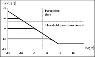
Figure 2: Time evolution of the spread $\sigma_{q}(t)$ of a Gaussian wavefunction of the center of mass of a system containing $N=10^{24}$ nucleons; different initial conditions have been considered. Time is measured in seconds, while the spread is measured in meters.

We note that, however large the initial wavefunction is, after less than $10^{-2}$ sec — which corresponds to the perception time of a human being — its spread goes below $10^{-5}$ cm, which is the threshold chosen in the original GRW model grw1 , below which a wavefunction can be considered sufficiently well localized to describe the classical behavior of a macroscopic system.

More generally, Eq. (V.1) implies that:

$$\left|\frac{d}{dt}\,{\mathbb{E}}\left[\Delta A_{t}\right]\right|\;\geq\;2\lambda\left[\Delta q\,-\,\sigma^{2}_{q}(\infty)\right]^{2},$$ (99)

and, as long as the spread of the wavefunction is significantly greater than its asymptotic value, i.e. the wavefunction is not already sufficiently well localized in space, we have:

$$\left|\frac{d}{dt}\,{\mathbb{E}}\left[\Delta A_{t}\right]\right|\;\geq\;10^{25}\,\left(\frac{m}{\makebox{Kg}}\right)\left(\frac{\Delta q}{\makebox{m}}\right)^{2}\;\;\;\makebox{m${}^{2}$/sec},$$ (100)

which is a very high reduction rate, for a macroscopic object. Note that, as previously stated, the velocity increases, for increasing values of the mass of the particle.

Asymptotically, the wavefunction of a macro–object has an extremely small spread; for example:

$$\sigma_{q}(\infty) \simeq 10^{-13}\;\makebox{m $\quad$ for an 1--g object,}$$

$$\sigma_{q}(\infty) \simeq 10^{-27}\;\makebox{m $\quad$ for the Earth.}$$

Thus, according to our collapse model, macro–particles behave like point–like particles.

VII.2 Damping of fluctuations

We have seen that the mean (both in position and in momentum) of the wavefunction undergoes a diffusion process arising from the stochastic dynamics: such a diffusion is quite important at the microscopic level, and it is responsible for the agreement of the physical predictions of the model with those given by standard quantum mechanics. We now analyze the magnitude of the fluctuations at the macroscopic level.

Contrary to the behavior of the reduction mechanism, which is amplified when moving from the micro– to the macro–level, the fluctuations associated to the motion of microscopic particles interfere destructively with each other, in such a way that the diffusion process associated to the center of mass of an $N$–particle system is much weaker than those of the single components. We now give some estimates.

Let us suppose that the center–of–mass wavefunction has reached a stationary solution; under this assumption, one has from Eqs. (41), (42) and (43):

$${\mathbb{V}}[\langle q\rangle_{t}] = \frac{\omega}{8\lambda}\left[\frac{(\omega t)^{3}}{3!}\,+\,\frac{(\omega t)^{2}}{2!}\,+\,\omega t\right],$$ (101)

$${\mathbb{V}}[\langle p\rangle_{t}] = \lambda\hbar^{2}t.$$ (102)

Since, for example, $\omega/8\lambda\simeq 10^{-27}$ m² for a 1–g object, and $\omega/8\lambda\simeq 10^{-54}$ m² for the Earth, we see that for a macro–object the numerical values of the parameters are such that for very long times (in many cases much longer that the age of the universe) the fluctuations are so small that, for all practical purposes, they can be neglected; this is how classical determinism is recovered within our stochastic model.

The above results imply that the actual values of $\langle q\rangle_{t}$ and $\langle p\rangle_{t}$ are practically equivalent to their stochastic averages; since these stochastic averages obey the classical laws of motion (31) and (32), we find out that $\langle q\rangle_{t}$ and $\langle p\rangle_{t}$ practically evolve according to the classical laws of motion, for most realizations of the stochastic process.

The conclusion is the following: in the macroscopic regime, the wavefunction of a macroscopic system behaves, for all practical purposes, like a point–like particle moving deterministically according to Newton laws of motion.

VIII Conclusions

From the analysis of the previous sections we have seen that, in general, the evolution of the wavefunction as predicted by the collapse model is significantly different from that predicted by standard quantum mechanics, both at the micro– and at the macro–level. For example, at the microscopic level the random fluctuations can be very large, while in the standard case there are no fluctuations; at the macroscopic level, wavefunctions rapidly localize in space, while in the standard quantum case they keep spreading.

Anyway, as far as physical predictions are concerned, our model is almost equivalent to standard quantum mechanics, the differences being so small that they can hardly be detected with present–day technology. Moreover, at the macroscopic level the localization mechanism becomes very rapid and the fluctuations almost disappear: the wavefunction of the center of mass of a macroscopic object behaves like a point–like particle moving according to Newton’s laws.

To conclude, the stochastic model reproduces, with excellent accuracy, both quantum mechanics at the microscopic level and classical mechanics at the macroscopic one, and describes also the transition from the quantum to the classical domain.

Appendix A Derivation of     inequality (72)

From Eq. (57), one has:

$$\left|g_{t}(\Gamma_{t}^{\makebox{\tiny R}})\right|\;\leq$$

$$2\lambda|X_{t}|h_{t}\left[|Y_{t}\sin\theta_{t}|\,\left|\frac{e^{\Gamma_{t}^{\makebox{\tiny R}}}}{1+e^{2\Gamma_{t}^{\makebox{\tiny R}}}+2h_{t}\cos\theta_{t}e^{\Gamma_{t}^{\makebox{\tiny R}}}}\right|+\right.$$

$$\left.|X_{t}\cos\theta_{t}|\left|\frac{e^{\Gamma_{t}^{\makebox{\tiny R}}}}{1+e^{2\Gamma_{t}^{\makebox{\tiny R}}}+2h_{t}\cos\theta_{t}e^{\Gamma_{t}^{\makebox{\tiny R}}}}\right|\left|\frac{1-e^{2\Gamma_{t}^{\makebox{\tiny R}}}}{1+e^{2\Gamma_{t}^{\makebox{\tiny R}}}}\right|\right].$$

By using the fact that $\sin\theta_{t}\leq 1$ and $\cos\theta_{t}\leq 1$, that the function

$$f_{1}(x)\;=\;\frac{x}{1+x^{2}+2cx}\qquad x\geq 0,\quad-1<c\leq 1$$ (104)

is bounded between 0 and $1/(2+2c)$, while the function

$$f_{2}(x)\;=\;\frac{1-x}{1+x}\qquad x\geq 0$$ (105)

is bounded between 1 and $-1$, we get:

$$\left|g_{t}(\Gamma_{t}^{\makebox{\tiny R}})\right| \leq \lambda\,\frac{h_{t}}{1-h_{t}}\,\left[X_{t}^{2}+|X_{t}Y_{t}|\right]$$

$$\leq \lambda\,\frac{h_{t}}{1-h_{t}}\,\left[|X_{t}|+|Y_{t}|\right]^{2},$$

from which, dividing both the numerator and the denumerator on the right–hand–side by $h_{t}$ and using $(x+y)^{2}\leq 2(x^{2}+y^{2})$, inequality (72) follows.

Note (first published in: A. Bassi, D.G.M. Salvetti, J. Phys. A: 40, 9859 (2007))

Eqs. (12) and  (13) contain a computational mistake. The correct equations are:

$$d\gamma_{t}^{\makebox{\tiny R}} = \left[\lambda\bar{x}_{t}^{2}+\frac{\hbar}{m}\,a^{\makebox{\tiny I}}_{t}+\frac{\lambda}{4a^{\makebox{\tiny R}}_{t}}\right]dt\qquad\qquad\qquad\qquad$$ (107)

$$+\;\sqrt{\lambda}\,\bar{x}_{t}\left[d\xi_{t}-2\sqrt{\lambda}\,\bar{x}_{t}\,dt\right]$$

$$d\gamma_{t}^{\makebox{\tiny I}} = \left[-\frac{\hbar}{m}\,a^{\makebox{\tiny R}}_{t}-\frac{\hbar}{2m}\,\bar{k}_{t}^{2}+\frac{\lambda a^{\makebox{\tiny I}}_{t}}{4(a^{\makebox{\tiny R}}_{t})^{2}}\right]dt$$ (108)

$$+\sqrt{\lambda}\frac{a^{\makebox{\tiny I}}_{t}}{a^{\makebox{\tiny R}}_{t}}\,\bar{x}_{t}\left[d\xi_{t}-2\sqrt{\lambda}\,\bar{x}_{t}\,dt\right],$$

which differ from Eqs. (12) and  (13), in the first case for the extra factor $\lambda/4a^{\makebox{\tiny R}}_{t}$ and in the second case for the factor $\lambda a^{\makebox{\tiny I}}_{t}/4(a^{\makebox{\tiny R}}_{t})^{2}$. We correct in this way a mistake, which however does not affect the subsequent analysis.

References

• (1) G.C. Ghirardi, A. Rimini and T. Weber, Phys. Rev. D 34, 470 (1986).
• (2) G.C. Ghirardi, P. Pearle and A. Rimini, Phys. Rev. A 42, 78 (1990). G.C. Ghirardi, R. Grassi and P. Pearle, Found. Phys. 20, 1271 (1990). G.C. Ghirardi, R. Grassi and A. Rimini, Phys. Rev. A 42, 1057 (1990). G.C. Ghirardi, R. Grassi and F. Benatti, Found. Phys. 25, 5 (1995).
• (3) A. Bassi and G.C. Ghirardi, Phys. Rept. 379, 257 (2003).
• (4) P. Pearle, Phys. Rev. D 13, 857 (1976). Found. Phys. 12, 249 (1982). Phys. Rev. D 29, 235 (1984). Phys. Rev. Lett. 53, 1775 (1984). Phys. Rev. A 39, 2277 (1989).
• (5) L. Diósi, Phys. Lett. A 132, 233 (1988). J. Phys. A 21, 2885 (1988).
• (6) L. Diósi, Phys. Rev. A 40, 1165 (1989). Phys. Rev. A 42, 5086 (1990).
• (7) V.P. Belavkin, in Lecture Notes in Control and Information Science 121, A. Blaquière ed., 245 (1988).
• (8) V.P. Belavkin and P. Staszewski, Phys. Lett. A 140, 359 (1989); Phys. Rev. A 45, 1347 (1992). D. Chruściński and P. Staszewski, Physica Scripta 45, 193 (1992).
• (9) Ph. Blanchard and A. Jabczyk, Phys. Lett. A 175, 157 (1993). Ann. der Physik 4, 583 (1995). Phys. Lett. A 203, 260 (1995).
• (10) D. Gatarek and N. Gisin, J. Math. Phys. 32, 2152 (1991).
• (11) N. Gisin, Phys. Rev. Lett. 52, 1657 (1984); Helvet. Phys. Acta 62, 363 (1989). N. Gisin and I. Percival, J. Phys. A 25, 5677 (1992); J. Phys. A 26, 2233 (1993). N. Gisin and M. Rigo, J. Phys. A 28, 7375 (1995).
• (12) I. Percival, Quantum State Diffusion, Cambridge University Press, Cambridge (1998).
• (13) L.P. Hughston, Proc. R. Soc. London A 452, 953 (1996). D.C. Brody and L.P. Hughston, Proc. R. Soc. London A 458 (2002).
• (14) S.L. Adler and L.P. Howritz: Journ. Math. Phys. 41, 2485 (2000). S.L. Adler and T.A. Brun: Journ. Phys. A 34, 4797 (2001). S.L. Adler, Journ. Phys. A 35, 841 (2002).
• (15) A. Barchielli, Quantum Opt. 2, 423 (1990). A. Barchielli, Rep. Math. Phys. 33, 21 (1993).
• (16) A. Barchielli and A.S. Holevo, Stoch. Proc. Appl. 58, 293 (1995).
• (17) A.S. Holevo, Probab. Theory Relat. Fields 104, 483 (1996).
• (18) G. Da Prato and J. Zabczyk, Stochastic equations in infinite dimensions, Cambridge University Press, Cambridge (1992).
• (19) A. Barchielli, in: Contributions in Probability, Udine, Forum (1996).
• (20) J. Halliwell and A. Zoupas, Phys. Rev. D 52, 7294 (1995).
• (21) R.S. Liptser and A.N. Shiryaev, Statistics of Random Processes, Springer, Berlin (2001).
• (22) B. Collett and P. Pearle, Found. Phys. 33, 1495 (2003).
• (23) A. Bassi, E. Ippoliti and S.L. Adler, Phys. Rev. Lett. 94, 030401 (2005). S.L. Adler, A. Bassi and E. Ippoliti, Towards Quantum Superpositions of a Mirror: an Exact Open Systems Analysis — Calculational Details, preprint quant–ph/0407084.
• (24) P.–F. Hsieh and Y. Sibuya, Basic Theory of Ordinary Differential Equations, Springer, Berlin (1999).
• (25) I.I. Gihman and A.V. Skorohod, Stochastic Differential Equations, Springer–Verlag, Berlin (1972).
• (26) A.O. Caldeira and A.J. Leggett, Physica 121 A, 587 (1983). E. Joos and H.D. Zeh, Zeit. für Phys B 59, 223 (1985). D. Giulini, E. Joos, C. Kiefer, J. Kupsch, I.–O. Stamatescu and H.D. Zeh, Decoherence and the Appearance of a Classical World in Quantum Theory, Springer, Berlin (1996). B. Vacchini, Phys. Rev. Lett. 84, 1374 (2000); Phys. Rev. E 63, 066115 (2001).
• (27) A. Bassi and G.C. Ghirardi, Phys. Lett. A 275, 373 (2000).