Casimir force between dispersive magnetodielectrics

Abstract

We extend our approach to the Casimir effect between absorbing dielectric multilayers [M. S. Tomaš, Phys. Rev. A 66, 052103 (2002)] to magnetodielectric systems. The resulting expression for the force is used to numerically explore the effect of the medium dispersion on the attractive/repulsive force in a metal-magnetodielectric system described by the Drude-Lorentz permittivities and permeabilities.

1 Introduction

The attractive theoretical possibility of obtaining the repulsive Casimir force between (planar) magnetodielectrics [1] can hardly be realized at micron and submicron distances because there is no natural medium with permeability different from unity in the relevant frequency range [2]. Therefore, as follows from the Lifshitz theory[3], the Casimir force should always be attractive at distances exploited in modern experiments and applications [4]. However, it has (also) been conjectured that for media with nontrivial magnetic properties the contributions from the low-frequency side of the spectrum, where permeability dominates permittivity, may still lead to the repulsive total force [5]. In other words, to obtain the Casimir force properly, it is necessary to account for the medium dispersion over the entire spectrum and not only in the $\lambda\sim d$ range [6]. In view of important potential applications in the development of micro- and nanoelectromechanical systems [7] and nanotechnology in general [4], it seems therefore worthwhile to consider the effect of the medium dispersion on the Casimir force between magnetodielectrics in more detail.

The aim of this work is to reconsider the statements made in Refs. [1, 2] and [5] by analysing the attractive/repulsive Casimir force at zero temperature in a very simple metal-magnetodieletric system and accounting for the medium dispersion. However, in order to rigorously provide an alternative (and more familiar) result for the Casimir force to that given in Ref. [1], we first extend the theory of the Casimir effect between absorbing dielectric multilayers [8, 9] to magnetodielectric systems.

2 Theory

Consider a multilayered system described by permittivity $\varepsilon({\bf r},\omega)=\varepsilon^{\prime}({\bf r},\omega)+i\varepsilon^{\prime\prime}({\bf r},\omega)$ and permeability $\mu({\bf r},\omega)=\mu^{\prime}({\bf r},\omega)+i\mu^{\prime\prime}({\bf r},\omega)$ defined in a stepwise fashion, as depicted in Fig. 1.

Figure 1: System considered schematically. The dashed line represents the plane in a lossless layer where the stress tensor is calculated.

In order to calculate the relevant component of the Maxwell stress tensor $T_{j,zz}$ [11]

$$T_{j,zz}=\frac{1}{8\pi}\left<E_{z}D_{z}-{\bf E}_{\parallel}\cdot{\bf D}_{\parallel}+B_{z}H_{z}-{\bf B}_{\parallel}\cdot{\bf H}_{\parallel}\right>_{{\bf r}\in(j)},$$ (1)

we decompose the macroscopic field operators into positive frequency and negative frequency parts according to

$${\bf E}({\bf r},t)=\int_{0}^{\infty}d\omega{\bf E}({\bf r},\omega)e^{-i\omega t}+\int_{0}^{\infty}d\omega{\bf E}^{\dagger}({\bf r},\omega)e^{i\omega t}.$$ (2)

With the constitutive relations [10]

$${\bf D}({\bf r},\omega) = \varepsilon({\bf r},\omega){\bf E}({\bf r},\omega)+4\pi{\bf P}_{N}({\bf r},\omega),$$ (3a)

$${\bf H}({\bf r},\omega) = \frac{1}{\mu({\bf r},\omega)}{\bf B}({\bf r},\omega)-4\pi{\bf M}_{N}({\bf r},\omega),$$ (3b)

they obey the macroscopic Maxwell equations of the standard form. Here ${\bf P}_{N}({\bf r},\omega)$ and ${\bf M}_{N}({\bf r},\omega)$ are the electric and magnetic noise polarization operators, respectively, which obey the commutation rules (in the dyadic form):

$$[{\bf P}_{N}({\bf r},\omega),{\bf P}^{\dagger}_{N}({\bf r}^{\prime},\omega^{\prime})]=\frac{\hbar}{4\pi^{2}}\varepsilon^{\prime\prime}({\bf r},\omega){\bf I}\delta({\bf r}-{\bf r}^{\prime})\delta(\omega-\omega^{\prime}),$$ (4a)

$$[{\bf M}_{N}({\bf r},\omega),{\bf M}^{\dagger}_{N}({\bf r}^{\prime},\omega^{\prime})]=\frac{\hbar}{4\pi^{2}}\frac{\mu^{\prime\prime}({\bf r},\omega)}{|\mu({\bf r},\omega)|^{2}}{\bf I}\delta({\bf r}-{\bf r}^{\prime})\delta(\omega-\omega^{\prime}),$$ (4b)

where ${\bf I}$ is the unit dyadic. Therefore, any (annihilation) field operator is related to ${\bf P}_{N}({\bf r},\omega)$ and ${\bf M}_{N}({\bf r},\omega)$ via the classical Green function ${\bf G}({\bf r},{\bf r^{\prime}};\omega)$ satisfying

$$\left[\nabla\times\frac{1}{\mu({\bf r},\omega)}\nabla\times-\varepsilon({\bf r},\omega)\frac{\omega^{2}}{c^{2}}{\bf I}\cdot\right]{\bf G}({\bf r},{\bf r^{\prime}};\omega)=4\pi{\bf I}\delta({\bf r}-{\bf r^{\prime}})$$ (5)

and the outgoing-wave condition at infinity. As a consequence, all field correlation functions can be expressed through the Green function in accordance with the fluctuation-dissipation theorem [12]. In particular, for the electric-field correlation function we find

$$\left<{\bf E}({\bf r},\omega){\bf E}^{\dagger}({\bf r}^{\prime},\omega^{\prime})\right>=\frac{\hbar}{\pi}\frac{\omega^{2}}{c^{2}}{\rm Im}{\bf G}({\bf r},{\bf r^{\prime}};\omega)\delta(\omega-\omega^{\prime}),$$ (6)

and the magnetic-field correlation function is obtained from this expression using ${\bf B}({\bf r},\omega)=(-ic/\omega)\nabla\times{\bf E}({\bf r},\omega)$.

Applying the above results to the $j$th layer and taking into account that $\varepsilon_{j}(\omega)$ and $\mu_{j}(\omega)$ are real and that ${\bf P}_{N}({\bf r},\omega)=0$ and ${\bf M}_{N}({\bf r},\omega)=0$ in this region, for the relevant correlation functions in Eq. (1) we find

$$\left<{\bf E}({\bf r},t){\bf D}({\bf r},t)\right>_{{\bf r}\in(j)}=\frac{\hbar}{\pi}\int_{0}^{\infty}d\omega\varepsilon_{j}(\omega)\frac{\omega^{2}}{c^{2}}{\rm Im}{\bf G}_{j}({\bf r},{\bf r};\omega),$$ (7a)

$$\left<{\bf B}({\bf r},t){\bf H}({\bf r},t)\right>_{{\bf r}\in(j)}=\frac{\hbar}{\pi}\int_{0}^{\infty}d\omega\frac{1}{\mu_{j}(\omega)}{\rm Im}{\bf G}^{B}_{j}({\bf r},{\bf r};\omega).$$ (7b)

Here ${\bf G}_{j}({\bf r},{\bf r^{\prime}};\omega)$ is the Green function element for ${\bf r}$ and ${\bf r^{\prime}}$ both in the layer $j$, and

$${\bf G}^{B}_{j}({\bf r},{\bf r^{\prime}};\omega)=\nabla\times{\bf G}_{j}({\bf r},{\bf r^{\prime}};\omega)\times\stackrel{{\scriptstyle\leftarrow}}{{\nabla^{\prime}}}$$ (8)

is the corresponding Green function element for the magnetic field.

The Casimir force per unit area $f_{j}$ between the stacks bounding the $j$th layer equals to $T_{j,zz}$ when omitting its infinite-medium part [13]. Formally, this is done by replacing the Green function in Eq. (7) with its scattering part

$${\bf G}^{\rm sc}_{j}({\bf r},{\bf r^{\prime}};\omega)={\bf G}_{j}({\bf r},{\bf r^{\prime}};\omega)-{\bf G}^{0}_{j}({\bf r},{\bf r^{\prime}};\omega),$$ (9)

where ${\bf G}^{0}_{j}({\bf r},{\bf r^{\prime}};\omega)$ is the infinite-medium Green function. Writing ${\bf G}^{\rm sc}_{j}({\bf r},{\bf r^{\prime}};\omega)$ simultaneously as

$${\bf G}^{\rm sc}_{j}({\bf r},{\bf r^{\prime}};\omega)=\mu_{j}(\omega){\underline{\bf G}}^{\rm sc}_{j}({\bf r},{\bf r^{\prime}};\omega),$$ (10)

we have

$$f_{j} = \frac{\hbar}{4\pi}{\rm Im}\int_{0}^{\infty}\frac{d\omega}{2\pi}\left\{k^{2}_{j}(\omega)\left[\underline{G}^{\rm sc}_{j,zz}({\bf r},{\bf r};\omega)-\underline{G}^{\rm sc}_{j,\parallel}({\bf r},{\bf r};\omega)\right]\right.$$ (11)

$$\left.+\underline{G}^{B,\;{\rm sc}}_{j,zz}({\bf r},{\bf r};\omega)-\underline{G}^{B,\;{\rm sc}}_{j,\parallel}({\bf r},{\bf r};\omega\right\},$$

where

$$k_{j}(\omega)=\sqrt{\varepsilon_{j}(\omega)\mu_{j}(\omega)}\frac{\omega}{c}$$ (12)

is the wave vector in the layer and $G^{\rm sc}_{j,\parallel}({\bf r},{\bf r}^{\prime};\omega)=G^{\rm sc}_{j,xx}({\bf r},{\bf r}^{\prime};\omega)+G^{\rm sc}_{j,yy}({\bf r},{\bf r}^{\prime};\omega)$.

In terms of ${\underline{\bf G}}^{sc}_{j}({\bf r},{\bf r^{\prime}};\omega)$, the above expression for the force formally coincides with the corresponding result for a purely dielectric multilayer [8]. As follows from Eq. (5), ${\underline{\bf G}}^{sc}_{j}({\bf r},{\bf r^{\prime}};\omega)$ itself is of the same form as the Green function ${\bf G}^{sc}_{j}({\bf r},{\bf r^{\prime}};\omega)$ for a purely dielectric system [14], the only difference being that the wave vectors in the layers are now given according to Eq. (12) and the Fresnel coefficients of the surrounding stacks are modified because of the different magnetic properties of the system in the present case. Accordingly, with these modifications in mind, we can formally adopt all subsequent results obtained in Ref. [8]. Thus, with $\varepsilon_{j}(\omega)=\mu_{j}(\omega)=1$, according to Eq. (2.15) of Ref. [8] we have for the Casimir force

$$f_{j} = -\frac{\hbar}{\pi}{\rm Re}\int_{0}^{\infty}d\omega\int\frac{d^{2}{\bf k}}{(2\pi)^{2}}\beta_{j}\sum_{q=p,s}\frac{1-D_{qj}(\omega,k)}{D_{qj}(\omega,k)}$$ (13)

$$= \frac{\hbar}{2\pi^{2}}\int_{0}^{\infty}d\xi\int^{\infty}_{0}dkk\kappa_{j}\sum_{q=p,s}\frac{1-D_{qj}(i\xi,k)}{D_{qj}(i\xi,k)},$$

where $\beta_{j}(\omega,k)=\sqrt{\omega^{2}/c^{2}-k^{2}}$,

$$D_{qj}(\omega,k)=1-r^{q}_{j-}(\omega,k)r^{q}_{j+}(\omega,k)e^{2i\beta_{j}d_{j}},$$ (14)

and $r^{q}_{j\pm}(\omega,k)$ are the reflection coefficients of the right ($+$) and left ($-$) stack for TE ($q=s$)- and TM ($q=p$)-polarized waves, respectively. The second line in Eq. (13) is obtained in the usual way by converting the integral over the real $\omega$-axis to that along the imaginary $\omega$-axis, letting $\omega=i\xi$, introducing $\kappa_{j}(\xi,k)\equiv-i\beta_{j}(i\xi,k)=\sqrt{\xi^{2}/c^{2}+k^{2}}$, and noticing the reality of the integrand.

3 Discussion: Repulsive force

For numerical calculations, it is convenient to make transition to polar coordinates in the second line of Eq. (13). Letting $\xi/c=\kappa_{j}\cos\phi$, $k=\kappa_{j}\sin\phi$, and then $x=2\kappa_{j}d$, we have (hereafter we omit the index $j$)

$$f = f_{\rm id}(d)\frac{15}{2\pi^{4}}\int_{0}^{\infty}dxx^{3}e^{-x}\int^{\pi/2}_{0}d\phi\sin\phi$$ (15)

$$\times\sum_{q=p,s}\frac{r^{q}_{-}(x,\phi)r^{q}_{+}(x,\phi)}{1-r^{q}_{-}(x,\phi)r^{q}_{+}(x,\phi)e^{-x}},$$

where $f_{\rm id}(d)=\pi^{2}\hbar c/240d^{4}$ is the Casimir force in the ideal (attraction) case [15] and $r^{q}_{\pm}(x,\phi)=r^{q}_{\pm}(i\frac{cx}{2d}\cos\phi,\frac{x}{2d}\sin\phi)$. For a vacuum-medium interface we explicitly have

$$r^{p}(x,\phi)=\frac{\varepsilon-\sqrt{\varepsilon\mu\cos^{2}\phi+\sin^{2}\phi}}{\varepsilon+\sqrt{\varepsilon\mu\cos^{2}\phi+\sin^{2}\phi}},\;\;\;r^{s}(x,\phi)=r^{p}[\varepsilon\leftrightarrow\mu],$$ (16)

where $\varepsilon$ and $\mu$ are functions of $\omega=i(cx/2d)\cos\phi$. Clearly, owing to this dependence of $\varepsilon$ and $\mu$ on $d$, the integral in Eq. (15) is also a (slowly varying) function of the separation between the slabs.

Equations (15) and (16) are equivalent to Eqs. (4) and (5) quoted by Kenneth et al.[1]. In the subsequent lines, these authors proceeded by regarding $\varepsilon$ and $\mu$ as some constants (appropriate for the relevant frequency range [5]). In the following, we reconsider their analysis adopting the single-oscillator model for the electric ($e$) and magnetic ($m$) polarization [16]. Each slab is therefore described by permittivity and permeability of the Drude-Lorentz type

$$\{\varepsilon,\mu\}=1+\frac{(2\omega_{P\nu}d/c)^{2}}{(2\omega_{T\nu}d/c)^{2}+x\cos\phi(x\cos\phi+2\gamma_{\nu}d/c)},$$ (17)

where $\omega_{P\nu}$ ($\nu=e,m$) measure the coupling strengths between the medium and the electromagnetic field, whereas $\omega_{T\nu}$ and $\gamma_{\nu}$ are resonant frequencies of the medium and linewidths of the associated resonances, respectively. It is immediately seen that the non-dispersive regime is reached at distances $\omega_{T\nu}d/c\gg 1$, where $\varepsilon$ and $\mu$ acquire their static values $\{\varepsilon,\mu\}(0)=1+\omega^{2}_{P\nu}/\omega^{2}_{T\nu}$. For convenient measures of the magnitudes of $\varepsilon$ and $\mu$, we can therefore take the quantities $\omega_{P\nu}/\omega_{T\nu}$. To have a feeling about the importance of the second term in the denominator of Eq. (17), we note that the main contribution to the integral in Eq. (15) comes from the value of $x$ of about $2$.

We have performed numerical calculations for a metal-magnetodielectric system. For the dielectric function $\varepsilon_{M}$ of the metal we set $\omega_{Pe}=\omega_{P}$, $\omega_{Te}=0$, and $\gamma_{e}=\gamma$ in Eq. (17) and for the permeability we set $\mu_{M}=1$ ($\omega_{Pm}=0$). To simulate $\gamma$ of good metals (such as Au, Cu, Al) at zero temperature, we have let $\gamma=10^{-6}\gamma_{\rm Au}(300\;{\rm K})$ which, in conjunction with $\hbar\gamma_{\rm Au}(300\;{\rm K})=35$ meV [17], corresponds to the residual relaxation parameter of gold at $T=0$ K [18]. The metal is considered a reference medium and characteristic frequencies of the magnetodielectric are scaled with $\omega_{P}$. Also, the distance between the slabs is measured in units $k^{-1}_{P}=c/\omega_{P}$. For orientation, we note that in the case of Au ($\hbar\omega_{P}=9.0$ eV [17]), $k^{-1}_{P}\simeq 22$ nm and a similar value is found for other good metals. Thus, submicron distances correspond to $k_{P}d\lesssim 50$.

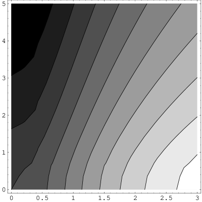
Figure 2: Contour plot of $f/f_{\rm id}$ as a function of $P_{e}=\omega_{Pe}/\omega_{Te}$ and $P_{m}=\omega_{Pm}/\omega_{Tm}$ for $k_{P}d=1$, $\omega_{Te}/\omega_{P}=0.7$, and $\omega_{Tm}/\omega_{P}=0.5$. Damping parameters are $\gamma=3.9\times 10^{-9}\omega_{P}$ and $\gamma_{e}/\omega_{Te}=\gamma_{m}/\omega_{Tm}=10^{-2}$ (these parameters are kept fixed in all simulations). Constant-force lines are plotted in steps of $\Delta f/f_{\rm id}=0.02$, starting from $f/f_{\rm id}=-0.06$ at the top left corner.

The dependence of the reduction factor $f/f_{\rm id}$ on plasma frequencies $\omega_{P\nu}$ (since $\omega_{T\nu}$ are fixed) of the magnetodielectric is illustrated in Fig. 2. Note that for this $d$, the figure actually represents the Casimir force in units $f_{0}=\pi^{2}\hbar ck_{P}^{4}/240$ ($\simeq 5.67\;{\rm kN}/{\rm m}^{2}$ for Au). One observes that the transition from the attractive to repulsive regime occurs roughly when $P_{m}>P_{e}$ and that the constant-force lines at larger $P_{m}$ and $P_{e}$ in the transition region are (nearly) straight lines characterized by a (nearly) constant ratio $P_{m}/P_{e}$. Similar behavior, however, in terms of $\varepsilon$ and $\mu$, is found for the border line between the attractive and repulsive regions in Fig. 1a of Ref.[1]. We also note that our simulation agrees with the conclusion that for large $\varepsilon$ and $\mu$ the sign and the magnitude of the force depend on the surface impedance $Z=\sqrt{\mu/\varepsilon}$ of the magnetodielectric [1]. This can be seen if we rewrite Eq. (17) in terms of the relative quantities $P_{\nu}$, $Q_{\nu}=\omega_{T\nu}/\omega_{P}$ and $\tilde{d}=k_{P}d$

$$\{\varepsilon,\mu\}=1+\frac{P^{2}_{\nu}(2Q_{\nu}\tilde{d})^{2}}{(2Q_{\nu}\tilde{d})^{2}+x\cos\phi(x\cos\phi+2Q_{\nu}\tilde{d}\gamma_{\nu}/\omega_{T\nu})}.$$ (18)

At large $P_{\nu}$ one can disregard unity here, so that $Z\sim P_{m}/P_{e}$. Accordingly, (nearly) straight lines seen in the ($P_{m},P_{e}$) contour plot correspond to constant-$Z$ lines. Since for this separation between the slabs $\varepsilon$ and $\mu$ are strongly dispersive (note that $k_{Te}d=0.7$ and $k_{Tm}d=0.5$), one must conclude that accounting for the medium dispersion does not much affect the conclusions drawn in Ref. [1] regarding the ($\varepsilon,\mu$)-dependence of the force.

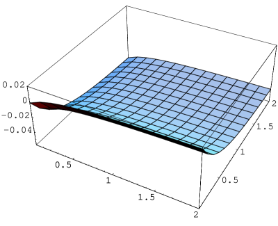
Figure 3: $f/f_{\rm id}$ as a function of $\omega_{Te}/\omega_{P}$ and $\omega_{Tm}/\omega_{P}$ for $k_{P}d=1$, $\omega_{Pe}/\omega_{Te}=0.5$, and $\omega_{Pm}/\omega_{Tm}=3$.

Clearly, of crucial importance for the appearance of the repulsive force is the relative position of the electric and magnetic resonance of the magnetodielectric. Figure 3 illustrates the variation of $f/f_{\rm id}$ with transverse frequencies ($Q_{\nu}$) of the magnetodielectric while keeping the magnitudes of $\varepsilon$ and $\mu$ (determined by $P_{\nu}$) fixed. At large $Q_{\nu}$ the force tends to a constant value because $\{\varepsilon,\mu\}\rightarrow 1+P^{2}_{\nu}$ in Eq. (18). Of course, in the opposite limit, the force vanishes as $\{\varepsilon,\mu\}\simeq 1$ for small $Q_{\nu}$. It is seen that the appearance and magnitude of the repulsive force is governed by the position of the magnetic resonance for almost all $Q_{e}$. Note that in the region where $Q_{e}>Q_{m}$, which is normally always the case, the force is attractive at this distance.

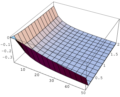
Figure 4: $f/f_{\rm id}$ as a function of the distance $k_{P}d$ between the slabs and the position $\omega_{Tm}/\omega_{P}$ of the magnetic resonance for $\omega_{Pe}/\omega_{Te}=0.5$, $\omega_{Te}/\omega_{P}=0.7$, and $\omega_{Pm}/\omega_{Tm}=3$.

Since $Q_{\nu}$ and $\tilde{d}$ appear in the form of the product $Q_{\nu}\tilde{d}=\omega_{T\nu}d/c$ in Eq. (18), the mismatch between the electric and magnetic resonances can be compensated by properly adjusting $d$ and thus one can in principle still observe the repulsive force although at larger distances. This possibility is illustrated in Fig. 4. One observes that, indeed, even for very small values of $Q_{m}$ ($\ll Q_{e}$) at larger distances there is a repulsive force between the media. To estimate the distance at which the repulsive force could be observed in a (possibly) realistic system, we note that the highest frequencies known so far at which permeabilities differ significantly from unity are (for some antiferromagnetics) in the THz range [20]. Realistic values of the parameters $Q_{\nu}$ are therefore $Q_{e}\sim 0.1$, corresponding to $\omega_{Te}$ in the range of optical frequencies, and $Q_{m}\sim 10^{-4}$, corresponding to $\omega_{Tm}$ in the THz range. The distance dependence of the (total) force for these parameters across the repulsive region is presented in Fig.5.

Figure 5: $f$ in units $10^{-14}f_{0}$ as a function of the distance $k_{P}d$ between the slabs for a ”realistic” system: $\omega_{Te}/\omega_{P}=0.1$, $\omega_{Tm}/\omega_{P}=10^{-4}$ and other parameters are the same as in Fig. 4.

As seen, the force is attractive at small distances, which supports claims made in Ref [2]. With increasing $d$, however, the effect of permeability is enforced and the force crosses over to the repulsive regime already at $k_{P}d\simeq 640$ (which is $\simeq 14{\rm\mu m}$ for Au). Thus, the effect of magnetic polarization appears at distances smaller by two orders of magnitude than it would be expected on the basis of a simple estimate $d\sim\lambda_{Tm}=2\pi\times 10^{4}\;k^{-1}_{P}$. Evidently, this effect is due to the cumulative contribution of the waves from the low-frequency side of the spectrum and is therefore a direct consequence of the medium dispersion at long wavelengths. To estimate the magnitude of the repulsive force at such distances, we calculate its largest value occurring at $k_{P}d\simeq 850$, where we find $f\simeq-2.88\times 10^{-14}f_{0}$. Accordingly, the maximal repulsive force between, e.g. Au and this hypothetical [$\omega_{Te}=0.9$ eV, $\omega_{Pe}=0.45$ eV, $\gamma_{e}=9$ meV, $\omega_{Tm}=0.9$ meV, $\omega_{Pm}=2.7$ meV, and $\gamma_{m}=9\;\mu{\rm eV}$] magnetodielectric is $f\simeq-0.16$ ${\rm nN}/{\rm m}^{2}$ and is observed at the distance $d\simeq 18.7\;{\rm\mu m}$.

Of course, at higher temperatures the above estimate becomes invalid as at such large separations between the slabs the thermal corrections must be accounted for. The force at nonzero temperature is formally obtained from Eq. (13) by letting [9] $\xi\rightarrow\xi_{m}=2\pi mk_{B}T/\hbar$ and $\int_{0}^{\infty}d\xi\rightarrow(2\pi k_{B}T/\hbar)\sum_{m=0}^{\infty}(1-\delta_{m0}/2)$, where $\xi_{m}$ are the Matsubara frequencies. One may immediately conclude that the force in the present system is always attractive at room temperature. Indeed, at $T=300$ K and for Au, the $m$th contribution to the force is governed by the quantity

$$\frac{\xi_{m}d}{c}=2\pi m\frac{k_{B}T}{\hbar\omega_{P}}k_{P}d=1.8\times 10^{-2}m\;k_{P}d.$$

Thus, at distances $k_{P}d\gtrsim 10^{2}$ only the $m=0$ term contributes as all other terms are strongly exponentially damped. Since for the Drude metals $r^{s}_{M}(0,k)=0$ [22], this term depends only on the dielectric properties of the magnetodielectric and the force is therefore attractive. We have verified this by directly calculating the force at $T=300$ K and, for example, at $k_{P}d\simeq 850$, where the zero-temperature force is maximally repulsive, we have obtained $f\simeq 5.09\times 10^{-13}f_{0}\simeq 2.89$ ${\rm nN}/{\rm m}^{2}$.

The validity of the above estimates rests upon the adequacy of the Drude (local) model for the metal adopted. This model is often used in the considerations and precise calculations of the Casimir force between metals and is generally believed to adequately describe the properties of good metals at low frequencies [17, 21]. Strictly speaking, however, the electromagnetic response of a metal is nonlocal, at least in the frequency range of the anomalous skin effect, and should therefore be described by the nonlocal reflection coefficients $r^{q}_{M}$ [11]. The effect of the metal nonlocality below $\omega<\omega_{P}$ on the Casimir force between two metal (Au) plates at zero temperature has recently been considered in detail in Ref. [23] and it has been found that anomalous skin effect produces only a minor correction (below 0.5% for $d$ above $50$ nm) to the force calculated using the local description of the metal (which also agrees with the assertion given in Ref. [21]). Moreover, as can be concluded from Fig. 9 of Ref. [23], this correction diminishes and saturates with increasing distance between the plates. Accordingly, accounting for the anomalous skin effect of the metal cannot significantly change the above estimates on the repulsive force at $T=0$ K. As follows from the small frequency behaviour of the surface impedances [23], since the property $r^{s}_{M}(0,k)=0$ holds nonlocally as well, the force at $T=300$ K is, as before, always attractive. However, since also $r^{p}_{M}(0,k)\neq 1$, contrary to the generally accepted $r^{p}_{M}(0,k)=1$, further consideration of the effect of the metal nonlocality on the Casimir force at finite temperatures is needed.

We end this short discussion by noting that very recently Henkel and Joulain reported a similar analysis [24], however, paying more attention to the dependence of the force on geometrical rather than on material parameters as we have done. In this respect, these two works are complementary. As concerns our findings on the distance dependence of the force, these are (generally) in agreement with those of Henkel and Joulain concerning thick media.

4 Summary

Using the properties of the macroscopic field operators appropriate for magnetodielectric dissipative systems, we have extended our previous approach to the Casimir effect between two dielectric multilayered stacks to magnetodielectric systems. As expected, the resulting expression for the force between the stacks is of the same form as for a purely dielectric system. However, the Fresnel coefficients are modified owing to the different magnetic properties of the system in the present case. Using this result, we have numerically analysed the effect of the medium dispersion on the Casimir force in a metal-magnetodielectric system described by the Drude-Lorentz permittivities and permeabilities. According to this analysis, taking into account the medium dispersion does not much affect the conclusions that one may draw from a simple nondispersive model of Ref. [1] regarding the material dependence of the force. Our simulations also demonstrate that the force at zero temperature in a realistic system is attractive at small distances (covering the submicron and micron range for good metals), which supports statements in Ref. [2], and, depending on the magnetic (dispersion) properties of the magnetodielectric, becomes repulsive at larger distances. However, owing to contributions of the low-frequency waves to the force, the crossover occurs at a much smaller distance than expected from the simple $d\sim\lambda_{Tm}$ estimate. At room temperature, the force on good (Drude) metals such as Au, Cu, Al remains attractive over the entire range of distances.

References

- [1] O. Kenneth, I. Klich, A. Mann, and M. Revzen, Phys. Rev. Lett. 89, 033001 (2002).
- [2] D. Iannuzzi and F. Capasso, Phys. Rev. Lett. 91, 029101 (2003).
- [3] E. M. Lifshitz, Zh. Eksp. Teor. Fiz. 29, 94 (1955) [Sov. Phys. JETP 2, 73 (1956)].
- [4] M. Bordag, U. Mohideen, and V. M. Mostepanenko, Phys. Rep. 353, 1 (2002).
- [5] O. Kenneth, I. Klich, A. Mann, and M. Revzen, Phys. Rev. Lett. 91, 029102 (2003).
- [6] Recently, Iannuzzi et al. arrived at the same conclusion in a somewhat different context; see D. Iannuzzi, M. Lisanti, and F. Capasso, Proc. Nat. Ac. Sci. USA, 101, 4019 (2004).
- [7] E. Buks and M. L. Roukes, Nature, 419, 119 (2002).
- [8] M. S. Tomaš, Phys. Rev. A 66, 052103 (2002).
- [9] C. Raabe, L. Knöll, and D.-G. Welsch, Phys. Rev. A 68, 033810 (2003); (E) ibid 69, 019901 (2004).
- [10] H. T. Dung, S. Y. Buhmann, L. Knöll, and D.-G. Welsch, Phys. Rev A 68, 043816 (2003).
- [11] L. D. Landau and E. M. Lifshitz, Electrodynamics of Continuous Media, Pergamon, Oxford, 1991.
- [12] E. M. Lifshitz and L. P. Pitaevskii, Statistical Physics, Part 2, Pergamon, Oxford, 1991, Ch. 8.
- [13] This holds only in the case of empty space between the stacks, i.e. if ; see, C. Raabe and D.-G. Welsch, Phys. Rev. A 71, 013814 (2005).
- [14] M. S. Tomaš, Phys. Rev. A 51, 2545 (1995).
- [15] H. B. G. Casimir, Porc. K. Ned. Akad. Wet. 51, 793 (1948).
- [16] R. Ruppin, Phys. Lett. A, 299, 309 (2002).
- [17] A. Lambrecht and S. Reynaud, Eur. Phys. J. D 8, 309 (2000).
- [18] V. B. Bezerra, G. L. Klimchitskaya, V. M. Mostepanenko, and C. Romero, Phys. Rev. A 69, 022119 (2004).
- [19] Numerical simulations are performed using the program Mathematica 4.2 by Wolfram Research Inc.
- [20] I. Klich, in Quantum Field Theory Under the Influence of External Conditions, QFEXT 03, edited by K. A. Milton, Rinton Press, Princeton, NJ, 2004.
- [21] I. Brevik, J. B. Aarseth, J. S. Høye, and K. A. Milton, Phys. Rev. E 71, 056601 (2005).
- [22] For a continuing discussion regarding the applicability of this result, see Refs. [18] and[21], and references therein.
- [23] R. Esquivel and V. B. Svetovoy, Phys. Rev. A 69, 062102 (2004).
- [24] C. Henkel and K. Joulain, e-print arXiv: quant-ph/0407153.