A dressing of zero-range potentials and electron-molecule scattering problem at Ramsauer-Townsend minimum

Abstract

A dressing technique is used to improve zero range potential (ZRP) model. We consider a Darboux transformation starting with a ZRP, the result of the ”dressing” gives a potential with non-zero range that depends on a seed solution parameters. Concepts of the partial waves and partial phases for non-spherical potential are used in order to perform Darboux transformation. The problem of scattering on the regular X${}_{\hbox{n}}$ and YX${}_{\hbox{n}}$ structures is studied. The results of the low-energy electron-molecule scattering on the dressed ZRPs are illustrated by model calculation for the configuration and parameters of the silane ($\hbox{SiH}_{4}$) molecule. Key words: low-energy scattering, multiple scattering, Ramsauer-Townsend minimum, silane, zero range potential.

1 Introduction

The ideas of zero range potential (ZRP) approach were recently developed $\cite[cite]{[\@@bibref{}{Balt}{}{}]},\cite[cite]{[\@@bibref{}{LY1}{}{}]},\cite[cite]{[\@@bibref{}{Der}{}{}]}$ to widen limits of the traditional treatment by Demkov and Ostrovsky [4] and Albeverio et al. [5]. The advantage of the theory is the possibility of obtaining an exact solution of scattering problem. The ZRP is conventionally represented as the boundary condition on the wave function at some point. Alternatively, the ZRP can be represented as pseudopotential (Breit $\cite[cite]{[\@@bibref{}{Breit}{}{}]},\cite[cite]{[\@@bibref{}{Der}{}{}]}$).

On the other hand, the factorization of a Schrödinger operator allows to construct in natural way exactly solvable potentials [9]. The method has the direct link to Darboux transformations (DT) theory [10]. General starting point of the theory goes up to the Matveev theorem (see e.g. [11]). The transformation can be also defined on the base of covariance property of the Schrödinger equation with respect to a transformation of wave function and potential energy.

Let us briefly describe the classical method. The DT for one-dimensional but matrix problem

$$a_{2}\frac{\partial^{2}\psi}{\partial^{2}x}+a_{1}\frac{\partial\psi}{\partial x}+a_{0}\psi=E\psi$$ (1.1)

has the form

$$\psi^{(1)}=\psi_{x}-\phi_{x}\phi^{-1}\psi,$$ (1.2)

where $\phi_{x}$ is partial derivative, $s=\phi_{x}\phi^{-1}$ is constructed by matrix (operator-valued) solution $\phi$ of the equation (1.1) for a generally different eigenvalue E’. For the matrix case it is enough to take a set of linearly independent column solutions.

The principal statement (covariance) formally yields ($\partial=\partial/\partial x$)

$$L^{(1)}\psi^{(1)}=E\psi^{(1)},\hskip 22.76219ptL^{(1)}=\sum_{n=0}^{2}a_{n}^{(1)}\partial^{n},$$ (1.3)

explicit expressions for $a_{n}^{(1)}$ are given in [12] for arbitrary order operator. We would cite here the matrix Darboux dressing formulas for the second order operator. The coefficient $a_{2}$ does not transform, so it is chosen as $a_{2}=-1/2$, while the transform for the second one generally contains the commutator

$$a_{1}^{(1)}=a_{1}+[a_{2},s],$$ (1.4)

which, for the given $a_{2}$ is zero. Finally, slightly changing the notations, the transforms are:

$$\begin{array}[]{c}\psi^{(1)}=\psi_{x}-s\psi\\ a_{0}^{(1)}=a_{0}+a_{1}^{\prime}+[a_{1},s]+2a_{2}s^{\prime}+a_{2}^{\prime}s+[a_{2},s]s=\\ a_{0}+a_{1}^{\prime}-s^{\prime},\end{array}$$ (1.5)

where commutator $[a_{1},s]=0$, and primed function is the shortcut for the derivatives by $x$. The functions $\psi^{(1)},u^{(1)}$ are often named ”dressed” ones, the auxiliary solutions of the problem (1.1) are referred as the ”prop” functions. An eigenfunction and a potential from which one starts ($\psi$ and u here) are called as the ”seed” ones. Let us mention that the proof of the Darboux covariance relation includes a link that in theory of solitons [10] is named a (general) Miura transformation that is identically solved by the substitution $"s=\phi_{x}\phi^{-1}".$ We, however, do not use this fact, going by alternative way. Notice, that in the case of the radial Schrödinger equation, $a_{1}=-1/r$, that also simplify the transform (1.5).

Darboux formulas in multi-dimensional space could be applied in the sense of Andrianov, Borisov and Ioffe ideas [14] combined with ones for the radial Schrödinger equation [10, 15]. In the circumstances, DT technique can be used so as to correct ZRP model.

We attempt to dress the ZRP by means of a special choice of DT in order to widen possibilities of the ZRP model. DT modifies the generalized ZRP (GZRP) boundary condition (Section 2) and creates a potential with arbitrarily disposed discrete spectrum levels for any angular momentum $l$. In the section 3 we consider partial waves decomposition for a wave function for a non-spherical potential so as to dress a multi-centered potential, which includes n ZRPs [6]. The problem we consider is generic: it includes a three-dimensional potential. In order to construct DT we consider some aspects of division of differential operators and use some ideas from [12]. As an important example, we consider electron scattering by the X${}_{\hbox{n}}$ and YX${}_{\hbox{n}}$ structures within the framework of the ZRP model (Section 4). In section 5 we present our calculations of the corrected by the dressing integral cross-section for the electron-silane scattering.

2 Zero range potentials and dressing

Our observation shows that generalized ZRPs (see [1]) are appear as a result of Darboux transformations. In order to demonstrate it we consider a radial Schrödinger equation for partial wave $\psi_{l}$ with orbital momentum $l$. The atomic units are used throughout the present paper $\hbar=m_{e}=1$

$$\left(-\frac{1}{2}\frac{d^{2}}{dr^{2}}-\frac{1}{r}\frac{d}{dr}+\frac{l(l+1)}{2r^{2}}+u_{l}-E\right)\psi_{l}(r)=0,$$ (2.6)

where $u_{l}$ are potentials for the partial waves with asymptotic at infinity

$$\psi_{l}(r)\sim\frac{\sin(kr-\frac{l\pi}{2}+\delta_{l})}{kr}.$$ (2.7)

The equation $(\ref{E})$ describes scattering of a particle with energy E and momentum $k=\sqrt{2E}$. In the absence of the potential, partial shifts $\delta_{l}=0$ and partial waves can be expressed via spherical functions $\psi_{l}=j_{l}(kr)$. Well known, the equations (2.6) are covariant with respect to DT (1.5) where

$$\begin{array}[]{l}a_{2}=-\frac{1}{2},\\ a_{1}=-\frac{1}{r}^{\mathstrut},\\ a_{0}=\frac{l(l+1)}{2r^{2}}^{\mathstrut}+u_{l}.\end{array}$$ (2.8)

In DT prop function $\phi$ plays an important role because one is used for calculation of $s$. The function $\phi$ is a solution of the equation $(\ref{E})$ at a particular value of energy $E=-\kappa^{2}/2$, where we assume $\kappa$ is a real number. If $\kappa$ is a complex number then dressed potential can be a complex function. In the case $u_{l}=0$ the solution $\phi$ are arbitrary combination of linearly independent solutions. Let us demonstrate that generalized ZRP can be introduced by DT. For our purpose convenient to use a chain of DTs (Crum formulas [13] with the wave and prop functions multiplied by $r$), which for our equation look like

$$\psi_{l}\rightarrow\psi_{l}^{(1)}=\hbox{const}\cdot\frac{W(r\psi_{l},r\phi_{1},\ldots,r\phi_{2l+1})}{rW(r\phi_{1},\ldots,r\phi_{2l+1})},$$ (2.9)

$$u_{l}\rightarrow u_{l}^{(1)}=u_{l}-(\ln W(r\phi_{1},\ldots,r\phi_{2l+1}))^{\prime\prime},$$ (2.10)

where $W$ is Wronskian, and $\phi_{m}$ are prop functions. The transformation $(\ref{crum})$ combines the solution $\psi_{l}$ and $2l+1$ solutions $\phi_{m}$. The Crum formulas result from the replacement of a chain of $2l+1$ first order transformations by a single ($2l+1$)th order transformation, which happens to be more efficient in practical calculations. In order to obtain ZRP we start from zero potential and use prop functions

$$\phi_{m}=h_{l}^{(1)}(\kappa_{m}r),$$ (2.11)

where $\kappa_{m}$ are solutions of the algebraical equation $\kappa_{m}^{2l+1}=\imath\alpha_{l}$. Here we assume $\alpha_{l}$ is real number. The explicit form of the spherical functions $h_{l}^{(1)}$ and some important properties of $j_{l}$ are given in the Appendix. Direct substitution of $(\ref{sms})$ to Wronskian shows that

$$W(r\phi_{1},\ldots,r\phi_{2l+1})={\rm const}.$$ (2.12)

It means that dressed potential $u_{l}^{(1)}(r>0)=0$. The transformation $(\ref{crum1})$ allows to calculate potential in range $r>0$. We state that DTs also yield a generalized ZRP at $r=0$. In order to prove this we perform transformation $(\ref{crum})$ and show that $\psi_{l}^{(1)}$ is a solution for a generalized ZRP. Since potential is equal zero in the region $r>0$, enough to determine asymptotic of the wave function. Substituting $\psi_{l}=j_{l}(kr)$ to the Crum formulas, we obtain

$$\psi_{l}^{(1)}=\hbox{const}\cdot\frac{W(rj_{l}(kr),r\phi_{1},\ldots,r\phi_{2l+1})}{rW(r\phi_{1}\ldots,r\phi_{2l+1})}\sim$$ (2.13)

$$\frac{1}{2{\rm i}}\left\{(-\imath)^{l}\frac{e^{\imath kr}}{kr}\frac{\Delta(\imath k,\kappa_{1},\ldots,\kappa_{2l+1})}{\Delta(\kappa_{1},\ldots,\kappa_{2l+1})}-\imath^{l}\frac{e^{-\imath kr}}{kr}\frac{\Delta(-\imath k,\kappa_{1},\ldots,\kappa_{2l+1})}{\Delta(\kappa_{1},\ldots,\kappa_{2l+1})}\right\},$$ (2.14)

where $\Delta$ is Wandermond determinant. Considering one as product

$$\Delta(\imath k,{\kappa}_{1},\ldots,{\kappa}_{2l+1})={\rm const}\cdot\prod_{m=1}^{2l+1}(\kappa_{m}-\imath k)$$ (2.15)

we obtain an asymptotic, which coincides with asymptotic of the solution:

$$\psi_{l}^{(1)}=\hbox{const}\cdot(h_{l}^{(1)}(kr)e^{2\imath\delta_{l}}-h_{l}^{(2)}(kr)),\hskip 19.91692pt\exp(2\imath\delta_{l})=\prod_{m=1}^{2l+1}\frac{\kappa_{m}-\imath k}{\kappa_{m}+\imath k}.$$ (2.16)

It easy to show that wave function $(\ref{Smat})$ describes a scattering by generalized ZRP with orbital momentum $l$. One is conventionally represented as the boundary condition at $r=0$ on the wavefunction. It can be verified by direct substitution to the boundary condition for generalized ZRP:

$$\left.\frac{(\frac{d}{dr})^{2l+1}\,r^{l+1}\psi_{l}^{(1)}}{r^{l+1}\psi_{l}^{(1)}}\right|_{r=0}=-\frac{2^{l}l!\alpha_{l}}{(2l-1)!!},$$ (2.17)

where $\alpha_{l}$ – inverse scattering for partial wave with orbital momentum $l$. Recall that at low-energies $\tan(\delta_{l})\sim-a_{l}k^{2l+1}$ for a short-range potential, where $a_{l}$ is scattering length. In special case of $l=0$ we obtain $(\ln r\psi)^{\prime}=-\alpha$. This generalized boundary condition can be obtained from asymptotic of the wave function in the vicinity of zero, which was used some authors [1]. Let us consider the scattering matrix on the complex $k$-plane. Each element $\exp(2\imath\delta_{l})$ has $2l+1$ poles at the points $k=\imath\kappa_{m}$, which lie on circle on the complex plane. Since the bound states correspond to the poles on the imaginary positive semi-axis on complex $k$-plane, bound state exists only if $\alpha_{l}>0$ and $l$ is odd number or if $\alpha_{l}<0$ end $l$ is even. Otherwise ZRP has an antibound state.

There is some ”generalization” of ZRP theory, then inverse scattering length in original boundary condition is replaced by ”$-k\hbox{cot}(\delta)$” (in case $l$=0). In this model, ZRP may has two (or more) bound states with non-orthogonal wave functions. This trouble does not appears in our model because our potential has only one bound state. However, we note that generalized ZRP has other trouble: bound state with orbital momentum $l>0$ does not belongs to $L^{2}$ (the zero range effect). But we think that one problem does not fatal because this model reasonably describes a low energy scattering.

Example 1: There is a simple example which proves the our observation: ZRP can be introduced by Darboux transformation. Let us consider transformation for regular solution $\psi=\sin(kr)/r$ with the prop function $\phi=\exp(\alpha r)/r$. Direct calculation yields the wave function

$$\psi^{(1)}=\hbox{const}\cdot(\psi^{\prime}-s\psi)=\frac{\sin(kr-\arctan(k/\alpha))}{kr},$$ (2.18)

which satisfies the original ZRP condition with inverse scattering $\alpha$. Repeating transformation with $\phi=\exp(-\alpha r)/r$ we obtain $\psi^{(2)}=\psi$. These example shows a relation between ZRP and DT.

Thus generalized ZRPs are appear as a result of DT. In this connexion we can raise a question about subsequent dressing of ZRP. In particular case then we deal with only one prop function $\phi$ the Crum formulas correspond to the usual DT:

$$\psi_{l}^{(1)}=\hbox{const}\cdot(\psi_{l}^{\prime}-s\psi_{l}),\hskip 22.76219pts=(\ln\phi)^{\prime},$$ (2.19)

$$u_{l}^{(1)}\equiv\displaystyle a_{0}^{(1)}-\frac{l(l+1)^{\mathstrut{}^{\displaystyle\mathstrut}}}{2r^{2}}=u_{l}+\frac{1}{r^{2}}-s^{\prime},$$ (2.20)

where we suppose potential $u_{l}$ describes ZRP. The functions $\psi_{l}$, $\phi$ are solutions of the Schrödinger equation $(\ref{E})$. Note the dressed potential $u_{l}^{(1)}$ is real for real prop function $\phi$. The next step in the dressing procedure is a definition of the free parameters of the solutions $\phi$. Since potential $u_{l}(r>0)=0$ the solution $\phi$ can be written as linear combination of spherical functions

$$\phi=Cn_{l}(\imath\kappa r)+C_{1}j_{l}(\imath\kappa r),$$ (2.21)

where $C$, $C_{1}$, $\kappa$ are parameters. The eqs. $(\ref{DT})$ allow to calculate potential in the range $r>0$, but not at $r=0$! We suppose DT yields a new zero range potential at $r=0$. In order to solve this problem consider $\phi$ in the vicinity of zero. There are two different cases. The spherical function properties show that in the case C=0 the leading term in $\phi$ is $r^{l}$ and in case C=1 one is $r^{-l-1}$. Therefore dressed coefficient $a_{0}^{(1)}$ has the following asymptotic at zero

$$\frac{l(l+1)}{2r^{2}}+u_{l}^{(1)}\sim\left\{\begin{array}[]{cl}\frac{(l+1)(l+2)}{2r^{2}}&\hbox{then \ C=0},\\ \frac{l(l-1)}{2r^{2}}^{\mathstrut{}^{\mathstrut{}^{\mathstrut}}}&\hbox{then \ C=1}.\end{array}\right.$$ (2.22)

As regards all other possible cases, it is easy to see that ones lead to the cited above cases. According to eq. $(\ref{DT2})$ dressed potential $u^{(1)}_{l}$ decreases as $\exp(-2|\kappa|r)$ at the infinity. Thus, in general DT introduces short-range core of centrifugal type (which depends on angular momentum $l$) in the potential. In this situation the boundary conditions on the dressed wavefunctions $\psi_{l}^{(1)}$ require modification. We think that in general case dressed ZRP conventionally represented as the boundary condition

$$\left.\frac{(\frac{d}{dr})^{2m+1}\,r^{m+1}\psi_{l}^{(1)}}{r^{m+1}\psi_{l}^{(1)}}\right|_{r=0}=\hbox{const},$$ (2.23)

where $m=l+1$ in case $C=0$, and $m=l-1$ then $C=1$. However, repeating DT for other values $\kappa$ and combining cases $C=0,1$ we can remove short-range core. In the absence of short-range core the boundary condition looks like eq. $(\ref{Bound})$. The chain of $N$-DT leads to new S-matrix poles, which does not depend on value $C_{1}$

$$\exp(2\imath\delta_{l}^{(N)})=\frac{(\alpha_{l}-\imath k^{2l+1})}{(\alpha_{l}+\imath k^{2l+1})}\prod_{m=1}^{N}\frac{(\kappa_{m}-\imath k)}{(\kappa_{m}+\imath k)},$$ (2.24)

Thus, we can use Darboux transformation in order to add (or remove) poles of the $S$-matrix. Changing parameter $C_{1}$ we obtain potentials with identical spectrum, called phase equivalent potentials. Such transformation is also known as isospectral deformation.

Example 2: Simplest case of $l=0$ is a instructive example. Consider original ZRP at $r=0$ with wave function $(\ref{sss})$. We can choose the solution $\phi$ as

$$\phi=\frac{\cosh(\kappa r)}{r}.$$ (2.25)

This choice corresponds the parameters $C=1$ and $C_{1}=0$. For short we omit index $l=0$. The DT $(\ref{DT})$ gives rise to the following property of the dressed wave function

$$\left.\frac{(r\psi^{(1)})^{\prime}}{r\psi^{(1)}}\right|_{r=0}=\frac{k^{2}+\kappa^{2}}{\alpha},$$ (2.26)

which slightly differs from usual boundary condition in ZRP theory $(\hbox{ln}r\psi)^{\prime}=-\alpha$. The dressed potential has the short-range tail:

$$u^{(1)}(r>0)=-\frac{\kappa^{2}}{\cosh^{2}(\kappa r)}.$$ (2.27)

Our observation shows that some partial values $C_{1}$ can give a long-range interaction, which looks like $\sim r^{-2}$.

The model we study describes the scattering of an electron on a compound particle. There were attempts to account this important circumstance by matrix potentials to be applied not only to well-known multichannel problem, but to composite particles as well [18]. The matrix is a projection of a complicated base that includes the orbital momenta, the only possible place for which is the potential if one restrict himself by the one-particle case. One could consider our proposal as an attempt to find some way in the general multi-particle space, that is especially of importance in the multicenter problem, to be studied in the next section.

3 Dressing in a multi-center problem

The principal observation allows to built a zero-range potential eigenfunction in the multi-center problem. In a more general situation one can consider a system with a smooth potential plus a number of ZRP. If one knows the Green function for the smooth potential, then one can provide a solution for the problem with the ZRPs added. This was outlined in [4], where the case of a single ZRP was considered. Generalization to the case with an arbitrary number of ZRP is straightforward. On the contrary, our general idea is to ”dress” a multicenter system without Green function consideration. This procedure gives simple formulas for partial phase and their corrections at low energies.

Let us consider scattering problem for a non-spherical potential $U$:

$$\left(-\frac{1}{2}\frac{\partial^{2}}{\partial r^{2}}-\frac{1}{r}\frac{\partial}{\partial r}+\frac{\hat{L}^{2}}{2r^{2}}+\hat{U}-E\right)\psi(\vec{r})=0,$$ (3.28)

where $\hat{L}^{2}$ is square of angular momentum operator, $E$ describes the energy of particle. The asymptotic of wave function $\psi(\vec{r})$ looks like

$$\psi(\vec{r})\stackrel{{\scriptstyle\rm r\rightarrow\infty}}{{\sim}}\exp(\imath\vec{k}\cdot\vec{r})+f(\theta)\frac{{\rm e}^{\imath kr}}{r},$$ (3.29)

where $f(\theta)$ is scattering amplitude, which depends on scattering angle $\theta$. The operator $\hat{L}^{2}$ commutes with all radial derivatives, in particular with $\partial=\partial/\partial r$. In three-dimensional space the DT may be reduced to one-dimensional matrix (or operator) problem $(\ref{E0})$ with appropriate chosen variable $x$. In our case $x=r$, functions $a_{2}$, $a_{1}$ are the same as in the section 2 and

$$a_{0}=\frac{\hat{L}^{2}}{2r^{2}}+\hat{U}.$$ (3.30)

The radial DT for any solution of Schrödinger equation is similar as in the section 2, but $s$ must be assumed as function of the operator variable $\hat{L}^{2}$. The transformation of the potential can be written as

$$\hat{U}\rightarrow\hat{U}^{(1)}=\hat{U}+\frac{1}{r^{2}}-s^{\prime}.$$ (3.31)

In order to find operator $s$ we can use covariance principal for equation $(\ref{EQU3D})$. The covariance principal $(\ref{E1})$ formally yields explicit constraint for $s$, which looks like as

$$\begin{array}[]{c}a_{0}^{\prime}+[a_{0},s]+(a_{1}s)^{\prime}+[a_{1},s]s+\{a_{2}(s^{\prime}+s^{2})\}^{\prime}+[a_{2},s](s^{\prime}+s^{2})=\\ a_{0}^{\prime}+(a_{1}s)^{\prime}+\{a_{2}(s^{\prime}+s^{2})\}^{\prime}=0^{\mathstrut{}^{\mathstrut}}.\end{array}$$ (3.32)

Integrating over $r$ we obtain operator equation for s, which in our case can be written as

$$s^{\prime}+\frac{2}{r}s+s^{2}=\frac{\hat{L}^{2}}{r^{2}}+2\hat{U}+\hbox{const},$$ (3.33)

where ”const” is some function of the operator variable $\hat{L}^{2}$, but one does not depend on r [12]. The sense of ”const” can be understood from the asymptotic behavior of s at infinity. Suppose, passage to the limit $r$ to infinity gives $s(\infty)=K(\hat{L}^{2})$ then const$=K(\hat{L}^{2})^{2}$. In principal operator $s$ can be found as series $\sum_{n=0}^{\infty}s_{n}\hat{L}^{2n}$ where coefficients $s_{n}$ depends only on $r$. It is easy to show the equation leads to recursion relations for coefficients $s_{n}$. For example, the first equation in the region where $U=0$ looks like

$$s_{0}^{\prime}+\frac{2}{r}s_{0}+s_{0}^{2}=K_{0},$$ (3.34)

where $K_{0}$ is zero coefficient in $K=\sum_{n=0}^{\infty}K_{n}\hat{L}^{2n}$. The formula $(\ref{DTU3D})$ gives non-local (over angles) potential which depends on $\hat{L}^{2}$. Thus, we have the algorithm that determine the operator $s$ and dressed potential via operator $K$. For our purpose (cross section evaluation) we need only partial phases or scattering amplitude related to operator $K$. In order to find the partial phases for dressed potential we need to apply the DT to wave function. However, we have one trouble: in general DT modifies the plane wave $\exp(\imath\vec{k}\cdot\vec{r})$. Thus, DT applied to wave function $\psi(\vec{r})$ with asymptotic $(\ref{AS3D})$ gives an another asymptotic. In some particular cases, special choose of the operator $K$ allows to avoid one problem. Indeed, consider the partial wave asymptotic for a non-spherical potential [17]

$$\psi_{J}(\vec{r})\sim\frac{1}{{2\imath kr}}(e^{\imath kr+\imath\delta_{J}}\Lambda_{J}(\vec{n})-e^{-\imath kr-\imath\delta_{J}}\Lambda_{J}(-\vec{n})),$$ (3.35)

where $\vec{n}$ is unit vector directed as $\vec{r}$, $\delta_{J}$ denote partial shifts, and $\Lambda_{J}(\vec{n})$ are normalized eigenvectors of S-matrix operator (partial harmonics). The most simple formulas for the shifts $\delta^{(1)}_{J}$ for the potential $\hat{U}^{(1)}$ result when partial harmonic $\Lambda_{J}$ are also eigenvectors of operator $K$. For example, suppose all partial harmonic $\Lambda_{J}$ are eigenvector of $K$ but only $\Lambda_{0}$ has nonzero eigenvalue $\kappa$

$$K\Lambda_{0}(\vec{n})=\kappa\Lambda_{0}(\vec{n}).$$ (3.36)

The asymptotic dressing is reduced to action of the operator $\partial-K$ on asymptotic $(\ref{as})$. It is easy to show by using expression

$$\ln\left(\frac{\kappa-{\rm i}k}{\kappa+{\rm i}k}\right)=-2{\rm i}\arctan(k/\kappa),$$ (3.37)

for real-valued variables $k$, $\kappa$, that DT changes only one partial shift $\delta_{0}$ as

$$\delta_{0}^{(1)}=\delta_{0}-\arctan(k/\kappa).$$ (3.38)

In this special case we add only one additional parameter. In the region $k\gg|\kappa|$ the second term of the equation $(\ref{delta})$ practically does not contribute to the partial cross section

$$\sigma_{J}=\frac{4\pi}{k^{2}}\sin^{2}\delta_{J}.$$ (3.39)

One makes an important contribution to the cross section when $k\approx|\kappa|$ and so one can be considered as correction at low energies.

In general case DT modifies all partial harmonics and partial shifts. DT allows to construct new solvable models with additional parameters. One of most important problems of solvable models is the problem of fitting them to some physically meaning parameters. For example, in discussed case the parameter $\kappa$ can be linked to the effective radius of the interaction or scattering length. Well known that scattering length can be defined as derivative $A=-\delta^{\prime}(k)$ at $k=0$. Considering the equation $(\ref{delta})$ at low energies we obtain ”re-normalized” scattering length

$$A^{(1)}=A+\frac{1}{\kappa}.$$ (3.40)

4 X${}_{\hbox{n}}$ and YX${}_{\hbox{n}}$ structures

For purpose of illustration we consider scattering problem for a dressed multi-center potential. The multi-center scattering within the framework of the ZRP model was investigated by Demkov and Rudakov [17] (8 centers, cube), Szmytkowski [20] (4 centers, regular tetrahedron), and others.

4.1 Electron-X${}_{\hbox{n}}$ scattering problem

Suppose structure X${}_{\hbox{n}}$ contains $n$ identical scatterers, which involve only $s$ waves. Let $R$ denote distance between two any scatterers (in points $\vec{r}_{m}$). There are three such structures in three-dimensional space - X₂, regular triangle X₃, regular tetrahedron X₄. The partial waves $\psi_{J}(\vec{r})$ and phase shifts can be classified with respect to symmetry group representation for the structures X${}_{\hbox{n}}$ (n=2,3,4), degeneracy being defined by the dimension of the representation [17]. We use the partial waves for ordinary ZRPs in general form

$$\psi(\vec{r})=\sum_{m=1}^{n}c_{m}\frac{\sin(k|\vec{r}-\vec{r}_{m}|+\delta)}{|\vec{r}-\vec{r}_{m}|}.$$ (4.41)

to derive an algebraical equation for partial phase. The s-wave boundary condition at the points $\vec{r}_{m}$ leads to an algebraical problem for a matrix $n\times n$ with compatibility condition

$$(p+(n-1)q)(p-q)^{n-1}=0,$$ (4.42)

where

$$\begin{array}[]{l}p=akR+R\tan\delta,\\ q=a(\sin(kR)+\cos(kR)\tan\delta),\\ \end{array}$$ (4.43)

From here, it is easy to show that phases satisfy the following expressions

$$\tan\delta_{J}=\left\{\begin{array}[]{cl}-a\frac{kR+(n-1)\sin(kR)}{R+(n-1)a\cos(kR)},&J=0\\ -a\frac{kR-\sin(kR)^{{}^{\mathstrut}}}{R-a\cos(kR)},&J=1,\ldots,n-1.\end{array}\right.$$ (4.44)

In special case, assuming $n=4$ we obtain the phases of a regular tetrahedron [20]. The integral cross sections $\sigma$ can be expressed as

$$\sigma=\sigma_{0}+(n-1)\sigma_{1},$$ (4.45)

where partial cross sections $\sigma_{J}$ are given by the equation $(\ref{parics})$. It is easy to link a scattering length for a molecule X${}_{\hbox{n}}$ and boundary parameter $a$. At large $R$ the parameter $a$ is reduced to a scattering length for an isolated atom. Starting from equation

$$\delta(k)=-\arctan\left(a\frac{kR+(n-1)\sin(kR)}{R+(n-1)a\,\cos(kR)}\right).$$ (4.46)

we obtain

$$A_{\rm X_{\hbox{n}}}=-\delta^{\prime}(0)=\frac{naR}{R+(n-1)a}.$$ (4.47)

Testing the result, plugging $n=1$ gives $A_{\rm X_{\hbox{n}}}=a$ for arbitrary $R$. The link (4.47) defines the monotonic function, saturated at $a\rightarrow\infty$.

4.2 Electron-YX${}_{\hbox{n}}$ scattering problem

The structures YX${}_{\hbox{n}}$ can be used, for instance, to study a slow electron scattering by the polyatomic molecules like $\hbox{H}_{2}\hbox{O}$, $\hbox{NH}_{3}$, $\hbox{CH}_{4}$, etc. For the sake of simplicity, we suppose that the scatterers X are situated in vertices of a regular structure X${}_{\hbox{n}}$. Let $D$ denotes the distance between scatterers Y-X and $R$ denotes distance between scatterers X-X. In this case, position of the scatterer Y perfectly fixed only if $n=4$ (geometric center of tetrahedron). And we have the constraint $R=2\sqrt{\frac{2}{3}}D$. The partial waves can be written as $(\ref{qwer})$, where the summation should be performed from $m=0$ to $n$. The partial phases can be derived analytically. The result is given by the expression

$$\tan\delta_{J}=-a_{\rm x}\,\frac{kR-\sin(kR)}{R-a_{\rm x}\cos(kR)},\ \ \ \ \ J=2,\ldots,n.$$ (4.48)

The $t=\tan\delta_{0,1}$ obeys the quadratic equation

$$\begin{array}[]{c}(t+a_{\rm y}k)\left(\frac{t}{n-1}+a_{\rm x}\left(\frac{k}{n-1}+\frac{\sin(kR)}{R}+t\frac{\cos(kR)}{R}\right)\right)=\\ \frac{n}{n-1}a_{\rm x}a_{\rm y}\left(\frac{\sin(kD)}{D}+t\frac{\cos(kD)}{D}\right)^{2^{\mathstrut{}^{\mathstrut}}},\end{array}$$ (4.49)

where $a_{\rm x}$, $a_{\rm y}$ denote boundary parameters. For large distances we can interpret ones parameters as scattering lengths of isolated atoms. Thus, in the limiting case when the distance $D$ is very large, the expression for $\tan\delta_{0}$ passes to first equation of $(\ref{phases_Xn})$ and $\tan\delta_{1}\sim-a_{\rm y}k$. This situation corresponds to independent scattering on a molecule X${}_{\hbox{n}}$ and an atom Y. The substitution $a_{\rm y}=0$ also reduces the $\tan\delta_{0}$ for structure YX${}_{\hbox{n}}$ to $\tan\delta_{0}$ for structure X${}_{\hbox{n}}$.

Substitution $t=-Ak$, where $A$ denotes the scattering length for a molecule YX${}_{\hbox{n}}$, and passage to the limit $k=0$ in (4.49) gives the quadratic equation, with the roots $A=0$ and

$$A_{\rm YX_{\hbox{n}}}=D\frac{(a_{\rm y}+na_{\rm x})RD+a_{\rm x}a_{\rm y}((n-1)D-2nR)}{(R+(n-1)a_{\rm x})D^{2}-na_{\rm x}a_{\rm y}R}.$$ (4.50)

The last root gives monotonic function of the atomic length $a_{\rm x}$ with the same features as in the previous section. We believe that the scattering lengths for isolated atoms do not change much if the atoms form an polyatomic molecule.

The DT discussed in Section 3 allows to correct cross sections at low energies. Thus, using the formulas $(\ref{IQ})$ and $(\ref{root})$ we obtain ”re-normalized” scattering length for a molecule YX${}_{\hbox{n}}$.

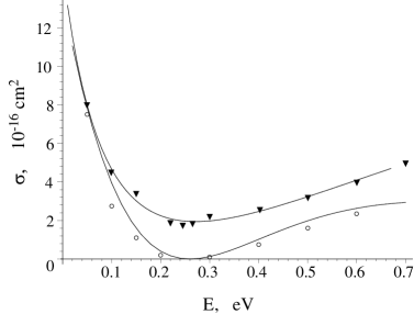
Figure 1: Integral cross sections for electron-Silane scattering around the Ramsauer-Townsend minimum; upper line - least squares fitting to the experiment [21] (triangles); lower curve describes our model calculation for partial wave ${\rm A}_{1}$; open circles denotes calculation for partial wave ${\rm A}_{1}$ [19]

5 Discussion

In this work we have presented detailed description of the new solvable models for low-energy electron-polyatomic system scattering. Now we compare our model calculations with other theoretical and experimental data. Among all possible applications we will discuss the scattering by tetrahedral molecule $\rm SiH_{\rm 4}$ (Silane) because one has most interesting point-group – symmetry group of tetrahedron. Let us focus our attention on one distinct feature of the integral cross section – Ramsauer-Townsend minimum around $\sim 0.28$ eV.

The authors of the work [19] classify the minimum as due to s-wave scattering into ${{}^{2}A_{1}}$ symmetry and attributes the main contribution to the cross section at the minimum by the p-wave scattering via $T_{2}$ component. Also they write that minimum is a result of balance of the attractive long-range and repulsive short-range interactions.

We have performed model calculation and show that Ramsauer-Townsend minimum is appeared also in consequence of balance of the attractive short-range and zero-range interactions. Our calculation is based on the formulas $(\ref{delta})$ and $(\ref{eta12})$.

In model calculation we used the following parameters (in atomic units)

$$\begin{array}[]{lll}a_{\rm x}=4.10,&R=4.51,&\kappa=0.185,\\ a_{\rm y}=1.88,&D=2.762,&\\ \end{array}$$

which are regarded as constant in the range of interest. The equilibrium distances $R$, $D$ were taken from ab initio calculation. The other parameters were chosen so as to reproduce the realistic low energy asymptotic of $\sigma$ and position of the minimum. The result of our calculation (lower curve) is shown in Figure 1. The open circles show numerical calculation [19], triangles and upper line (least squares fitting) describes the experiment [21]. Our investigation shows that ”dressing” leads to additional finite range attractive interaction, which algebraically increases the partial phase $({\delta_{0}<0})$ for partial wave ${\rm A}_{1}$ for ${\rm YX}_{4}$ structure, and causes to the deep minimum near $0.35$ eV. Thus, our partial cross sections coincide well with results other numerical data and coincide in shape with experimental data.

6 Conclusion

We introduced a class of models for electron-molecule scattering description. The principal and novel feature of the model is the dependence of effective potential on electron momentum (spherical part of Laplacian). This way we obtain more rich dependence of the scattering parameters on k, that improve a coincidence with experiment in the small energy region. It could be considered as an alternative to Demkov - Rudakov approach, with generalized partial waves introduced in each step of dressing procedure.

We write the algebraical expressions for phases of electron-X${}_{\hbox{n}}$ (and -YX${}_{\hbox{n}}$) scattering problem. We hope one can be useful to study a slow electron scattering by a molecule. We also obtain expressions for scattering lengths, which probably can be helpful for fitting of parameters (if scattering length is known). In our calculation we don’t use scattering lengths of isolated atoms, because think that boundary parameters may differ from ones.

Among the most important aspects of the paper is the demonstration of DT power as applied to multi-center scattering problem and ZRP theory. We established that ZRP can be introduced by DT. Also, these transformations allow to correct the ZRP model at low energies. As a novelty we do not use the known solution of the generalized Miura equation by eigenfuncions of the spectral matrix problem under consideration (see the Introduction) but construct particular solutions by means of operator series.

Appendix A Spherical functions properties

Below we display notations and some properties of functions used in the paper. The spherical functions $j_{l}$, $n_{l}$ are related to usual Bessel functions with half-integer indexes [7]. Ones obey the asymptotic at infinity:

$$j_{l}(kr)\sim\frac{\sin(kr-\frac{l\pi}{2})}{kr},\hskip 28.45274ptn_{l}(kr)\sim\frac{\cos(kr-\frac{l\pi}{2})}{kr}.$$ (A.51)

For our purpose, it is important that in the vicinity of zero the spherical functions have the asymptotic behavior at zero:

$$j_{l}(kr)\sim\frac{(kr)^{l}}{(2l+1)!!},\hskip 28.45274ptn_{l}(kr)\sim\frac{(2l-1)!!}{(kr)^{l+1}}.$$ (A.52)

Note the double factorial $(2l-1)!!$ satisfies the equation $(2l)!=2^{l}l!(2l-1)!!$. Also spherical functions $h_{l}^{(1,2)}$ appear in our calculations. Ones link to the functions $j_{l}$, $n_{l}$ as

$$\begin{array}[]{c}h_{l}^{(1)}(kr)=n_{l}(kr)+\imath j_{l}(kr),\\ h_{l}^{(2)}(kr)=n_{l}(kr)-\imath j_{l}(kr).\end{array}$$ (A.53)

The corresponding asymptotic can be obtained automatically. For example, at infinity

$$h_{l}^{(1)}(kr)\sim(-\imath)^{l}\,\frac{e^{{\rm i}kr}}{kr},\hskip 28.45274pth_{l}^{(2)}(kr)\sim\imath^{l}\,\frac{e^{-{\rm i}kr}}{kr}.$$ (A.54)

Refferences

References

- [1] Andreeva T G and Rudakov V S 1977 Vestnik of Leningrad Univ. 22 12-18 (in Russian); Baltenkov A S 2000 Phys. Lett. A 286 92-99
- [2] Leble S B and Yalunin S 2002 Phys. Lett. A 306 35-44; Preprint quant-ph/0205110.
- [3] Derevianko A 2003 Phys. Rev. A 67 033607
- [4] Demkov Yu N and Ostrovsky V N 1988 Zero-Range Potentials and their Applications in Atomic Physics (New York: Plenum)
- [5] Albeverio S et al 1988 Solvable Models in Quantum Mechanics (New York: Springer-Verlag)
- [6] Leble S B and Yalunin S 2003 Rad. Phys. Chem. 68 181-186
- [7] Abramowitz M and Stegun I A (ed) 1965 Handbook of mathematical functions (New York: Dover)
- [8] Breit G 1947 Phys. Rev. 71 215
- [9] Infeld L and Hull T 1951 Rev. Mod. Phys. 23 21-68
- [10] Matveev V B and Salle M A 1991 Darboux transformations and solitons (New York: Springer)
- [11] Matveev V B 1979 Lett. Math. Phys. 3 213
- [12] Zaitsev A and Leble S 1999 Preprint math-ph/9903005; 2000 Rep. Math. Phys. 46 155
- [13] Crum M M 1955 Quart. J. Math. Oxford 6 121
- [14] Andrianov A et al 1984 Phys. Lett. A 105 19-22
- [15] Schnizer W A and Leeb H 1994 J.Phys. A: Math. Gen. 27 2605-2614
- [16] Drukarev G F 1963 Theory of Collisions of electrons with Atoms (Moscow: GIZ Fiz Mat Lit) (in Russian)
- [17] Demkov Yu N and Rudakov V S 1970 Zh. Eksp. Teor. Fiz. 59 2035-2047
- [18] Sparenberg J-M and Baye D 1997 Phys. Rev. Lett. 79 3802
- [19] Jain A K et al 1987 J. Phys. B 20 389
- [20] Szmytkowski R and Szmytkowski C 1999 J. Math. Chem. 26 243-254
- [21] Wan H X et al 1989 J. Chem. Phys. 91 1340