Searching for Decoherence-Free Subspaces in Cavity Quantum Electrodynamics

Abstract

We construct a model which describes a recently performed experiment (Phys. Rev. A 64, 050301(R) (2001)) in which an entangled state between two modes of a single cavity is built. Environmental effects are taken into account and the results agree with the experimental findings. Moreover the model predicts, for different conditions of the same experiment, a decoherence-free subspace. These conditions are analyzed and slightly different experiments suggested in order to test its viability.

I Introduction

The role of environmental degrees of freedom is a central theme today both in the study of Foundations of Quantum Mechanics art1 and for technological improvement in what concerns Quantum Computation art2 . Cavity Quantum Electrodynamics art3 is one of the areas where such problem has been intensively investigated in order to establish the dynamics of the evolution of quantum superpositions considered as an open system.

Decoherence control is an important topic in this context. Systems composed by two parts interacting with a common reservoir are of interest, since theoretically they may lead to the existence of trapped states. This effect shall be associated to cross decay rate terms, which have been studied at least since Agarwall art4 . Derivations of master equations for such systems may be found in art5 ; art6 ; art7 ; art8 ; art9 and applications of them in art10 ; art11 ; art12 ; art13 .

A recent and particularly interesting experiment involves the construction of two electromagnetic field modes in a single cavity art14 . In the present contribution we investigate the consequences of a straightforward generalization of the Caldeira-Legget type model for the discussed experiment and are able to explain the results. Moreover this model predicts the existence of a decoherence-free subspace (DFS) provided the coupling to the environment satisfies certain conditions. These cannot be tested in the present experiment although with slight modifications the feasibility and robustness of such spaces can be easily accessed.

In Sec. II we present a Hamiltonian to model the system (two electromagnetic field modes) subjected to the environment, and derive a master equation in the usual Markov regime. A technique for solving this master equation, group theory for superoperators, is given in Appendix A. The experiment is described in Sec. III, where its results are compared to the theoretical ones from our model. In Sec. IV we suggest slight modifications in the experimental sketch, useful to investigate a possible tendency of forming DFS in such systems. Our conclusions are presented in Sec. V, where the feasibility of DFS is analyzed.

II From the model to the master equation

The Hamiltonian we use to describe two electromagnetic field modes in a single superconducting cavity plus environment is

$$\mathbf{H}=\mathbf{H}_{0}+\mathbf{H}_{int},$$ (1)

where

$$\mathbf{H}_{0} = \mathbf{H}_{S}+\mathbf{H}_{E},$$ (2)

$$\mathbf{H}_{S} = \hbar\Omega_{1}\mathbf{a}_{1}^{\dagger}\mathbf{a}_{1}+\hbar\Omega_{2}\mathbf{a}_{2}^{\dagger}\mathbf{a}_{2},$$

$$\mathbf{H}_{E} = \hbar\underset{k}{\sum}\omega_{k}\mathbf{c}_{k}^{\dagger}\mathbf{c}_{k},$$

$$\mathbf{H}_{int} = \underset{k}{\hbar\sum}\left(\alpha_{1k}\mathbf{a}_{1}\mathbf{c}_{k}^{\dagger}+\alpha_{1k}^{\ast}\mathbf{a}_{1}^{\dagger}\mathbf{c}_{k}\right)+\hbar\underset{k}{\sum}\left(\alpha_{2k}\mathbf{a}_{2}\mathbf{c}_{k}^{\dagger}+\alpha_{2k}^{\ast}\mathbf{a}_{2}^{\dagger}\mathbf{c}_{k}\right).$$

The operators $\mathbf{a}_{1}$ ($\mathbf{a}_{2}$) and $\mathbf{a}_{1}^{\dagger}$ ($\mathbf{a}_{2}^{\dagger}$) are annihilation and creation bosonic operators for mode $M_{a}$ ($M_{b}$) with frequency $\Omega_{1}$ ($\Omega_{2}$). The environment is modelled by a set of harmonic oscillators with creation and annihilation operators $\mathbf{c}_{k}^{\dagger}$ and $\mathbf{c}_{k}$, linearly coupled to the system, as it is usually done art15 . Harmonic oscillators are appropriate to model extended modes art16 , as phonons in the cavity mirrors and electromagnetic environment modes in the laboratory. The coupling between these environment oscillators and the oscillators of interest may occur by complicated processes art17 (e.g., a photon may be scattered from $M_{a}$ to an electromagnetic environment mode by an spurious atom inside the cavity). The coupling we considered is an effective one, related to changes of one photon between environment and system.

In what follows we deduce a master equation for the system in a similar fashion as done in Ref. art9 , where we also considered a coupling between the relevant modes (more detailed calculation can be found in Ref. art9 ). Let us take $\mathbf{\rho}\left(t\right)$ the complete density operator concerning the system plus environment. Its time evolution may be given by

$$\frac{d}{dt}\mathbf{\tilde{\rho}}\left(t\right)=\frac{-i}{\hbar}\left[\tilde{\mathbf{H}}_{int}\left(t\right),\mathbf{\tilde{\rho}}\left(t\right)\right],$$ (3)

where

$$\mathbf{\tilde{\rho}}\left(t\right)=e^{\frac{i}{\hbar}\mathbf{H}_{0}t}\mathbf{\rho}\left(t\right)e^{-\frac{i}{\hbar}\mathbf{H}_{0}t},\text{\quad\quad}e^{\frac{i}{\hbar}\mathbf{H}_{0}t}\mathbf{H}_{int}\left(t\right)e^{-\frac{i}{\hbar}\mathbf{H}_{0}t}$$

are in the interaction picture. The high quality factor of the cavity permit us to consider $\tilde{\mathbf{H}}_{int}\left(t\right)$ small, since $M_{a}$ and $M_{b}$ are weakly coupled to the environment. Disregarding the terms of third order in $\tilde{\mathbf{H}}_{int}\left(t\right)$, Eq. (3) leads to

$$\mathbf{\tilde{\rho}}\left(t\right)-\mathbf{\tilde{\rho}}\left(0\right)=-\frac{i}{\hbar}{\int_{0}^{t}}dt^{\prime}[\mathbf{\tilde{H}}_{int}\left(t^{\prime}\right),\mathbf{\tilde{\rho}}\left(0\right)]-\frac{1}{\hbar^{2}}{\int_{0}^{t}}dt^{\prime}{\int_{0}^{t^{\prime}}}dt^{\prime\prime}[\mathbf{\tilde{H}}_{int}\left(t^{\prime}\right),[\mathbf{\tilde{H}}_{int}\left(t^{\prime\prime}\right),\mathbf{\tilde{\rho}}\left(0\right)]].$$ (4)

Let us admit that at $t=0$ the system is prepared in the state $\mathbf{\rho}_{S}\left(0\right)$ and the environment is in thermal equilibrium. Thus

$$\mathbf{\tilde{\rho}}\left(0\right)=\mathbf{\rho}_{S}\left(0\right)\otimes\mathbf{\rho}_{E}\left(0\right),$$ (5)

with

$$\mathbf{\rho}_{E}\left(0\right)=\frac{1}{Z}{\prod_{k}}\exp\left(-\beta\hbar\omega_{k}\mathbf{c}_{k}^{\dagger}\mathbf{c}_{k}\right),\text{\quad\quad}Z={\prod_{k}}\sum_{n=0}^{\infty}\exp\left(-\beta\hbar\omega_{k}n\right),\text{\quad\quad}\beta=\left(k_{B}\mathcal{T}\right)^{-1}.$$ (6)

Here $k_{B}$ is Boltzmann constant, $\mathcal{T}$ is the absolute temperature and $Z$ is the partition function art18 . Taking the trace over the environment degrees of freedom in both sides of Eq. (4), we can find, in the limit of zero temperature,

$$\mathbf{\tilde{\rho}}_{S}\left(t\right)-\mathbf{\tilde{\rho}}_{S}\left(0\right) = \sum_{i,j=1}^{2}{\int_{0}^{t}}dt^{\prime}{\int_{0}^{t^{\prime}}}d\tau\left\{\left(\sum_{k}\alpha_{ik}\alpha_{jk}^{\ast}e^{i\omega_{k}\tau}\right)e^{-i\omega_{j}\tau}e^{i\left(\Omega_{j}-\Omega_{i}\right)t^{\prime}}\left(\mathbf{a}_{i}\mathbf{\tilde{\rho}}_{S}\left(0\right)\mathbf{a}_{j}^{\mathbf{\dagger}}-\mathbf{\tilde{\rho}}_{S}\left(0\right)\mathbf{a}_{j}^{\mathbf{\dagger}}\mathbf{a}_{i}\right)\right\}$$ (7)

$$+\text{h.c.},$$

where h.c. stands for Hermitian conjugate.

Notice that $\sum_{k}\alpha_{ik}\alpha_{jk}^{\ast}e^{i\omega_{k}\tau}$ decays very fast with the growing of $\tau$. Thus we may modify the integration limits above and obtain

$$\mathbf{\tilde{\rho}}_{S}\left(t\right)-\mathbf{\tilde{\rho}}_{S}\left(0\right)=\sum_{i,j=1}^{2}\left\{\begin{array}[]{c}\left(k_{ij}+i\Delta_{ij}\right)\left(\mathbf{a}_{i}\mathbf{\tilde{\rho}}_{S}\left(0\right)\mathbf{a}_{j}^{\mathbf{\dagger}}-\mathbf{\tilde{\rho}}_{S}\left(0\right)\mathbf{a}_{j}^{\mathbf{\dagger}}\mathbf{a}_{i}\right)\left({\int_{0}^{t}}dt^{\prime}e^{i\left(\omega_{j}-\omega_{i}\right)t^{\prime}}\right)\end{array}\right\}+\text{h.c.}$$ (8)

for $t\gg\tau_{c}$, where $\tau_{c}$ is the time within $\sum_{k}\alpha_{ik}\alpha_{jk}^{\ast}e^{i\omega_{k}\tau}$ have appreciable values. The constants $k_{ij}$ and $\Delta_{ij}$ are real, defined by

$$k_{ij}+i\Delta_{ij}=\sum_{k}\alpha_{ik}\alpha_{jk}^{\ast}{\int_{0}^{\tau_{c}}}d\tau e^{i\left(\omega_{k}-\Omega_{j}\right)\tau}.$$ (9)

Now we differentiate both sides of Eq. (8) and iterate to get, in an analogous way as in Ref. art19 ,

$$\frac{d}{dt}\mathbf{\tilde{\rho}}_{S}\left(t\right)=\sum_{i,j=1}^{2}\left\{\left(k_{ij}+i\Delta_{ij}\right)\left(\mathbf{a}_{i}\mathbf{\tilde{\rho}}_{S}\left(t\right)\mathbf{a}_{j}^{\mathbf{\dagger}}-\mathbf{\tilde{\rho}}_{S}\left(t\right)\mathbf{a}_{j}^{\mathbf{\dagger}}\mathbf{a}_{i}\right)e^{i\left(\Omega_{j}-\Omega_{i}\right)t}\right\}+\text{h.c.},$$ (10)

where terms of second order in $k_{ij}+i\Delta_{ij}$, that are of fourth order in $\tilde{\mathbf{H}}_{int}\left(t\right)$, were not taken into account. Returning to the Schrödinger picture we write the master equation

$$\frac{d}{dt}\mathbf{\rho}_{S}\left(t\right)=\mathcal{L}\mathbf{\rho}_{S}\left(t\right),$$ (11)

where

$$\mathcal{L} = k_{11}\left(2\mathbf{a}_{1}\bullet\mathbf{a}_{1}^{\mathbf{\dagger}}-\bullet\mathbf{a}_{1}^{\mathbf{\dagger}}\mathbf{a}_{1}-\mathbf{a}_{1}^{\mathbf{\dagger}}\mathbf{a}_{1}\bullet\right)+i\left(\Delta_{11}-\Omega_{1}\right)\left[\mathbf{a}_{1}^{\mathbf{\dagger}}\mathbf{a}_{1},\bullet\right]\mathcal{+}$$ (12)

$$k_{22}\left(2\mathbf{a}_{2}\bullet\mathbf{a}_{2}^{\mathbf{\dagger}}-\bullet\mathbf{a}_{2}^{\mathbf{\dagger}}\mathbf{a}_{2}-\mathbf{a}_{2}^{\mathbf{\dagger}}\mathbf{a}_{2}\bullet\right)+i\left(\Delta_{22}-\Omega_{2}\right)\left[\mathbf{a}_{2}^{\mathbf{\dagger}}\mathbf{a}_{2},\bullet\right]\mathcal{+}$$

$$k_{12}\left(\mathbf{a}_{1}\bullet\mathbf{a}_{2}^{\mathbf{\dagger}}+\mathbf{a}_{2}\bullet\mathbf{a}_{1}^{\mathbf{\dagger}}-\bullet\mathbf{a}_{2}^{\mathbf{\dagger}}\mathbf{a}_{1}-\mathbf{a}_{1}^{\mathbf{\dagger}}\mathbf{a}_{2}\bullet\right)+$$

$$k_{21}\left(\mathbf{a}_{2}\bullet\mathbf{a}_{1}^{\mathbf{\dagger}}+\mathbf{a}_{1}\bullet\mathbf{a}_{2}^{\mathbf{\dagger}}-\bullet\mathbf{a}_{1}^{\mathbf{\dagger}}\mathbf{a}_{2}-\mathbf{a}_{2}^{\mathbf{\dagger}}\mathbf{a}_{1}\bullet\right)+$$

$$i\left(\frac{\Delta_{12}-\Delta_{21}}{2}\right)\left(\mathbf{a}_{1}\bullet\mathbf{a}_{2}^{\mathbf{\dagger}}-\mathbf{a}_{2}\bullet\mathbf{a}_{1}^{\mathbf{\dagger}}-\bullet\mathbf{a}_{2}^{\mathbf{\dagger}}\mathbf{a}_{1}+\mathbf{a}_{1}^{\mathbf{\dagger}}\mathbf{a}_{2}\bullet\right)+$$

$$i\left(\frac{\Delta_{21}-\Delta_{12}}{2}\right)\left(\mathbf{a}_{2}\bullet\mathbf{a}_{1}^{\mathbf{\dagger}}-\mathbf{a}_{1}\bullet\mathbf{a}_{2}^{\mathbf{\dagger}}-\bullet\mathbf{a}_{1}^{\mathbf{\dagger}}\mathbf{a}_{2}+\mathbf{a}_{2}^{\mathbf{\dagger}}\mathbf{a}_{1}\bullet\right)+$$

$$i\left(\frac{\Delta_{12}+\Delta_{21}}{2}\right)\left[\mathbf{a}_{1}^{\mathbf{\dagger}}\mathbf{a}_{2}+\mathbf{a}_{2}^{\mathbf{\dagger}}\mathbf{a}_{1},\bullet\right]$$

is a Liouvillian superoperator (i.e., an operator which acts on operators). We use the conventional notation for superoperators art20 : the dot sign ($\bullet$) indicates the place to be occupied by $\mathbf{\rho}_{S}\left(t\right)$, where the superoperator acts.

In Eq. (12) the constants $k_{11}$ and $k_{22}$ are associated to the individual dissipation of the modes $M_{a}$ and $M_{b}$. The constants $\Delta_{11}$ and $\Delta_{22}$ have unitary effects, renormalizing the oscillation frequencies $\Omega_{1}$ and $\Omega_{2}$ (Lamb shifts). The coefficients $k_{12}$, $k_{21}$, $\Delta_{12}$ or $\Delta_{21}$ are related to a communication channel between the modes mediated by the environment, with unitary and non unitary effects over the evolution of the system. In Eq. (9) we see that these terms will be appreciable only if: 1) $\left|\alpha_{1k}\right|$ and $\left|\alpha_{2k}\right|$ are both not zero for several values of $k$ (this means that the system’s modes interact effectively with the same reservoir); 2) $\alpha_{1k}\alpha_{2k}^{\ast}$ have phase correlation for different $k$ (the system’s modes interact with the environment in a microscopic correlated way). Relatively large values of the cross decay terms $k_{12}+i\Delta_{12}$ and $k_{21}+i\Delta_{21}$ are important for the appearance of DFS (see Sec. IV). The experimental conditions for it will be discussed in Sec. V.

III Comparing theoretical predictions and experimental results

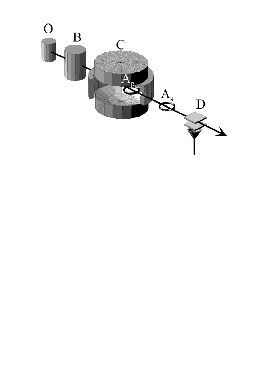
Figure 1: Sketch of the experiment (figure extracted from Ref.art14 ).

A scheme of the experiment is presented in Fig. 1. Cavity C supports two modes, $M_{a}$ and $M_{b}$, with orthogonal polarizations and different frequencies. The $M_{a}$ mode frequency is larger than that of the $M_{b}$ by $\delta$. Circular Rydberg atoms $A_{s}$ and $A_{p}$, with levels called $e$ and $g$, are sent through the cavity, the first one to create the entangled state and the second one to reveal its quantum nature. The detuning $\Delta$ between the $e\longrightarrow g$ transition frequency and the mode $M_{a}$ may be adjusted by means of the Stark effect. The sequence of the experiment is described below, closely following Ref. art14 , where all environmental effects have been ignored.

At time $t=0$, the atom $A_{s}$ enters the cavity in state $\left|e\right\rangle$. The state of the atom-two modes system is then $\left|e,0_{a},0_{b}\right\rangle$. The parameter $\Delta$ is initially set to zero and the atom interacts with $M_{a}$ through a $\frac{\pi}{2}$ Rabi pulse. The interaction with $M_{b}$ is ignored due to the detuning and the atom-field coupling is considered to be a constant (vacuum Rabi frequency $\Omega$). With an appropriate phase choice of the atomic dipole and assuming the energy of the state $\left|g,1_{a},0_{b}\right\rangle$ as zero, the atom-cavity state at $t=\frac{\pi}{2\Omega}$ will be

$$\left|\Psi\left(t=\frac{\pi}{2\Omega}\right)\right\rangle=\frac{1}{\sqrt{2}}\left[\left|e_{s},0_{a}\right\rangle+\left|g_{s},1_{a}\right\rangle\right]\left|0_{b}\right\rangle.$$

The atom is next, by Stark effect, in resonance with mode $M_{b}$ ($\Delta=-\delta$). If one now neglects the interaction with mode $M_{a}$ and takes care of the phases appropriately, one gets for $t=\frac{3\pi}{2\Omega}$

$$\left|\Psi\left(t=\frac{3\pi}{2\Omega}\right)\right\rangle=\frac{1}{\sqrt{2}}\left[e^{i\phi}\left|0_{a},1_{b}\right\rangle+\left|1_{a},0_{b}\right\rangle\right],$$ (13)

where $\phi=\frac{\pi}{2}+\frac{\pi\delta}{\Omega}$. The state ($\left|g\right\rangle$) of the atom $A_{s}$ ends up factorized and need not be considered any longer.

At time $T$ ($T>\frac{3\pi}{2\Omega}$), atom $A_{p}$ enters the cavity, whose state will be given by

$$\left|\Psi\left(t=T\right)\right\rangle=\frac{1}{\sqrt{2}}\left[i\exp\left(\frac{-i\pi\delta}{2\Omega}\right)\exp\left(i\delta T\right)\left|0_{a},1_{b}\right\rangle+\left|1_{a},0_{b}\right\rangle\right].$$

$A_{p}$ is initially in the ground state and interacts through a $\pi$ Rabi pulse with $M_{a}$. Next, it interacts with mode $M_{b}$ through a $\frac{\pi}{2}$ Rabi pulse, yielding the state

$$\left|\Psi\left(t=T+\frac{3\pi}{2\Omega}\right)\right\rangle=\frac{1}{2}\left[i\left|g_{p},1_{b}\right\rangle\left(1-e^{i\delta T}e^{i\delta\pi/2\Omega}\right)+\left|e_{p},0_{b}\right\rangle\left(1+e^{i\delta T}e^{i\delta\pi/2\Omega}\right)\right].$$

Mode $M_{a}$ ends up in the vacuum state, factorized. The probability $P_{e}(T)$ of finding $A_{p}$ in state $\left|e\right\rangle$ is therefore given by

$$P_{e}\left(T\right)=\frac{\left[1+\cos\left(\delta T+\Phi\right)\right]}{2},$$ (14)

where

$$\Phi=\frac{\delta\pi}{2\Omega}.$$

In Appendix A we present a general solution of the Master Equation (11). This may be used to describe the experiment in question taking dissipation into consideration in the period between the crossing of the two atoms. In fact, assuming that in $t=\frac{3\pi}{2\Omega}$ the cavity state is given by Eq. (13), in $t=T$, considering the interaction with the environment, will be

$$\rho_{S}\left(T\right) = \frac{1}{2}\left[\left(e^{i\phi}F_{2}\left(\tau\right)+L_{2}\left(\tau\right)\right)\left|0\right\rangle\left|1\right\rangle+\left(F_{1}\left(\tau\right)+e^{i\phi}L_{1}\left(\tau\right)\right)\left|1\right\rangle\left|0\right\rangle\right]\left[\text{h. c.}\right]$$

$$+\left(1-\frac{\left|e^{i\phi}F_{2}\left(\tau\right)+L_{2}\left(\tau\right)\right|^{2}}{2}-\frac{\left|F_{1}\left(\tau\right)+e^{i\phi}L_{1}\left(\tau\right)\right|^{2}}{2}\right)\left|0\right\rangle\left|0\right\rangle\left\langle 0\right|\left\langle 0\right|,$$

where $\tau=T-\frac{3\pi}{2\Omega}$ and

$$F_{1}\left(t\right) = \frac{1}{2}\left[\left(1-\frac{c}{r}\right)e^{\lambda_{-}t}+\left(1+\frac{c}{r}\right)e^{\lambda_{+}t}\right],$$ (15)

$$F_{2}\left(t\right) = \frac{1}{2}\left[\left(1+\frac{c}{r}\right)e^{\lambda_{-}t}+\left(1-\frac{c}{r}\right)e^{\lambda_{+}t}\right],$$

$$L_{1}\left(t\right) = \frac{1}{2}\left(\frac{k_{12}-i\Delta_{12}}{r}\right)\left(e^{\lambda_{-}t}-e^{\lambda_{+}t}\right),$$

$$L_{2}\left(t\right) = \frac{1}{2}\left(\frac{k_{21}-i\Delta_{21}}{r}\right)\left(e^{\lambda_{-}t}-e^{\lambda_{+}t}\right),$$

$$\text{\ \ \ \ \ }\lambda_{-} = -R-r,\text{ \ \ \ \ \ \ \ \ \ \ \ \ \ \ \ \ }\lambda_{+}=-R+r,$$

$$c = \frac{k_{22}-k_{11}}{2}+i\frac{\left(\Omega_{2}-\Delta_{22}\right)-\left(\Omega_{1}-\Delta_{11}\right)}{2},$$

$$r = \sqrt{c^{2}+\left(k_{12}-i\Delta_{12}\right)\left(k_{21}-i\Delta_{21}\right)},$$

$$R = \frac{k_{11}+k_{22}}{2}+i\frac{\left(\Omega_{1}-\Delta_{11}\right)+\left(\Omega_{2}-\Delta_{22}\right)}{2}.$$

Using the above solution for $\rho_{s}(T)$ it is a simple matter to evaluate $P_{e}(T)$. We get

$$P_{e}\left(T\right)=\frac{1}{4}\left|-\left(F_{1}\left(\tau\right)+e^{i\phi}L_{1}\left(\tau\right)\right)+ie^{2i\Phi}\left(e^{i\phi}F_{2}\left(\tau\right)+L_{2}\left(\tau\right)\right)\right|^{2}.$$

The maximum possible values for $\left|k_{12}\right|$, $\left|k_{21}\right|$, $\left|\Delta_{12}\right|$ and $\left|\Delta_{21}\right|$ are of the order of $k_{11}$ and $k_{22}$. Given the large detuning, the experiment is not sensitive to these cross decay constants and is consistent with $k_{12}=k_{21}=\Delta_{12}=\Delta_{21}=0$. The experimental results are also consistent with $\Delta_{11}=\Delta_{22}=0$. In this case we get

$$P_{e}\left(T\right)=\frac{1}{2}\left[\frac{e^{-2k_{11}\tau}+e^{-2k_{22}\tau}}{2}+e^{-\left(k_{11}+k_{22}\right)\tau}\cos\left(\delta T+\Phi\right)\right].$$ (16)

Making $k_{11}=k_{22}=0$, we recover expression (14).

Note that Eq. (11) has been derived for zero temperature. This is not the exact experimental condition since in thermal equilibrium the modes $M_{a}$ and $M_{b}$ contain a small fraction of thermal photons (~1). In order to take this effect into account we use effective dissipation constants for the modes $k_{11}^{ef}=\frac{\bar{n}+1}{2T_{r,a}}$ and $k_{22}^{ef}=\frac{\bar{n}+1}{2T_{r,b}}$ where $\bar{n}$ is the average number of thermal photons and $T_{r,a}$ ($T_{r,b}$) the measured decay time for mode $M_{a}$ ($M_{b}$).

There are several sources of imperfection in the experiment, related to the construction of the modes and to the atomic detection. The fidelity of the state in Eq. (13) is estimated to be of $50\%$. Therefore the interaction with the environment is not the only source of visibility loss. In order to compare our model results to the experiment we use a reduction factor of $50\%$.

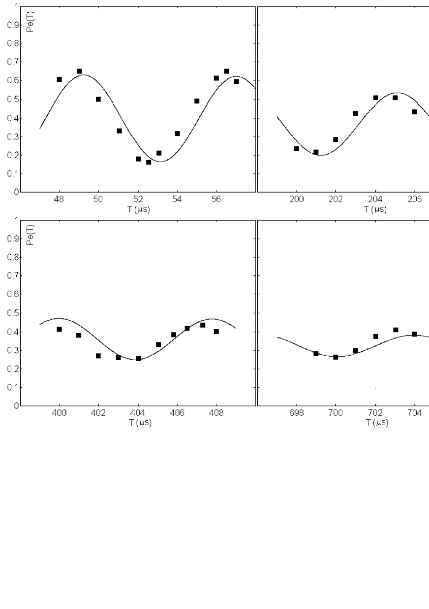
Figure 2: Probability $P_{e}(T)$ for detecting $A_{p}$ in state $e$ for the experimental situation described in Ref. art14 . The curves refer to the dissipative model. The dots are from the experiment.

In Fig. 2 we show $P_{e}(T)\times T$ for the same time windows as in Ref. art14 . Eq. (16) have been used and the experimental reduction factor was taken into account. There is good agreement between our predictions and experiment, especially in what concerns the amplitude and period of oscillation. We note a slight shift, approximately constant in all cases ($<1\mu s$), between theory and experiment. Some possible sources of this phase shift are: 1) The assumption of a constant atom-field interaction. 2) During the time of switching the atoms off resonance with mode $M_{a}$ and in resonance with mode $M_{b}$, the phase accumulation happens in a way that depends on the details of the process, not included in this model. Notice that these times are, accordingly to art14 , within $1\mu s$, ie, in the same order of the shift. 3) We have assumed that the atom interacts with just one mode at a time. The simultaneous interaction of the atom with both modes create a communication channel between the modes, which has consequences on the phase in $P_{e}(T)$. This effect may be more relevant during the switching of the atom, when the frequency of the atomic transition is not maximally far from the frequencies of $M_{a}$ and $M_{b}$.

IV Searching for decoherence-free subspaces

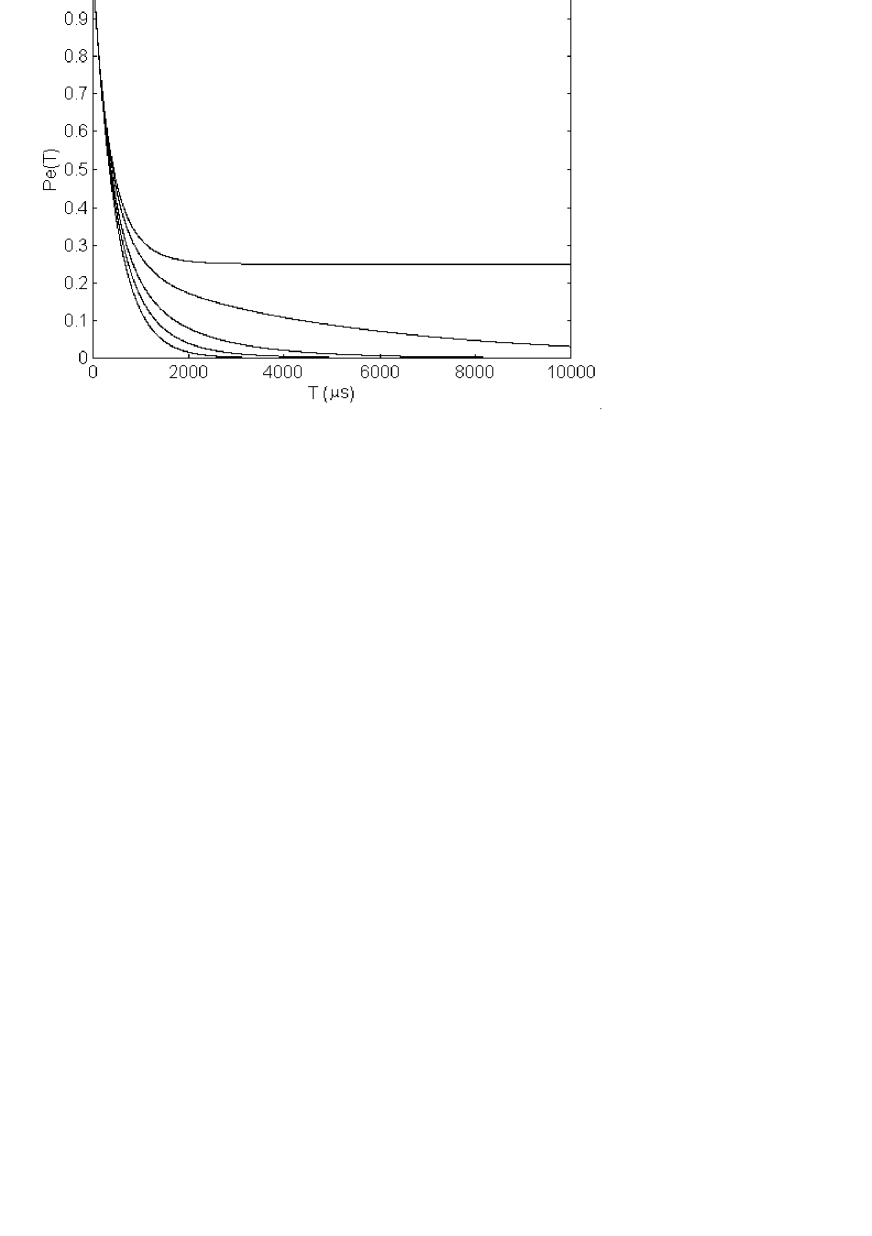
Figure 3: Probability $P_{e}(T)$ for detecting $A_{p}$ in state $e$ for resonant modes, according to the dissipative model. We consider several values for $k_{12}=k_{21}$: $k_{12}=k_{21}=0$, $k_{12}=k_{21}=0.5\sqrt{k_{11}k_{22}}$, $k_{12}=k_{21}=0.7\sqrt{k_{11}k_{22}}$, $k_{12}=k_{21}=0.9\sqrt{k_{11}k_{22}}$, $k_{12}=k_{21}=\sqrt{k_{11}k_{22}}$. Upper curves correspond to higher values for $k_{12}=k_{21}$.

We next perform a mathematical analysis of a different situation than the experimental one: let us consider resonating modes. In this case $\delta=0$ and the role of $k_{12}$ and $k_{21}$ become significant. In Fig. 3 we plot $P_{e}(T)\times T$ for the case, $\delta=0$, $k_{12}=k_{21}$ for various values of $k_{12}$, keeping the other parameters as considered in Sec. III. Notice in Fig. 3 that if $k_{12}=\sqrt{k_{11}k_{22}}$ the field in C does not go to zero for long times, suggesting a decoherence-free situation. In fact in this situation the constant $\lambda_{-}$ (Eq. (15)) has a vanishing real part and the exponentials related to it will therefore not decay. The field decay is then completely dictated by $\lambda_{+}$. So part of the field remains protected.

What does this condition $k_{12}=\sqrt{k_{11}k_{22}}$ mean physically? It means that the environment acts as a coherence feed-back mechanism. It means that photons would scatter from one mode and be transferred to the other without loosing their coherence. This may seem rather unrealistic although  it is a sound mathematical consequence of the extension of a model which works very well for a single mode art15 . Moreover, the other curves in Fig. 3 indicate that even very slight deviations from this condition already destroy the existence of this decoherence-free situation.

The experimental scheme to investigate the possibility of such an effect would need one as small as possible detuning. Of course the assembly must be altered if we don’t want the atom interacting simultaneously with both modes. We have at least two strategies:

1) In art14 a quadratic Stark effect is obtained by applying a dc voltage across the mirrors, which maintains the atomic orbital plane perpendicular to the cavity axis. In this case the atoms couple equally to both modes. We may get the Stark effect by, instead, applying two dc voltages perpendicular to the cavity axis (and perpendicular to each other). Thus the atomic orbital plane may be maintained perpendicular to the $M_{a}$ or $M_{b}$ polarizations, and the atom may be coupled to just one mode at a time. Such voltages may be produced directly in the ring around the cavity (in this case the ring must not be continuous) or, if we take away the ring, in plates outside the cavity.

2) The modes may be constructed in two separate cavities. Since we are investigating effects of the interaction between the cavities modes through the environment, it would be suitable to have the cavities as close as possible to each other. In fact, if the distance between the cavities is small in the modes’ wavelength scale, this interaction is expected to be maximized.

Adjusting the curve $P_{e}(T)$ could teach us something about the values of $k_{12}$ and $k_{21}$, or at least about a tendency to form a DFS, if one approaches the ideal limit described above.

From the theoretical point of view, it is an important issue to be able to select a specific DFS. Consider that $M_{a}$ and $M_{b}$ have the same frequency $\omega$ and

$$k_{22}+i\Delta_{22} = \kappa^{2}\left(k_{11}+i\Delta_{11}\right),$$ (17)

$$k_{12}+i\Delta_{12} = k_{21}+i\Delta_{21}=\kappa\left(k_{11}+i\Delta_{11}\right),$$

where $\kappa$ is real (a particular choice of $\kappa$ is related to the quotient between the quality factors of the modes). For all $\Delta_{ij}=0$ this is the case treated in this section when $k_{12}=k_{21}=\sqrt{k_{11}k_{22}}$. Defining the bosonic operators

$$\mathbf{A} = \frac{1}{\sqrt{1+\kappa^{2}}}\left(\mathbf{a}_{1}+\kappa\mathbf{a}_{2}\right),$$

$$\mathbf{B} = \frac{1}{\sqrt{1+\kappa^{2}}}\left(\mathbf{a}_{2}-\kappa\mathbf{a}_{1}\right),$$

we write the Liouvillian (12) as

$$\mathcal{L} = \mathcal{L}_{\mathbf{A}}+\mathcal{L}_{\mathbf{B}},$$

$$\mathcal{L}_{\mathbf{A}} = -\frac{i}{\hbar}\left(\left[\mathbf{H}_{\mathbf{A}},\bullet\right]\right)+\left(1+\kappa^{2}\right)k_{aa}\left(2\mathbf{A}\bullet\mathbf{A}^{\dagger}-\mathbf{A}^{\dagger}\mathbf{A}\bullet-\bullet\mathbf{A}^{\dagger}\mathbf{A}\right),$$

$$\mathcal{L}_{\mathbf{B}} = -\frac{i}{\hbar}\left(\left[\mathbf{H}_{\mathbf{B}},\bullet\right]\right),$$

$$\mathbf{H}_{\mathbf{A}} = \hbar\left(\omega-\Delta_{aa}\left(1+\kappa^{2}\right)\right)\mathbf{A}^{\dagger}\mathbf{A},$$

$$\mathbf{H}_{\mathbf{B}} = \hbar\omega\mathbf{B}^{\dagger}\mathbf{B}.$$

Thus, if a the system is in a state which may be written as

$$\mathbf{\rho}_{S}=\underset{m,n}{\sum}c_{m,n}\left(\mathbf{B}^{\dagger}\right)^{n}\left|0,0\right\rangle\left\langle 0,0\right|\mathbf{B}^{m}+\text{h.c.},$$ (18)

it is not affected by the environment. The states (18) define a DFS. Relevant examples for Quantum Optics and Quantum Information are the coherent state

$$\mathbf{\rho}_{S}=\left|-\kappa v\right\rangle\left|v\right\rangle\left(\text{h.c.}\right),$$

the superposition of coherent states

$$\mathbf{\rho}_{S}=N\left(\left|-\kappa v\right\rangle\left|v\right\rangle+e^{i\phi}\left|-\kappa w\right\rangle\left|w\right\rangle\right)\left(\text{h. c.}\right)$$

and the superposition of Fock states

$$\mathbf{\rho}_{S}=\frac{1}{\sqrt{1+\kappa^{2}}}\left(\left|0_{\mathbf{a}}\right\rangle\left|1_{\mathbf{b}}\right\rangle-\kappa\left|1_{\mathbf{a}}\right\rangle\left|0_{\mathbf{b}}\right\rangle\right).$$

We shall emphasize that since the conditions (17) are related to the characteristics of the environment, they can not be freely chosen by the experimenter. To understand physically what may lead to conditions (17), consider that the coupling constants of $M_{a}$ and $M_{b}$ to the reservatory modes may be factorized in the form

$$\alpha_{1k} = \alpha_{1}\gamma_{k},$$ (19)

$$\alpha_{2k} = \alpha_{2}\gamma_{k},$$

where $\alpha_{1}$ and $\alpha_{2}$ are real numbers. This corresponds to $M_{a}$ and $M_{b}$ interacting with the environment in a microscopic correlated way, with a possible difference in the intensity of the interaction art21 . For ressonant modes, conditions (19) imply conditions (17) (see Eq. (9)), and we get the DFS just described. Another way to relate conditions (19) to this DFS is to use them directly in the Hamiltonian (2) art21 . An experimental sketch to lead to this microscopic correlation would need modes as close as possible to each other, preferentialy with the same polarization, as will be discussed in more detail in the next section. If the correlation achievable in an experiment is not perfect, $k_{12}+i\Delta_{12}$ and $k_{21}+i\Delta_{21}$ will assume intermediate values between zero and the ones in (17).

V Conclusions

We deduced a master equation for two oscillators in the presence of a common reservoir and used it to model a Cavity Quantum Electrodynamics experiment involving two modes constructed in the same cavity. The theoretical results show good agreement with the experiment. Such a master equation predicts the existence of DFS if its cross terms (terms involving operators of both oscillators) have sufficiently large coefficients. Since the experiment analyzed is not sensitive to these coefficients, we proposed two slightly modificated experiments which may permit to investigate them.

The model indicates that a DFS may appear if $M_{a}$ and $M_{b}$ modes interact with the environmental modes in a microscopically correlated way. Of course it will not be the case for most systems, and it is not a simple situation to construct. Probably we may have this microscopic correlation at least partially for modes whose distance in space is small compared to the wavelength of the most important environmental modes (the ones with frequencies near the frequencies of $M_{a}$ and $M_{b}$, as may be seen in Eq. (9)). If the environment is composed mainly by electromagnetic modes, the relevant scale is the scale of the wavelengths of $M_{a}$ and $M_{b}$.

The experiment in art14 was performed with modes in the same place in space. Unfortunately it doesn’t guarantee the microscopic correlation, since $M_{a}$ and $M_{b}$ have orthogonal polarization, and then they “perceive” different microscopic environments. Although it must be not easy to built, there is no theoretical impossibility to construct modes close in the scale of their proper wavelengths.

The model states clearly that it is very difficult to achieve the parameters necessary to observe a DFS, and Fig. 3 shows how fast the DFS is spoilt when we leave the perfect situation. It is a sign that this model is realistic. But the model also indicates where are the main difficulties and what may be done to approach the ideal conditions. Due to the Cavity Quantum Electrodynamics current experimental stage, the sketches we propose may just investigate the tendency of forming DFS. If this tendency is confirmed, it shall encourage later developments.

Appendix A

Although thoroughly derived in Ref. art9 , we repeat here the solution to the master equation, with slight modifications, for completeness. We will use the parameter derivation technique, which allows one to determine coefficients $\varsigma_{i}$ such that the identity

$$e^{\left(\gamma_{1}\mathbf{O}_{1}+\gamma_{2}\mathbf{O}_{2}+\cdots+\gamma_{n}\mathbf{O}_{n}\right)t}=e^{\varsigma_{1}\left(t\right)\mathbf{O}_{1}}e^{\varsigma_{2}\left(t\right)\mathbf{O}_{2}}\cdots e^{\varsigma_{n}\left(t\right)\mathbf{O}_{n}}$$ (20)

is valid, where the $\mathbf{O}_{i}$’s are superoperators forming a closed Lie algebra and $t$ is a parameter. The parameter derivation technique consists of the following procedure:

1. Derive both sides of Eq. (20) with respect to $t$ and get

   $$\left(\sum_{i=1}^{n}\gamma_{i}\mathbf{O}_{i}\right)\exp\left(\sum_{i=1}^{n}\gamma_{i}\mathbf{O}_{i}t\right) = \dot{\varsigma}_{1}\left(t\right)\mathbf{O}_{1}\prod_{i=1}^{n}e^{\varsigma_{i}\left(t\right)\mathbf{O}_{i}}$$ (21)

   $$+\dot{\varsigma}_{2}\left(t\right)e^{\varsigma_{1}\left(t\right)\mathbf{O}_{1}}\mathbf{O}_{2}\prod_{i=2}^{n}e^{\varsigma_{i}\left(t\right)\mathbf{O}_{i}}$$

   $$+\cdots$$

   $$+\dot{\varsigma}_{n}\left(t\right)\prod_{i=1}^{n-1}e^{\varsigma_{i}\left(t\right)\mathbf{O}_{i}}\mathbf{O}_{n}e^{\varsigma_{n}\left(t\right)\mathbf{O}_{n}}.$$

2. Use the similarity transformation

   $$e^{x\mathbf{O}_{j}}\mathbf{O}_{i}e^{-x\mathbf{O}_{j}}=e^{x\left[\mathbf{O}_{j},\bullet\right]}\mathbf{O}_{i}$$ (22)

   and the linear independence of $\left\{\mathbf{O}_{i}\right\}$ in order to obtain differential equations for the parameters $\varsigma$${}_{i}\left(t\right)$.

3. Solve the $c$-numbers differential equations and obtain the factorized evolution superoperator written in the right hand side of Eq. (20).

As an example of step 2 above, let us take the second term in the r.h.s. of Eq. (21):

$$e^{\varsigma_{1}\left(t\right)\mathbf{O}_{1}}\mathbf{O}_{2} = e^{\varsigma_{1}\left(t\right)\mathbf{O}_{1}}\mathbf{O}_{2}e^{-\varsigma_{1}\left(t\right)\mathbf{O}_{1}}e^{\varsigma_{1}\left(t\right)\mathbf{O}_{1}}$$ (23)

$$= e^{\varsigma\left(t\right)\left[\mathbf{O}_{1},\bullet\right]}\mathbf{O}_{2}e^{\varsigma_{1}\left(t\right)\mathbf{O}_{1}}$$

$$\equiv f_{2}\left(\varsigma_{1}\left(t\right),\{\mathbf{O}_{i}\}\right)e^{\varsigma_{1}\left(t\right)\mathbf{O}_{1}}.$$

Analogously one can carry out a similar operation for all the other terms, define

$$f_{3}\equiv f_{3}\left(\varsigma_{1}\left(t\right),\varsigma_{2}\left(t\right),\{\mathbf{O}_{i}\}\right),\cdots,f_{n}\equiv f_{n}\left(\varsigma_{1}\left(t\right),\varsigma_{2}\left(t\right),\cdots,\varsigma_{n-1}\left(t\right),\{\mathbf{O}_{i}\}\right)$$ (24)

and write

$$\left(\sum_{i=1}^{n}\gamma_{i}\mathbf{O}_{i}\right)\exp\left(\sum_{i=1}^{n}\gamma_{i}\mathbf{O}_{i}t\right)=\left(\dot{\varsigma}_{1}\mathbf{O}_{1}+\dot{\varsigma}_{2}f_{2}+\cdots\dot{\varsigma}_{n}f_{n}\right)\exp\left(\sum_{i=1}^{n}\gamma_{i}\mathbf{O}_{i}t\right).$$ (25)

Equivalently:

$$\sum_{i=1}^{n}\gamma_{i}\mathbf{O}_{i}=\dot{\varsigma}_{1}\mathbf{O}_{1}+\dot{\varsigma}_{2}f_{2}+\cdots\dot{\varsigma}_{n}f_{n}.$$ (26)

Due to the linear independence of $\left\{\mathbf{O}_{i}\right\}$, one obtains a system of coupled differential equations for the $\varsigma_{i}$’s comparing the coefficients of each $\mathbf{O}_{i}$.

In our case we have

$$\mathbf{\rho}_{S}\left(t\right) = e^{\mathcal{L}t}\mathbf{\rho}_{S}\left(0\right)$$ (27)

$$= e^{h_{1}\left(t\right)\mathbf{a}_{1}\mathbf{\bullet a}_{1}^{\dagger}}e^{h_{2}\left(t\right)\mathbf{a}_{2}\mathbf{\bullet a}_{2}^{\dagger}}e^{z_{l}\left(t\right)\mathbf{a}_{1}\mathbf{\bullet a}_{2}^{\dagger}}e^{z\left(t\right)\mathbf{a}_{2}\mathbf{\bullet a}_{1}^{\dagger}}e^{n_{l}\left(t\right)\mathbf{\bullet a}_{1}^{\dagger}\mathbf{a}_{2}}e^{n\left(t\right)\mathbf{a}_{2}^{\dagger}\mathbf{a}_{1}\mathbf{\bullet}}$$

$$e^{m_{2}\left(t\right)\mathbf{a}_{2}^{\dagger}\mathbf{a}_{2}\mathbf{\bullet}}e^{p_{2}\left(t\right)\mathbf{\bullet a}_{2}^{\dagger}\mathbf{a}_{2}}e^{m_{1}\left(t\right)\mathbf{a}_{1}^{\dagger}\mathbf{a}_{1}\mathbf{\bullet}}e^{p_{1}\left(t\right)\mathbf{\bullet a}_{1}^{\dagger}\mathbf{a}_{1}}e^{q\left(t\right)\mathbf{a}_{1}^{\dagger}\mathbf{a}_{2}\mathbf{\bullet}}e^{q_{l}\left(t\right)\mathbf{\bullet a}_{2}^{\dagger}\mathbf{a}_{1}}\mathbf{\rho}_{S}\left(0\right).$$

Using the method just described we get

$$i\left(\Delta_{11}-\Omega_{1}\right)-k_{11} = \dot{m}_{1}\left(t\right)-n\left(t\right)\dot{q}\left(t\right)e^{m_{1}\left(t\right)-m_{2}\left(t\right)},$$

$$i\left(\Delta_{22}-\Omega_{21}\right)-k_{22} = \dot{m}_{2}\left(t\right)+n\left(t\right)\dot{q}\left(t\right)e^{m_{1}\left(t\right)-m_{2}\left(t\right)},$$

$$i\Delta_{12}-k_{12} = \dot{q}\left(t\right)e^{m_{1}\left(t\right)-m_{2}\left(t\right)},$$

$$i\Delta_{21}-k_{21} = \dot{n}\left(t\right)+n\left(t\right)\left(\dot{m}_{1}\left(t\right)-\dot{m}_{2}\left(t\right)\right)-n\left(t\right)^{2}\dot{q}\left(t\right)e^{m_{1}\left(t\right)-m_{2}\left(t\right)},$$

$$i\left(\Omega_{1}-\Delta_{11}\right)-k_{11} = \dot{p}_{1}\left(t\right)-n_{l}\left(t\right)\dot{q}_{l}\left(t\right)e^{p_{1}\left(t\right)-p_{2}\left(t\right)},$$

$$i\left(\Omega_{2}-\Delta_{22}\right)-k_{22} = \dot{p}_{2}\left(t\right)+n_{l}\left(t\right)\dot{q}_{l}\left(t\right)e^{p_{1}\left(t\right)-p_{2}\left(t\right)},$$

$$-i\Delta_{12}-k_{12} = \dot{q}_{l}\left(t\right)e^{p_{1}\left(t\right)-p_{2}\left(t\right)},$$

$$-i\Delta_{21}-k_{21} = \dot{n}_{l}\left(t\right)+n_{l}\left(t\right)\left(\dot{p}_{1}\left(t\right)-\dot{p}_{2}\left(t\right)\right)-n_{l}\left(t\right)^{2}\dot{q}_{l}\left(t\right)e^{p_{1}\left(t\right)-p_{2}\left(t\right)},$$

$$2k_{11} = z\left(t\right)\left(i\Delta_{21}-k_{21}\right)$$

$$-z_{l}\left(t\right)\left(i\Delta_{21}+k_{21}\right)+h_{1}\left(t\right)\left(-2k_{11}\right)+\dot{h_{1}}\left(t\right),$$

$$2k_{22} = z_{l}\left(t\right)\left(i\Delta_{12}-k_{12}\right)$$

$$-z\left(t\right)\left(i\Delta_{12}+k_{12}\right)+h_{2}\left(t\right)\left(-2k_{22}\right)+\dot{h_{2}}\left(t\right),$$

$$i\left(\Delta_{21}-\Delta_{12}\right)+k_{21}+k_{12} = z\left(t\right)\left(i\left(\Omega_{1}-\Delta_{11}-\Omega_{2}+\Delta_{22}\right)-k_{11}-k_{22}\right)$$

$$-h_{2}\left(t\right)\left(i\Delta_{21}+k_{21}\right)+h_{1}\left(t\right)\left(i\Delta_{12}-k_{12}\right)+\dot{z}\left(t\right),$$

$$i\left(\Delta_{12}-\Delta_{21}\right)+k_{12}+k_{21} = z_{l}\left(t\right)\left(i\left(\Omega_{2}-\Delta_{22}-\Omega_{1}+\Delta_{11}\right)-k_{22}-k_{11}\right)$$ (28)

$$-h_{1}\left(t\right)\left(i\Delta_{12}+k_{12}\right)+h_{2}\left(t\right)\left(i\Delta_{21}-k_{21}\right)+\dot{z_{l}}\left(t\right).$$

The solution reads

$$n\left(t\right) = \frac{L_{2}\left(t\right)}{F_{1}\left(t\right)},\quad\quad q\left(t\right)=\frac{L_{1}\left(t\right)}{F_{1}\left(t\right)},$$

$$e^{m_{1}\left(t\right)} = F_{1}\left(t\right),\quad\quad e^{m_{2}\left(t\right)}=e^{-2Rt}e^{-m_{1}\left(t\right)},$$

$$h_{1}\left(t\right) = \left(\left|F_{2}\left(t\right)\right|^{2}+\left|L_{2}\left(t\right)\right|^{2}\right)e^{4k_{m}t}-1,$$

$$h_{2}\left(t\right) = \left(\left|F_{1}\left(t\right)\right|^{2}+\left|L_{1}\left(t\right)\right|^{2}\right)e^{4k_{m}t}-1,$$

$$z\left(t\right) = -\left(L_{1}\left(t\right)F_{2}^{\ast}\left(t\right)+L_{2}^{\ast}\left(t\right)F_{1}\left(t\right)\right)e^{4k_{m}t},$$

$$z_{l}\left(t\right) = z^{\ast}\left(t\right),$$

$$n_{l}\left(t\right) = \left(n\left(t\right)\right)^{\ast},\quad\quad q_{l}\left(t\right)=\left(q\left(t\right)\right)^{\ast},$$

$$p_{2}\left(t\right) = \left(m_{2}\left(t\right)\right)^{\ast},\quad\quad p_{1}\left(t\right)=\left(m_{1}\left(t\right)\right)^{\ast},$$ (29)

where $F_{1}\left(t\right)$, $F_{2}\left(t\right)$, $L_{1}\left(t\right)$ and $L_{2}\left(t\right)$ are given by Eqs. (15).