Stabilizing qubit coherence via tracking-control

Abstract

We consider the problem of stabilizing the coherence of a single qubit subject to Markovian decoherence, via the application of a control Hamiltonian, without any additional resources. In this case neither quantum error correction/avoidance, nor dynamical decoupling applies. We show that using tracking-control, i.e., the conditioning of the control field on the state of the qubit, it is possible to maintain coherence for finite time durations, until the control field diverges.

I Introduction

Protecting quantum coherence in the presence of decoherence due to coupling to an uncontrollable environment is an important goal of quantum control, with applications in, e.g., quantum information processing Nielsen:book , and coherent control Brumer:book . Various methods have been developed for this purpose, e.g., quantum error correcting codes Steane:99 , decoherence-free subspaces LidarWhaley:03 , and dynamical decoupling Viola:01a , and combinations thereof ByrdWuLidar:review . However, none of these methods is applicable in the simplest possible case of interest, of a single qubit subject to Markovian decoherence: both quantum error correcting codes and decoherence-free subspaces rely on an encoding of the state of the qubit into the state of several qubits, whereas dynamical decoupling is inapplicable in the fully Markovian regime, since it is effectively equivalent to the quantum Zeno effect Facchi:03 , i.e., requires in an essential manner that the bath retains some memory of its interaction with the system.

In this work we show that tracking-control is capable of stabilizing the coherence of a single qubit subject to Markovian decoherence. Tracking-control has a rich history in classical control theory Hirschorn:79 ; Hirschorn:81 ; Hirschorn:88 ; Jakubczyk:93 ; Retchkiman:95 . It was extensively studied by Rabitz and co-workers in the context of closed quantum systems (specifically, molecular systems) Chen:95 ; Lu:95 ; Gross:93 ; Zhu:99 ; Zhu:98 ; Zhu:03 . Here it refers to the instantaneous adjustment of the control field based on a continuous measurement of the state of the qubit. This is, of course, a very strong assumption, which may be appropriate for classical control, but cannot be satisfied in principle if non-commuting quantum observables are involved. It turns out that we are able to overcome this obstacle by choosing a specific form for our control fields, as explained in detail below. In general, one can envision performing quantum tracking control based on the incomplete information gleaned in real-time from measuring an as large as possible set of commuting observables. It is an open problem to estimate the quality of the (partial) tracking one can thus attain.

The tracking solution we find in our case becomes singular after a finite time (i.e., the control fields diverge). Such singularities are a well-known feature of tracking control Chen:95 ; Lu:95 ; Gross:93 ; Zhu:99 , and can in some cases be removed Zhu:99 . We analyze the nature of the singularity occurring in our case, finding that is is unavoidable.

A related control problem was recently addressed by Belavkin and co-workers in Ref. Bouten:04 , using the quantum filtering (or stochastic master) equation Belavkin:80 . In their work the control objective is to take a qubit from an unknown initial state to the $|0\rangle$ state. In this approach one naturally accounts for the unavailability of complete information from the measurement process (using filtering), but the resulting quantum Bellman-Hamilton-Jacobi equation is very hard to solve even for a qubit, unless one makes drastic simplifying assumptions about the control field.

Purely unitary control in the presence of decoherence has also been addressed by Recht et al. in Ref. Recht:02 . It was shown there that in the case of so-called relaxing semigroups (quantum dynamical semigroups Alicki:87 with a unique fixed point), one can control the equilibrium state of the dynamics. Relaxing semigroups are in fact a case that is orthogonal to the case we study here, as they involve non-unital channels, while we study only unital channels. These issues are clarified below.

Finally, the problem of coherent control of a qubit subject to Markovian dynamics has been studied in detail by Altafini, using a Lie algebraic framework Altafini:03 ; Altafini:04 . This work has elucidated the corresponding conditions for accessibility, small- and finite-time controllability, using the coherence vector representation Alicki:87 and employing classical control-theory notions.

The structure of the present paper is as follows. In the next Section we define the model of a single qubit subject to Markovian decoherence, and define our control objectives in terms of the purity and coherence. In Sec. III we set up the coherence tracking problem and solve it explicitly for a qubit subject to pure dephasing. In Sec. IV we discuss the generality of this result by defining equivalence classes of the pure dephasing channel to which our coherence-tracking solution also applies. In Sec. V we discuss the nature of the singularity of our control fields, and show that this singularity cannot be avoided. We conclude in Sec. VI with a brief summary and a list of open questions inspired by this work.

II Model and Objectives

II.1 Purity

We consider a single qubit subject to Markovian decoherence and controlled via a control Hamiltonian $H$. Then the system dynamics is governed by a master equation of the form

$$\frac{\partial\rho}{\partial t}=-\frac{i}{\hbar}[H,\rho]+{\mathcal{L}}(\rho),$$ (1)

where the Lindbladian is

$${\mathcal{L}}(\rho)=\frac{1}{2}\sum_{i,j}a_{ij}\left([F_{i},\rho F_{j}^{\dagger}]+[F_{i}\rho,F_{j}^{\dagger}]\right),$$ (2)

where the matrix $A=(a_{ij})$ is positive semidefinite [ensuring completely positivity of the mapping ${\mathcal{L}}(\rho)$], and where the Lindblad operators $\{F_{i}\}$ are the coupling operators of the system to the bath Alicki:87 . One can always diagonalize $A$ using a unitary transformation $W=(w_{ij})$ and define new Lindblad operators $G_{i}=\sum w_{ij}F_{j}$ such that

$${\mathcal{L}}(\rho)=\frac{1}{2}\sum_{i}\gamma_{i}\left([G_{i},\rho G_{i}^{\dagger}]+[G_{i}\rho,G_{i}^{\dagger}]\right),$$ (3)

where $\gamma_{i}\geq 0$ are the eigenvalues of $A$.

In such a Markovian system it is impossible to control the purity

$$p\equiv\mathrm{Tr}(\rho^{2})$$ (4)

of a state $\rho$ in such a way so as to maintain it at its initial value Ketterle:92 ; Tannor:99 . To see this note that the time derivative of $p$ is given by

$$\frac{\partial p}{\partial t} = \frac{\partial\mathrm{Tr}(\rho^{2})}{\partial t}=2\mathrm{Tr}(\rho\dot{\rho})$$ (5)

$$= -\frac{2i}{\hbar}\underbrace{\mathrm{Tr}(\rho[H,\rho])}_{=0}+2\mathrm{Tr}(\rho{\mathcal{L}}(\rho)),$$

where we used cyclic invariance under the trace. Thus the Hamiltonian control term cannot change the first derivative of the purity, and hence cannot keep it at its initial value. This is also known as the “no-cooling principle”.

Moreover, for certain Lindbladians purity is a strictly decreasing function under the Markovian semigroup dynamics. This is the case for all unital Lindbladians, i.e., those for which ${\mathcal{L}}(I)=0$ (e.g., Altafini:04 ). In this case one finds from Eq. (3) that $\sum_{i}\gamma_{i}\left(G_{i}G_{i}^{\dagger}-G_{i}^{\dagger}G_{i}\right)=0$. Thus a sufficient condition for unitality is that the $G_{i}$ are normal (e.g., unitary): $G_{i}G_{i}^{\dagger}=G_{i}^{\dagger}G_{i}$. Subject to normality it is possible give a simple proof of the monotonic decrease of $p$:

$$\frac{\partial p}{\partial t} = 2\mathrm{Tr}(\rho{\mathcal{L}}(\rho))$$

$$= \sum_{i}\gamma_{i}\mathrm{Tr}\{\rho\left([G_{i},\rho G_{i}^{\dagger}]+[G_{i}\rho,G_{i}^{\dagger}]\right)\}$$

$$= 2\sum_{i}\gamma_{i}\{\mathrm{Tr}(X_{i}Y_{i})-\frac{1}{2}[\mathrm{Tr}(X_{i}X_{i}^{\dagger})+\mathrm{Tr}(Y_{i}Y_{i}^{\dagger})]\},$$

where $X_{i}=\rho G_{i}$ and $Y_{i}=\rho G_{i}^{\dagger}$, and we used $\rho=\rho^{{\dagger}}$. Now apply the arithmetic-geometric mean inequality for matrices, $\left\|XY\right\|\leq\frac{1}{2}(\left\|X^{\dagger}X+YY^{\dagger}\right\|)$, where $\left\|\cdot\right\|$ is any unitarily-invariant norm (such as $\mathrm{Tr}$) Bhatia:book [p.263]. Also, $\left\|X^{\dagger}X+YY^{\dagger}\right\|\leq\left\|X^{\dagger}X\right\|+\left\|YY^{\dagger}\right\|$. Then:

$$\mathrm{Tr}(X_{i}Y_{i})-\frac{1}{2}[\mathrm{Tr}(X_{i}X_{i}^{\dagger})+\mathrm{Tr}(Y_{i}Y_{i}^{\dagger})] \leq \frac{1}{2}[\mathrm{Tr}(X_{i}^{\dagger}X_{i}+Y_{i}Y_{i}^{\dagger})]-\frac{1}{2}[\mathrm{Tr}(X_{i}X_{i}^{\dagger})+\mathrm{Tr}(Y_{i}Y_{i}^{\dagger})]$$ (6)

$$\leq 0.$$

Thus, using $\gamma_{i}\geq 0$, we have $\frac{\partial p}{\partial t}\leq 0$. Purity in the case of unital Lindbladians is, therefore, a strictly decaying function under Hamiltonian control. This conclusion is unchanged even with feedback, namely, even if the Hamiltonian includes dependence on the qubit state, i.e., if $H=H[\rho]$. The situation is different for non-unital Lindbladians Recht:02 ; Altafini:04 . These channels can increase the purity even without active control. E.g., under spontaneous emission an arbitrary qubit mixed-state is gradually purified to $|0\rangle$. In this work we consider only unital Lindbladians.

II.2 Coherence

Another quantum quantity of relevance is coherence, i.e., the off-diagonal elements of $\rho$. This is, of course, a basis-dependent quantity (it is not invariant under unitary transformations), so that in what follows we assume that one has fixed a basis for physical reasons (e.g., there is a magnetic field pointing in the $z$ direction, or there is a pure dephasing type coupling to the bath, represented by a $\sigma_{z}$-Lindblad operator). We will show that tracking control is capable of stabilizing the coherence of a single qubit. A qubit is completely characterized by its density matrix

$$\rho=\left(\begin{array}[]{cc}\rho_{00}&\rho_{01}\\ \rho_{10}&\rho_{11}\end{array}\right),$$ (7)

with the additional constraints $\mathrm{Tr}(\rho)=1$, $\rho_{10}=\rho_{01}^{\ast}$ and $\mathrm{Tr}(\rho^{2})\leq 1$. We follow the approach in Alicki:87 and parametrize $\rho$ using the Bloch vector $\vec{v}$ with the real components

$$v_{\alpha}=\frac{1}{2}\mathrm{Tr}(\rho\sigma_{\alpha}),$$ (8)

where $\sigma_{\alpha}$, $\alpha\in\{x,y,z\}$, are the Pauli matrices, and we identify the Lindblad operators as $F_{1}=\sigma_{x},F_{2}=\sigma_{y},F_{3}=\sigma_{z}$. We then have

$$\rho=\frac{1}{2}{(I}+\vec{v}\cdot\vec{\sigma}).$$ (9)

The purity $p$ is then given by the Bloch sphere radius,

$$p=v_{x}^{2}+v_{y}^{2}+v_{z}^{2},$$ (10)

while the coherence $c$ between levels $|0\rangle$ and $|1\rangle$ is given by the radius in the $x-y$ plane,

$$c=v_{x}^{2}+v_{y}^{2}.$$ (11)

Our objective is to have $c$ be constant during the evolution. Thus we impose the following constraint:

$$\frac{1}{2}\frac{\partial c}{\partial t} = v_{x}\dot{v}_{x}+v_{y}\dot{v}_{y}$$ (12)

$$= 0.$$

III Tracking Control of Coherence

III.1 Tracking equation

Noticing that the traceful part (reference energy) of the control Hamiltonian drops out of the commutator $[H,\rho]$ we expand $H$ in the traceless Pauli basis:

$$H=\frac{\hbar}{2}(\omega_{0}(t)\sigma_{z}+\omega_{1}(t)\sigma_{x}-\omega_{2}(t)\sigma_{y})$$ (13)

We wish to solve for the control fields $\omega_{i}(t)$ so that the coherence constraint (12) is satisfied. Note that we are assuming that the intrinsic system Hamiltonian either vanishes, or that we are working in the rotating frame with respect to this Hamiltonian.

Substituting this and the expansion (9) into the Lindblad equation (1), and using trace-orthonormality of the Pauli matrices, we obtain the generalized Bloch equations

$$\dot{v}_{x}(t) = -\gamma_{3}v_{x}(t)+(\alpha-\omega_{0}(t))v_{y}(t)+(\beta-\omega_{2}(t))v_{z}(t)-2\lambda,$$ (14)

$$\dot{v}_{y}(t) = (\alpha+\omega_{0}(t))v_{x}(t)-\gamma_{2}v_{y}(t)+(\delta-\omega_{1}(t))v_{z}(t)-2\mu,$$ (15)

$$\dot{v}_{z}(t) = (\beta+\omega_{2}(t))v_{x}(t)+(\delta+\omega_{1}(t))v_{y}(t)-\gamma_{1}v_{z}(t)-2\nu.$$ (16)

Here we identify the parameters from Eqs. (14)-(16) with the $a_{ij}$ from Eq. (2) as follows:

$$\gamma_{1} = 2(a_{22}+a_{33}),\quad\gamma_{2}=2(a_{11}+a_{33}),\quad\gamma_{3}=2(a_{11}+a_{22})$$ (17)

$$\alpha = 2\mathrm{Re}(a_{12}),\quad\beta=2\mathrm{Re}(a_{13}),\quad\delta=2\mathrm{Re}(a_{23})$$ (18)

$$\lambda = \mathrm{Im}(a_{23}),\quad\mu=-\mathrm{Im}(a_{13}),\quad\nu=\mathrm{Im}(a_{12})$$ (19)

Note from Eqs. (14-16) that the $\gamma_{i}$ can be interpreted as damping coefficients, while $\alpha,\beta$ and $\delta$ play the role of Lamb shifts (modify the control fields), and $\lambda,\mu$ and $\nu$ are the coordinates of an affine shift of the Bloch vector (which plays a role, e.g., in spontaneous emission). Positive semi-definiteness of $A=(a_{ij})$ imposes various conditions on these parameters Alicki:87 .

In matrix form Eqs. (14-16) can be written as an affine linear transformation

$$\dot{\vec{v}}(t)=(M_{0}+M(t))\vec{v}(t)+\vec{k},$$ (20)

where the decoherence is affected by

$$M_{0} = \left(\begin{array}[]{ccc}-\gamma_{3}&\alpha&\beta\\ \alpha&-\gamma_{2}&\delta\\ \beta&\delta&-\gamma_{1}\end{array}\right),$$ (24)

$$\vec{k} = -2(\lambda,\mu,\nu)^{t},$$ (25)

(superscript $t$ denotes transpose) and the control Hamiltonian is represented by the real, antisymmetric matrix

$$M(t) = \left(\begin{array}[]{ccc}0&-\omega_{0}(t)&-\omega_{2}(t)\\ \omega_{0}(t)&0&-\omega_{1}(t)\\ \omega_{2}(t)&\omega_{1}(t)&0\end{array}\right)$$ (29)

$$= \sum_{j=0}^{2}\omega_{j}(t)\Lambda_{j},$$ (30)

where the matrices

$$\Lambda_{0}=\left(\begin{array}[]{ccc}0&-1&0\\ 1&0&0\\ 0&0&0\end{array}\right),\quad\Lambda_{1}=\left(\begin{array}[]{ccc}0&0&0\\ 0&0&-1\\ 0&1&0\end{array}\right),\quad\Lambda_{2}=\left(\begin{array}[]{ccc}0&0&-1\\ 0&0&0\\ 1&0&0\end{array}\right)$$ (31)

close as an $\mathrm{so}(3)$ subalgebra of $\mathrm{su}(3)$ (we use a slightly different convention for the signs than the standard one Cornwell:84II ):

$$[\Lambda_{0},\Lambda_{1}]=-\Lambda_{2},\quad[\Lambda_{1},\Lambda_{2}]=-\Lambda_{0},\quad[\Lambda_{2},\Lambda_{0}]=-\Lambda_{1}.$$ (32)

Solving Eq. (15) for $\omega_{1}(t)$ and Eq. (14) for $\omega_{2}(t)$ we obtain

$$\omega_{1}(t) = \frac{(\alpha+\omega_{0}(t))v_{x}(t)-\gamma_{2}v_{y}(t)+\delta v_{z}(t)-2\mu-\dot{v}_{y}(t)}{v_{z}(t)},$$ (33)

$$\omega_{2}(t) = \frac{-\gamma_{3}v_{x}(t)+(\alpha-\omega_{0}(t))v_{y}(t)+\beta v_{z}(t)-2\lambda-\dot{v}_{x}(t)}{v_{z}(t)}.$$ (34)

Substituting this into Eq. (16) and using the imposed constraint of constant coherence, $\dot{c}=0$, we find a non-linear first-order differential equation for $v_{z}(t)$ given by

$$\dot{v}_{z}(t)=F(t)+\frac{G(t)}{v_{z}(t)}-\gamma_{1}v_{z}(t),$$ (35)

where we have defined

$$F(t) \equiv 2\beta v_{x}(t)+2\delta v_{y}(t)-2\nu,$$ (36)

$$G(t) \equiv -\gamma_{3}v_{x}^{2}(t)-\gamma_{2}v_{y}^{2}(t)+2\alpha v_{x}(t)v_{y}(t)-2\lambda v_{x}(t)-2\mu v_{y}(t).$$ (37)

Eq. (35) is our tracking equation.

III.2 Solution of the tracking equation in the case of pure dephasing

We first consider the relatively simple case of diagonal $A$ (which implies that $\alpha=\beta=\delta=\lambda=\mu=\nu=0$), with equal damping along the $x$ and $y$ axes ($\gamma_{2}=\gamma_{3}\equiv\gamma$), and $\gamma_{1}=0$. This is the case known as pure dephasing (see below), and is generalized in Section IV. The Bloch equations then become:

$$\frac{\partial\vec{v}}{\partial t} = \left(\begin{array}[]{ccc}-\gamma&-\omega_{0}(t)&-\omega_{2}(t)\\ \omega_{0}(t)&-\gamma&-\omega_{1}(t)\\ \omega_{2}(t)&\omega_{1}(t)&0\end{array}\right)\vec{v}$$ (41)

$$= \vec{\Omega}(t)\times\vec{v}(t)+\vec{\Gamma}\cdot\vec{v}(t),$$ (42)

where

$$\vec{\Omega}(t) = (\omega_{1}(t),-\omega_{2}(t),\omega_{0}(t)),$$

$$\vec{\Gamma} = (-\gamma,-\gamma,0).$$ (43)

The vector $\vec{\Omega}$ acts as an effective time-dependent magnetic field and rotates the coherence vector in a manner designed (see below) to keep the coherence constant for as long as possible.

III.2.1 Uncontrolled (free) dynamics

Under free evolution (uncontrolled scenario: $H=0$) the system dynamics is governed by Markovian decoherence, subject to a master equation of the form

$$\frac{\partial\rho}{\partial t}=-\frac{i}{\hbar}[H,\rho]+\frac{\gamma}{2}\left(\sigma_{z}\rho\sigma_{z}-\rho\right),$$ (44)

or, equivalently, to the following Bloch equations [Eq. (42)]:

$$\dot{v}_{x}(t)=-\gamma v_{x}(t),~{}\dot{v}_{y}(t)=-\gamma v_{y}(t),~{}\dot{v}_{z}(t)=0.$$ (45)

The solution is

$$v_{x}(t) = \exp[-\gamma t]v_{x}(0),$$

$$v_{y}(t) = \exp[-\gamma t]v_{y}(0),$$

$$v_{z}(t) = v_{z}(0).$$ (46)

This is known as pure dephasing, or a phase-flip channel Nielsen:book , since in the corresponding Kraus operator-sum representation

$$\rho(t) = \left(\begin{array}[]{cc}\rho_{00}&e^{-\gamma t}\rho_{01}\\ e^{-\gamma t}\rho_{01}^{\ast}&1-\rho_{00}\end{array}\right)$$ (49)

$$= (1-a)I\rho I+a\sigma_{z}\rho\sigma_{z},$$ (50)

the qubit undergoes a phase flip with probability $a=(1-e^{-\gamma t})/2$ ($I$ is the identity matrix).

III.2.2 Controlled dynamics

Eqs. (35)-(37) simplify considerably in the pure dephasing case, and using the expression $c=v_{x}^{2}+v_{y}^{2}$ (is constant) for the coherence we find from Eq. (35):

$$\dot{v}_{z}(t)=\frac{-\gamma c}{v_{z}(t)}.$$ (51)

Multiplying by $v_{z}(t)$ and integrating $\frac{1}{2}d(v_{z}(t))^{2}/dt$, the solution is

$$v_{z}(t)=\left(\pm\right)\sqrt{-2\gamma ct+v_{z}^{2}(0)}.$$ (52)

It is clear that $v_{z}(t)$ does not stay real for times $t>t_{b}$ where

$$t_{b}=\frac{v_{z}^{2}(0)}{2\gamma c}.$$ (53)

What happens is that $v_{z}(t_{b})=0$, so that purity equals coherence. Since the control fields trade decrease in purity in return for stabilization of coherence, at the breakdown point this trade-off becomes impossible. Mathematically, the constraint $\dot{c}=0$ forces the control fields to diverge. We further investigate the implications of this breakdown below.

We can solve for the corresponding control fields from Eqs. (33),(34), yielding

$$\omega_{2}(t) = \left(\pm\right)\frac{-\gamma v_{x}(t)-\omega_{0}(t)v_{y}(t)-\dot{v}_{x}}{\sqrt{-2\gamma ct+v_{z}^{2}(0)}},$$ (54)

$$\omega_{1}(t) = \left(\pm\right)\frac{\omega_{0}(t)v_{x}(t)-\gamma v_{y}(t)-\dot{v}_{y}(t)}{\sqrt{-2\gamma ct+v_{z}^{2}(0)}}.$$ (55)

Note that the field $\omega_{0}(t)$ can be chosen arbitrarily. Also note that the fields $\omega_{1}(t),\omega_{2}(t)$ depend on $v_{x}(t)$ and $v_{y}(t)$. This is why the method is called “tracking control”: the control strategy depends on the instantaneous state of the system we desire to control. This can be technically highly demanding, since it implies the ability to make very fast measurements (i.e., much faster than the decoherence time-scale), combined with classical processing to solve for the control fields and real-time feedback. Nevertheless, recent cavity-QED experiments haven demonstrated the possibility of such real-time feedback control Steck:04 . For a quantum-mechanical system such as a qubit, tracking control involves an intrinsically undesirable feature: simultaneous knowledge of $v_{x}(t)$ and $v_{y}(t)$ is impossible since $\sigma_{x}$ and $\sigma_{y}$ are non-commuting observables. However, there is a simple fix for this problem, once we realize that the time dependence of $v_{x}(t)$ and $v_{y}(t)$ is itself induced by the control fields. Thus, we can use fields that fix $v_{x}(t)=v_{x}(0)$ and $v_{y}(t)=v_{y}(0)$, which is, of course, just a particular way of keeping the coherence $c=v_{x}^{2}+v_{y}^{2}$ constant, via linearization of the control objective (we have taken a quadratic control objective and replaced it by two linear objectives). We then find that the required fields have the form

$$\omega_{2}(t) = \left(\pm\right)\frac{-\gamma v_{x}(0)-\omega_{0}(t)v_{y}(0)}{\sqrt{v_{z}^{2}(0)-2\gamma ct}},$$ (56)

$$\omega_{1}(t) = \left(\pm\right)\frac{-\gamma v_{y}(0)+\omega_{0}(t)v_{x}(0)}{\sqrt{v_{z}^{2}(0)-2\gamma ct}}.$$ (57)

At the breakdown time $t_{b}$ the control fields diverge, as can be seen already from Eqs. (54),(55). Thus, decay of the coherence can be prevented for $t<t_{b}$.

III.3 Analysis

The breakdown time $t_{b}=v_{z}^{2}(0)/(2\gamma c)$ is inversely proportional to the desired constant initial coherence value $c$: the higher the initial coherence we wish to maintain, the less time this can be done for. The breakdown time also depends on $v_{z}^{2}(0)=p(0)-c$, where $p$ is the purity: If $v_{z}(0)=0$ (coherence$=$purity) the coherence will start to decay immediately and no control is possible. Note that $v_{z}(0)=0$ is the state of maximum coherence, as can be seen from the condition $p(0)\leq 1$ (the radius in the $x-y$ plane equals the Bloch sphere radius). Thus, coherence control is, clearly, strongly state-dependent.

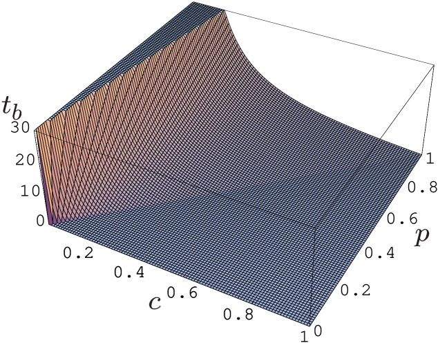
Figure 1: The time for which the coherence of a qubit can be kept constant, as a function of coherence $c$ and purity $p$, for $\gamma=0.1$.

In Fig. 1 we plot the breakdown time $t_{b}$ as a function of coherence $c$ and purity $p$, for $\gamma=0.1$. The plot reflects the constraint $c\leq p$, and shows the tradeoff between coherence and the time for which it can be maintained.

It is interesting to compare the controlled and uncontrolled dynamics. We again set $\gamma=0.1$, and in the controlled scenario choose an initial state which lies in a region of Fig. 1 where there is some coherence to be preserved: $c=0.3$ and $p=0.8$. This implies $v_{z}(0)=\sqrt{p(0)-c}=1/\sqrt{2}$. We set $v_{x}(0)=v_{y}(0)$, so that $v_{x}(0)=\sqrt{c/2}=\sqrt{0.3/2}\approx 0.39$. A comparison of the two cases is plotted in Fig. 2. In the uncontrolled scenario of pure dephasing $v_{z}$ is a constant of motion, while $v_{x}$ decays monotonically. In contrast, in the controlled case these roles are reversed in spite of the dephasing: the control fixes $v_{x}$ while $v_{z}$ is allowed to decay.

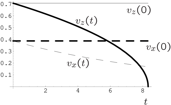
Figure 2: Comparison between the controlled (thick lines) and the free (thin lines) evolution for $v_{z}$ and $v_{x}$. Here $\gamma=0.1$, $c=0.3$, $p=0.8$, $v_{x}(0)=v_{y}(0)$.

The control fields necessary to keep the coherence constant are plotted in Fig. (3), where we have chosen $\omega_{0}(t)\equiv\omega_{0}$ to account for an energy difference between the two qubit states. For the plot we set $\omega_{0}=4.0$. All other parameters and the initial state are as in Fig. (2). The divergence of the control fields at $t_{b}$ is clearly visible.

Figure 3: Control fields $\omega_{1}$ (solid line) and $\omega_{2}(t)$ (dashed line). Parameters as in Fig. (2), and $\omega_{0}=4.0$.

Geometrically, the uncontrolled phase-flip channel maps the the Bloch sphere to an ellipsoid with the $z$-axis as major axis and minor axis in the $x-y$ plane. As is clear from Eqs. (46), the major axis is invariant under the uncontrolled dynamics, while the minor axis (the coherence) is contracted. On the other hand, in the controlled scenario, the minor axis is invariant up until the breakdown time ($c$ is constant), while the major axis is contracted [Eq. (52)]. The control field is thus able to trade the contraction in the $x-y$ plane for one along the $z$-axis. The geometric interpretation of this process is the following: the control field attempts to rotate the ellipsoid so that the minor axis becomes as aligned as possible with the $z$-axis, where it would experience no contraction. The rotation takes the minor axis to an invariant point, which requires ever-growing control field amplitude, until the contraction is so strong that the control field is no longer capable of sustaining the required rotation, and diverges. The effectiveness of this process depends on the desired value of coherence that is to be maintained, and the initial purity. This rotational interpretation follows from Eq. (42): we have, in the simplest case of constant $\omega_{0}(t)$, $\vec{\Omega}(t)=(\omega_{1}(t),-\omega_{2}(t),\omega_{0})$ [a force vector whose length in the $x-y$ plane is growing monotonically for $0\leq t\leq t_{b}$ ($|\vec{\Omega}(t)|^{2}=\frac{(\gamma^{2}+\omega_{0}^{2})c}{v_{z}^{2}(0)-2\gamma ct}+\omega_{0}^{2}$)], multiplying via the vector cross-product the vector $\vec{v}(t)=(v_{x}(0),v_{y}(0),\sqrt{v_{z}^{2}(0)-2\gamma ct})$ [a vector with fixed coordinates in the $x-y$ plane whose magnitude is shrinking monotonically], thus producing a rate of change of $\vec{v}(t)$ pointing in the plane orthogonal to $\vec{\Omega}(t)$ and $\vec{v}(t)$.

IV Decoherence equivalence classes

From the geometric interpretation given above it is clear that there are other decoherence models where the Bloch sphere experiences a similar deformation, but the contraction happens in a different plane. Then the question arises which decoherence models are “equivalent” in the sense that what we have learned from the above phase flip channel can be applied directly to another decoherence model.

Suppose we apply a global unitary transformation $U$ to each Lindblad operator in the master equation (1), as well as to the control Hamiltonian $H$. We will say that two decoherence problems which are thus related are in the same unitary equivalence class. Under this transformation the master equation becomes

$$\frac{\partial\rho}{\partial t}=-\frac{i}{\hbar}[UHU^{\dagger},\rho]+\frac{1}{2}\sum_{i,j}a_{ij}\left([UF_{i}U^{\dagger}\rho,UF_{j}^{\dagger}U^{\dagger}]+[UF_{i}U^{\dagger},\rho UF_{j}^{\dagger}U^{\dagger}]\right).$$ (58)

This is the “Heisenberg picture”. We can transform to the “Schrodinger picture” by multiplying the latter master equation by $U$ from the right and $U^{\dagger}$ from the left:

$$\frac{\partial\rho^{\prime}}{\partial t}=-\frac{i}{\hbar}[H,\rho^{\prime}]+\frac{1}{2}\sum_{ij}a_{ij}\left([F_{i}\rho^{\prime},F_{j}]+[F_{i},\rho^{\prime}F_{j}]\right),$$ (59)

where $\rho^{\prime}=U^{\dagger}\rho U$. This is the same as the original master equation, but for a transformed $\rho$. E.g., the phase flip channel ($\sigma_{z}$-decoherence) is unitarily related to the bit flip channel ($\sigma_{x}$-decoherence) via the Hadamard matrix $U=\frac{1}{\sqrt{2}}\left(\begin{array}[]{cc}1&1\\ 1&-1\end{array}\right)$.

In the coherence vector representation the unitary transformation $U$ becomes a real rotation matrix $R$ of the coherence vector via the appropriate adjoint representation Cornwell:84II ; e.g., for the qubit problem $U\in\mathrm{SU}(2)$ while $R\in\mathrm{SO}(3)$. The analog of Eq. (59) [i.e., the transformed Eq. (20)] is

$$\dot{\vec{v}}^{\prime}=(M_{0}+M(t))\vec{v}^{\prime}+\vec{k}$$ (60)

where $M_{0}$ and $\vec{k}$ are the effects of decoherence in the coherence vector representation Alicki:87 , $\vec{v}^{\prime}=R\vec{v}$, and $M(t)$ represents the Hamiltonian control [recall Eq. (30)].

Thus, two decoherence problems which are in the same unitary equivalence class differ, in the “Schrodinger picture”, by a fixed rotation of the coherence vector $\vec{v}$. In terms of the control problem at hand, the stabilization of the coherence $c$, it is then clear that the control solution for all decoherence problems which are in the unitary equivalence class of pure dephasing is still given by the result derived above, i.e., by Eqs. (56),(57). The difference between the decoherence problems in this equivalence class lies only in the initial values of $v_{x}(0)$, $v_{y}(0)$ and $v_{x}(0)$, which enter into the explicit form of the control fields through the expressions (56),(57). As a very simple example, consider the case of transforming from the phase-flip channel to the unitarily equivalent $-$(phase-flip channel), i.e., $\sigma_{z}\mapsto-\sigma_{z}$. There should, on physical grounds, be no essential difference between these two cases. Indeed, in this case $U=\exp(i\pi\sigma_{y}/2)$, and the adjoint $\mathrm{SO}(3)$ matrix is a rotation by $\pi$ about the $y$-axis, i.e., $R=\mathrm{diag}\left(-1,1,-1\right)$. Thus $\vec{v}^{\prime}=R\vec{v}=(-v_{x},v_{y},-v_{z})$, and both the coherence $c=v_{x}^{2}+v_{y}^{2}$ and $v_{z}^{2}$ are invariant, so that the transformed control fields [compare to Eqs. (56),(57)], given in terms of the untransformed coherence vector,

$$\omega_{2}^{\prime}(t) = \left(\pm\right)\frac{+\gamma v_{x}(0)-\omega_{0}(t)v_{y}(0)}{\sqrt{v_{z}^{2}(0)-2\gamma ct}},$$ (61)

$$\omega_{1}^{\prime}(t) = \left(\pm\right)\frac{-\gamma v_{y}(0)-\omega_{0}(t)v_{x}(0)}{\sqrt{v_{z}^{2}(0)-2\gamma ct}},$$ (62)

have exactly the same divergence as before. The fact that there is a difference at all, is a reflection of the fact that the mapping from $\mathrm{SU}(2)$ to $\mathrm{SO}(3)$ is homomorphic (double-valued) Cornwell:84II ; indeed, the master equation (44) is invariant under the transformation $\sigma_{z}\mapsto-\sigma_{z}$, but this is not the case in the coherence vector representation [the corresponding $M_{0}$ in Eq. (60) is not invariant].

It is worth emphasizing that the equivalence class of pure dephasing is the entire group $\mathrm{SU}(2)$, but it excludes important processes such as spontaneous emission (represented by $\sigma_{-}\notin\mathrm{SU}(2)$]. More generally, linear combinations of Pauli matrices, corresponding to affine shifts in the coherence vector representation, are not in the equivalence class of pure dephasing. The solution of the control problem for such processes is deferred to a future publication; it involves solving the non-linear tracking equation (35) for these cases.

V Singularities

It is insightful to reformulate the above control problem in terms of the tracking control framework of Ref. Zhu:99 , which allows one to study the nature of the control field singularity. We once again linearize the quadratic control objective $c(t)=c(0)$ into a two-dimensional form where we wish to separately control $v_{x}(t)$ and $v_{y}(t)$ (in particular, keep them constant), using the two control fields $\omega_{1}(t)$ and $\omega_{2}(t)$. Following the notation of Ref. Zhu:99 as closely as possible we have [recall Eqs. (20),(30)]

$$\dot{\vec{v}}=(M_{0}+\sum_{j=0}^{2}\omega_{j}(t)\Lambda_{j})\vec{v}+\vec{k},$$ (63)

and the control objectives $S_{1}=v_{x}$ and $S_{2}=v_{y}$ are

$$S_{i}(t)=\vec{v}^{t}(t)\cdot O_{i}\cdot\vec{v}(t)~{}~{}[=S_{i}(0)],$$ (64)

with

$$O_{1}=\left(\begin{array}[]{ccc}1&0&0\\ 0&0&0\\ 0&0&0\end{array}\right),\quad O_{2}=\left(\begin{array}[]{ccc}0&0&0\\ 0&1&0\\ 0&0&0\end{array}\right).$$ (65)

The matrices $\Lambda_{j}$, defined in Eq. (31), satisfy

$$[O_{1},\Lambda_{1}]=[O_{2},\Lambda_{2}]=0.$$ (66)

Using this fact, Eq. (63), and the observation $\Lambda_{j}^{t}=-\Lambda_{j}$, it is simple to show by explicit differentiation of Eq. (64) that

$$\omega_{1}(t) = \frac{\dot{S}_{2}+\omega_{0}(t)\vec{v}^{t}[\Lambda_{0},O_{2}]\vec{v}-\vec{v}^{t}\{M_{0},O_{2}\}\vec{v}-\vec{k}^{t}O_{2}\vec{v}-\vec{v}^{t}O_{2}\vec{k}}{\vec{v}^{t}[\Lambda_{1},O_{2}]\vec{v}},$$ (67)

$$\omega_{2}(t) = \frac{\dot{S}_{1}+\omega_{0}(t)\vec{v}^{t}[\Lambda_{0},O_{1}]\vec{v}-\vec{v}^{t}\{M_{0},O_{1}\}\vec{v}-\vec{k}^{t}O_{1}\vec{v}-\vec{v}^{t}O_{1}\vec{k}}{\vec{v}^{t}[\Lambda_{2},O_{1}]\vec{v}},$$ (68)

where $\{,\}$ denotes the anti-commutator and its appearance in the expression involving the decoherence matrix $M_{0}$, rather than a commutator, is a manifestation of the associated damping. These equations are equivalent to Eqs. (33),(34), and can be further simplified by using the constraint of constant coherence ($\dot{S}_{1,2}=0$), and the explicit forms of the various vectors and matrices appearing in them.

Clearly, a singularity arises when the denominators in Eqs. (67),(68) vanish:

$$\vec{v}^{t}(t)[\Lambda_{1},O_{2}]\vec{v}(t) = 0,$$ (69)

$$\vec{v}^{t}(t)[\Lambda_{2},O_{1}]\vec{v}(t) = 0.$$ (70)

Ref. Zhu:99 distinguishes between several types of singularities: (i) A trivial singularity is the case when the denominators are zero over a continuous time domain, (ii) A non-trivial singularity is the case when the denominators are zero at isolated points. A trivial singularity can be removed by taking higher order time-derivatives of Eq. (64) under the conditions (69),(70), until the trivial singularity is removed (i.e., a non-zero denominator is found). If derivatives of all orders result in a trivial singularity, the system is uncontrollable.

In our case, using

$$[\Lambda_{1},O_{2}]=\left(\begin{array}[]{ccc}0&0&0\\ 0&0&1\\ 0&1&0\end{array}\right),\quad[\Lambda_{2},O_{1}]=\left(\begin{array}[]{ccc}0&0&1\\ 0&0&0\\ 1&0&0\end{array}\right),$$ (71)

we have

$$\vec{v}^{t}(t)[\Lambda_{1},O_{2}]\vec{v}(t) = 2v_{y}(t)v_{z}(t),$$ (72)

$$\vec{v}^{t}(t)[\Lambda_{2},O_{1}]\vec{v}(t) = 2v_{x}(t)v_{z}(t).$$ (73)

Since our control fields keep $v_{x,y}$ fixed, the singularity arises at the isolated point $v_{z}(t_{b})=0$. We are thus dealing with a non-trivial singularity. There are now two subcases: a) The singularity is of the form $\omega_{j}(t)=\alpha/0$ with $\alpha\neq 0$; b) The singularity is of the form $\omega_{j}(t)=0/0$. In case b) one can apply L’Hospital’s rule and (sometimes) overcome the singularity. In our case, the numerators in Eqs. (67),(68) involve the decoherence matrix $M_{0}$ (and the affine shift $\vec{k}$), while the denominators involve only the controls, so that generically one cannot expect a cancellation as in case b). Ref. Zhu:99 concludes that in case a) there is no solution for the field and the system is uncontrollable at the singular point. This conclusion agrees with our geometric interpretation of Sec. III.3.

VI Conclusions and Open Questions

In this work we have considered the problem of controlling the coherence of a single qubit under circumstances where none of the encoding or dynamical decoupling methods recently developed in quantum information science apply. Instead we have employed a version of tracking control, where a control field is continuously adjusted in order to satisfy the objective of constant coherence. This is possible up to a finite time, which depends on the initial coherence, at which the control field diverges.

There are various open questions suggested by these results.

i) While our original goal was to track the coherence $c=v_{x}^{2}+v_{y}^{2}$, we in fact solved the more restrictive problem of separately controlling $v_{x}$ and $v_{y}$. It would be interesting to consider the case where these components are allowed to vary while truly trying to fix only $c$. In particular, it would be interesting to see if this enables the extension of the breakdown time.

ii) Expansion of the Hilbert space by including additional levels: Controllability could improve if instead of having a two-level system we were to use an $n$-level system, where we coherently control all the $n$ levels, but use just two for the qubit. Within this larger Hilbert space it is possible that interference effects could be used profitably to maintain the coherence of the two qubit levels, as e.g., in electromagnetically induced transparency Harris:97 , or control of vibrational wavepackets Brif:01 .

iii) Periodic or continuous update of the control objective so as to reduce the desired value of coherence: In this manner the singularity of the control fields can be avoided for arbitrarily long times. It would be interesting to formulate this as an optimal control problem, with the objective being, e.g., the time-integral of coherence.

iv) As discussed above, the control fields depend crucially on the knowledge of the initial state whose coherence we wish to maintain. For certain states [with $v_{z}(0)=0$] no such control is possible. Additionally we need to know $v_{x}(0)$ and $v_{y}(0)$ in order to correctly apply the control fields. The full tracking control problem requires knowing even more: the full coherence vector $\vec{v}(t)$, an impossible task due to the non-commutativity of the observables involved. In general, one can envision performing quantum tracking control based on the incomplete information gleaned in real time from measuring an as large as possible set of commuting observables. It is an open problem to estimate the quality of the (partial) tracking one can thus attain.

v) As mentioned in Sec. II.1, the purity for non-unital decoherence channels can actually increase without control. Unitary, open-loop control in this case was studied in Ref. Recht:02 , It would be interesting to explore coherence tracking control for this class of channels.

vi) Finally, an important extension of the results reported here would be to problems involving more than one qubit, e.g., in order to preserve entanglement.

- (1) M.A. Nielsen and I.L. Chuang, Quantum Computation and Quantum Information (Cambridge University Press, Cambridge, UK, 2000).
- (2) P.W. Brumer and M. Shapiro, Principles of the Quantum Control of Molecular Processes (Wiley, 2003).
- (3) For a review see A.M. Steane, in Introduction to Quantum Computation and Information, edited by H.K. Lo, S. Popescu and T.P. Spiller (World Scientific, Singapore, 1999), pp. 184–212.
- (4) For a review see D.A. Lidar, K.B. Whaley, in Irreversible Quantum Dynamics, Vol. 622 of Lecture Notes in Physics, edited by F. Benatti and R. Floreanini (Springer, Berlin, 2003), p. 83, eprint quant-ph/0301032.
- (5) For an overview see L. Viola, Phys. Rev. A 66, 012307 (2002).
- (6) For an overview see M.S. Byrd, L.-A. Wu, D.A. Lidar, J. Mod. Optics, in press (2004), eprint quant-ph/0402098.
- (7) P. Facchi, D.A. Lidar, and S. Pascazio, Phys. Rev. A 69, 032314 (2004).
- (8) R.M. Hirschorn, SIAM J. Control Optim. 17, 289 (1979).
- (9) R.M. Hirschorn, IEEE Trans. Autom. Control. 26, 593 (1981).
- (10) R.M. Hirschorn and J. Davis, SIAM J. Control Optim. 26, 1321 (1988).
- (11) Z. Retchkiman, J. Alvarez, and R. Castro, Int. J. Robust Nonlin. Control 5, 553 (1995).
- (12) B. Jakubczyk and F. Lamnabhi-Lagarrigue, Int. J. Robust Nonlin. Control 21, 271 (1993).
- (13) Y. Chen, P. Gross, V. Ramakrishna, H. Rabitz, and K. Mease, J. Chem. Phys. 102, 8001 (1995).
- (14) Z.-M. Lu and H. Rabitz, J. Phys. C 99, 13731 (1995).
- (15) P. Gross, H. Singh, H. Rabitz, K. Mease, and G. Huang, Phys. Rev. A 47, 4593 (1993).
- (16) W. Zhu, M. Smit, and H. Rabitz, J. Chem. Phys. 110, 1905 (1999).
- (17) W. Zhu, J. Botina, and H. Rabitz, J. Chem. Phys. 108, 1953 (1998).
- (18) W. Zhu and H. Rabitz, J. Chem. Phys. 119, 3619 (2003).
- (19) L. Bouten, S. Edwards, and V.P. Belavkin, eprint quant-ph/0407192.
- (20) V.P. Belavkin, Radiotechnika i Electronika 25, 1445 (1980).
- (21) B. Recht, Y. Maguire, S. Lloyd, I.L. Chuang, N.A. Gershenfeld, eprint quant-ph/0210078.
- (22) R. Alicki and K. Lendi, Quantum Dynamical Semigroups and Applications, No. 286 in Lecture Notes in Physics (Springer-Verlag, Berlin, 1987).
- (23) C. Altafini, J. Math. Phys. 44, 2357 (2003).
- (24) C. Altafini, Phys. Rev. A, in press (2004).
- (25) W. Ketterle and D.E. Pritchard, Phys. Rev. A 46, 4051 (1992).
- (26) D.J. Tannor and A. Bartana, J. of Phys. Chem. A 103, 10359 (1999).
- (27) R. Bhatia, Matrix Analysis, No. 169 in Graduate Texts in Mathematics (Springer-Verlag, New York, 1997).
- (28) J.F. Cornwell, Group Theory in Physics, Vol. II of Techniques of Physics: 7 (Academic Press, London, 1984).
- (29) D.A. Steck, K. Jacobs, H. Mabuchi, T. Bhattacharya, S. Habib, Phys. Rev. Lett. 92, 223004 (2004).
- (30) S.E. Harris, Physics Today 50, 36 (1997).
- (31) C. Brif, H. Rabitz, S. Wallentowitz, and I.A. Walmsley, Phys. Rev. A 63, 063404 (2001).