Bound and resonance states of the nonlinear Schrödinger equation in simple model systems

Abstract

The stationary nonlinear Schrödinger equation, or Gross–Pitaevskii equation, is studied for the cases of a single delta potential and a delta–shell potential. These model systems allow analytical solutions, and thus provide useful insight into the features of stationary bound, scattering and resonance states of the nonlinear Schrödinger equation. For the single delta potential, the influence of the potential strength and the nonlinearity is studied as well as the transition from bound to scattering states. Furthermore, the properties of resonance states for a repulsive delta–shell potential are discussed.

1 Introduction

In the case of low temperatures, the dynamics of a Bose–Einstein condensate can be described in a mean–field approach by the nonlinear Schrödinger equation or Gross–Pitaevskii equation [1]. We will focus on the one–dimensional case, which can be achieved experimentally by a tight confinement in the two other spatial directions (see for example [2] and references therein). The nonlinear Schrödinger equation for the macroscopic wavefunction is then given by

$$\left(-\frac{\hbar^{2}}{2m}\frac{\partial^{2}}{\partial x^{2}}+V(x)+g|\psi(x,t)|^{2}\right)\psi(x,t)={\rm i}\hbar\,\frac{\partial\psi(x,t)}{\partial t},$$ (1)

where $g=4\pi\hbar^{2}aN/m$ is the nonlinear “interaction strength” and $N$ is the number of particles in the condensate. The wavefunction is normalized to $\|\psi\|=1$. In this ansatz, one only takes elastic $s$–wave scattering into account, characterized by the $s$–wave scattering length $a$. The scattering length $a$ and thus the nonlinearity $g$ are negative for an attractive nonlinear interaction and positive for a repulsive one. Another important application of the nonlinear Schrödinger equation is the propagation of electromagnetic waves in nonlinear media (see, e.g., [3], Ch. 8).

Analytic solutions of the nonlinear equation for a non–vanishing potential $V(x)$ are rare and therefore it is of interest to study such a simple case in some detail. Here we study the nonlinear Schrödinger equation for two simple potentials: a single delta potential

$$V(x)=\lambda\delta(x),$$ (2)

modelling a short range interaction, and the delta–shell potential

$$V(x)=\left\{\begin{array}[]{*{2}{l}}+\infty&\mbox{for}\,x<0\\ \lambda\delta(x-a)&\mbox{for}\,x\geq 0\\ \end{array}\right.$$ (3)

with $a>0$. The delta–shell is a popular model system for the study of resonances and decay. We confine ourselves to the stationary case, where the time dependence is given by the factor ${\rm e}^{-{\rm i}\mu t/\hbar}$. Using units with $\hbar=1$ and $m=1$, the stationary nonlinear Schrödinger equation reads

$$\left(-\frac{1}{2}\frac{{\rm d}^{2}}{{\rm d}x^{2}}+V(x)+g|\psi(x)|^{2}\right)\psi(x)=\mu\,\psi(x).$$ (4)

The solutions of equation (4) for the delta potential and the delta–shell potential are essentially the ones of the free nonlinear Schrödinger equation. The wavefunction itself is continuous, but due to the delta potential, its first derivative is discontinuous at $x=0$, resp. $x=a$:

$$\lim_{\epsilon\to 0+}\big{(}\psi^{\prime}(a+\epsilon)-\psi^{\prime}(a-\epsilon)\big{)}=2\lambda\psi(a).$$ (5)

One can easily show that this behaviour, well–known for the Schrödinger equation, is not changed by the nonlinearity. Furthermore, in the case of the delta–shell potential, the boundary condition $\psi(0)=0$ has to be obeyed.

2 Single delta potential

The single delta potential (2) is the easiest model for the study of the existence and the properties of bound and scattering states. It has been studied in the context of a nonlinear flow [4, 5], however rather briefly.

In the linear case, $g=0$, equation (4) with $\lambda<0$ supports a single bound state with energy $E_{0}=-\lambda^{2}/2$ and a continuous spectrum for $E>0$, however, without embedded resonances. The normalized bound state wavefunction is

$$\psi_{0}(x)=\sqrt{|\lambda|}\,{\rm e}^{\,\lambda|x|}\,.$$ (6)

In the following, we will study the modifications of this linear case due to an attractive resp. repulsive nonlinearity. By means of the scaling $x=x^{\prime}/|g|$, $\psi=\psi^{\prime}\sqrt{|g|}$, $\lambda=\lambda^{\prime}|g|$ and $\mu=\mu^{\prime}g^{2}$ (which conserves the normalization), the parameter $g$ in (4) can be removed up to a sign. Therefore we will fix the nonlinearity to $g=\pm 1$ (with the exception of section 2.3).

2.1 Attractive nonlinearity

In the case of an attractive nonlinearity, $g=-1$, the nonlinear Schrödinger equation (4) has the well–known bright soliton solution for $\lambda=0$ and $\mu<0$ [6, 7],

$$\psi(x)=k\,{\rm sech}\big{(}k\,(x-x_{0})\big{)}\quad\mbox{with}\quad k=\sqrt{-2\mu}\,.$$ (7)

In order to find nonlinear bound states, i.e. normalizable solutions of equation (4), bright soliton solutions of the form (7) for $x>0$ and $x<0$ are matched at $x=0$ by means of condition (5). Obviously, the wavefunction $\psi(x)$ has to be symmetric with respect to $x=0$ and is therefore given by expression (7) for $x\geq 0$ and $\psi(x)=\psi(-x)$ otherwise. Inserting this ansatz into equation (5) leads to the condition

$$\tanh(kx_{0})=\lambda/k\,.$$ (8)

Combined with the normalization of the wavefunction,

$$1 = \int_{-\infty}^{+\infty}\big{|}\psi(x)\big{|}^{2}\,{\rm d}x=2k^{2}\int_{0}^{+\infty}{\rm sech}^{2}\big{(}k\,(x-x_{0})\big{)}\,{\rm d}x$$ (9)

$$= 2k\big{(}1+\tanh(kx_{0})\big{)}\,,$$

this yields

$$k={\textstyle\frac{1}{2}}-\lambda\ ,\quad\mbox{i.e.}\quad\mu=-{\textstyle\frac{1}{8}}(2\lambda-1)^{2}\,.$$ (10)

Because of $|\tanh(kx_{0})|<1$, one finds a condition for the existence of a bound state:

$$\lambda<\lambda_{c}={\textstyle\frac{1}{4}}\,.$$ (11)

A bound state exists for any attractive delta potential but also for a repulsive one, provided that its strength is not too large. This effect is due to the attractive self interaction $-|\psi(x)|^{2}$ which can compensate a limited external repulsion.

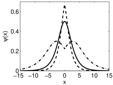
Figure 1: Wavefunctions $\psi(x)$ of bound states of the nonlinear Schrödinger equation (attractive nonlinearity, $g=-1$) for a delta potential $V(x)=\lambda\delta(x)$ with $\lambda=-0.2$ ($---$), $\lambda=0$ (—) and $\lambda=+0.2$ ($-\cdot-$).

Figure 1 shows the wavefunctions for such bound states for three different values of the potential strength $\lambda$. Quite generally, for an attractive delta potential with a negative value of $x_{0}$, the wavefunction tends to concentrate at the delta potential with decreasing $\lambda$. A repulsive delta potential repels the wavefunction, $x_{0}$ is positive, and one observes two peaks of $\psi(x)$ at $x=\pm x_{0}$ that are pushed further away as $\lambda$ is increased toward $\lambda_{c}$. For $\lambda\rightarrow\lambda_{c}$ the wavefunction evolves into two infinitely separated bright soliton solutions.

Remarkably, the bound state ceases to exist at a finite negative value of the chemical potential

$$\mu_{c}=-{\textstyle\frac{1}{8}}(2\lambda_{c}-1)^{2}=-{\textstyle\frac{1}{32}}\,.$$ (12)

This difference to the linear equation or the case of repulsive nonlinearity (see below) corresponds to the fact that the wavefunction is no longer bound by an external potential but by the internal self–interaction.

For $\lambda>\lambda_{c}$, there is no bound state solution any more, but one can actually find periodic stationary solutions in terms of Jacobi elliptic functions [6, 7]

$$\psi(x)=\frac{\sqrt{p},4K(p)}{L}\,{\rm cn}\bigg{(}4K(p)\frac{x-x_{0}}{L}\,\bigg{|}\,p\bigg{)}.$$ (13)

Here $L$ is the period, $p\in[0,1]$ the elliptic modulus of the Jacobi elliptic function ${\rm cn}$ and $K(p)$ denotes the complete elliptic integral of the first kind. The chemical potential is related to these parameters by

$$\mu=8(1-2p)\,K^{2}(p)/L^{2}\,.$$ (14)

These solutions are of course no longer normalizable, and will be denoted as scattering states in the following. Such a periodic solution, characterized by three parameters, the chemical potential $\mu$, the period $L$ and the shift $x_{0}$, has to fulfil only condition (5). Thus, for a fixed value of the potential strength $\lambda$, there exists a variety of solutions, whereby the chemical potential $\mu$ and the period $L$ can be chosen more or less independently. The value of $x_{0}$ is then fixed to satisfy condition (5).

In the following, we discuss a particular class of solutions that merge continuously into the bound state solution when $\lambda$ is decreased below its critical value $\lambda_{c}$. Therefore we make the ansatz that $\mu$ and $\psi(x=0)$ depend continuously on the strength $\lambda$ of the delta potential at $\lambda_{c}$. In fact, we assume the functional relation to be the same for $\lambda>\lambda_{c}$ and $\lambda<\lambda_{c}$, i.e. given by equation (10), and

$$\psi(0)=k\,{\rm sech}\left({\rm arctanh}(\lambda/k)\right),$$ (15)

respectively. For a given value of $\lambda$, we construct solutions (13) that fulfil condition (5) and yield the desired values of $\mu$ and $\psi(0)$. Such solutions can indeed be found and figure 2 illustrates such a wavefunction for $\lambda=0.26$, just above the critical value $\lambda_{c}=0.25$, in comparison to a bound state solution for $\lambda=0.24$.

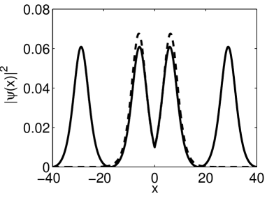
Figure 2: Wavefunctions of a bound state ($--$, $\lambda=0.24$) and a scattering state (—, $\lambda=0.26$) for a repulsive delta potential $V(x)=\lambda\delta(x)$ for an attractive nonlinearity close to the transition at $\lambda_{c}=0.25$.

In the vicinity of the delta potential at $x=0$, both wavefunctions look rather similar and thus the transition from a bound to a scattering state seems to be continuous. The observed difference between the bound state and the periodic solution for $|x|>L$ disappears in the limit $\lambda\searrow\lambda_{c}$ because the period $L$ of the Jacobi elliptic solution moves toward infinity.

To explore this transition in some detail, we consider the position $x_{0}$ of the first maximum of $|\psi(x)|^{2}$, as a function of $\lambda$, given by

$$x_{0}(\lambda)=\frac{1}{1/2-\lambda}\,{\rm arctanh}\left(\frac{\lambda}{1/2-\lambda}\right)$$ (16)

for $\lambda<\lambda_{c}$ and by the solution of the complex equations

$$\psi(0) = k\sqrt{\frac{p}{2p-1}}\;{\rm cn}\bigg{(}\frac{kx_{0}(\lambda)}{\sqrt{2p-1}}\,\bigg{|}\,p\bigg{)}\quad{\rm and}$$

$$\lambda\psi(0) = k^{2}\frac{\sqrt{p}}{2p-1}\;{\rm sn}\bigg{(}\frac{kx_{0}(\lambda)}{\sqrt{2p-1}}\,\bigg{|}\,p\bigg{)}\;{\rm dn}\bigg{(}\frac{kx_{0}(\lambda)}{\sqrt{2p-1}}\,\bigg{|}\,p\bigg{)}$$ (17)

for $\lambda>\lambda_{c}$, where $k$ and $\psi(0)$ are fixed by equations (10) and (15) as discussed above. At $\lambda_{c}$, the function $x_{0}(\lambda)$ shown in figure 3 on the left has a logarithmic singularity.

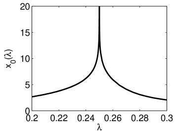
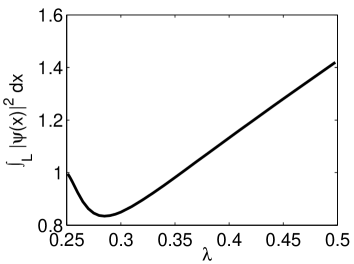
Figure 3: Transition from a bound to a scattering state. Left: Position $x_{0}(\lambda)$ of the first maximum of the wavefunction. Right: Norm per period $L$. Note that $L\to\infty$ as $\lambda\searrow\lambda_{c}$.

On the right of figure 3, the norm per period $\int_{-L/2}^{L/2}|\psi(x)|^{2}{\rm d}x$ is displayed, which tends to unity at the critical point $\lambda_{c}$, i.e. it approaches the bound state normalization. Hence the norm is also continuous.

2.2 Repulsive nonlinearity

In the case of a repulsive nonlinearity, $g=+1$, the nonlinear Schrödinger equation has the well–known dark soliton solutions for $\lambda=0$ [8, 7]:

$$\psi=\sqrt{\mu}\,\tanh{\left(\sqrt{\mu}(x-x_{0})\right)}.$$ (18)

Making such an ansatz separately for $x>0$ and $x<0$ and matching at $x=0$ with respect to condition (5) yields $x_{0}=0$ regardless of the value of $\lambda$. Remarkably, the wavefunction has a zero at $x=0$ even for an attractive delta potential. But solutions of this kind are of course not normalizable. Another possible solution is

$$\psi(x)=k\,{\rm cosech}(k\,(x-x_{0}))\ ,\quad\mbox{with}\quad k=\sqrt{-2\mu}\,,$$ (19)

which is usually discarded because of its unphysical singularity at $x=x_{0}$. In the case of a delta potential, however, this ansatz reveals proper stationary bound states. Assuming (19) for $x>0$, a short calculation shows that the wavefunction has to be symmetric, $\psi(-x)=\psi(x)$. In addition, $x_{0}$ must be negative because otherwise the wavefunction would become singular at $x=x_{0}$. Condition (5) yields

$$\tanh(kx_{0})=k/\lambda$$ (20)

and the normalization of the wavefunction requires

$$1 = \int_{-\infty}^{+\infty}\big{|}\psi(x)\big{|}^{2}\,{\rm d}x=2k^{2}\int_{0}^{+\infty}\!\!{\rm cosech}^{2}\big{(}k\,(x-x_{0})\big{)}\,{\rm d}x$$ (21)

$$= -2k\big{(}1+\coth(kx_{0})\big{)}\,.$$

This leads to

$$k=-{\textstyle\frac{1}{2}}-\lambda$$ (22)

which must be positive, yielding the condition

$$\lambda<\lambda_{c}=-{\textstyle\frac{1}{2}}\,,$$ (23)

i.e. the delta potential must be sufficiently attractive to overcome the repulsive self–interaction in order to support a bound state.

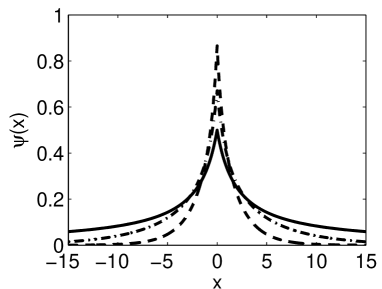
Figure 4: Wavefunctions $\psi(x)$ of bound states of the nonlinear Schrödinger equation (repulsive nonlinearity, $g=+1$) for a delta potential $V(x)=\lambda\delta(x)$ for three values of the potential strength $\lambda=-1$ ($---$), $\lambda=-0.7$ ($-\cdot-$) and for the critical case $\lambda=-0.5$ (—) .

In figure 4, such bound states are displayed for different values of the potential strength $\lambda$. For decreasing values of $\lambda$, the wavefunction concentrates at the position of the delta potential. In the opposite limit, $\lambda\nearrow\lambda_{c}$, we see by series expansion of the $\tanh$ and the $\sinh$ functions, that

$$x_{0}\to x_{c}=1/\lambda_{c}\quad\mbox{and}\quad\mu\to\mu_{c}=0$$ (24)

and that the wavefunction converges to the limiting function

$$\psi_{c}(x)=\frac{1}{|x|-x_{c}}=\frac{1}{|x|+2}$$ (25)

also shown in figure 4. This is in contrast to the case of an attractive nonlinearity where the bright soliton peaks move to $\pm\infty$ at the critical value $\lambda_{c}$.

For $\lambda>\lambda_{c}$, one again finds periodic solutions in terms of Jacobi elliptic functions [8, 7]

$$\psi(x)=\frac{\sqrt{p}\,4K(p)}{L}\,{\rm sn}\bigg{(}4K(p)\frac{x-x_{0}}{L}\,\bigg{|}\,p\bigg{)},$$ (26)

where $L$ is the periodicity, $p\in[0,1]$ the elliptic modulus of the Jacobi elliptic function and $K(p)$ denotes the complete elliptic integral of the first kind. The chemical potential is given by

$$\mu=8(p+1)\,K(p)^{2}/L^{2}.$$ (27)

For a fixed value of the potential strength $\lambda$, one again finds a variety of solutions, whereby the chemical potential $\mu$ and the period $L$ can be chosen more or less independently. Note that such periodic solutions can only be found for $\mu>0$.

Nevertheless, one can find a lower bound for the period $L$. From equation (27) it follows that

$$L=\sqrt{\frac{8(p+1)}{\mu}}\,K(p)\geq\frac{2\pi}{\sqrt{2\mu}}\,.$$ (28)

For $\lambda\searrow\lambda_{c}$ and $\mu\searrow 0$ the period of the wavefunction $L$ tends to infinity and the wavefunction is not periodic any more in this limit. But in this case one cannot find a continuous transition to the bound state wavefunction (19). For $\lambda\nearrow\lambda_{c}$ one finds the bound state (25) with $\psi(0)=1/2$ and $\mu=0$. In contrast, we have $\psi(0)\rightarrow 0$ for $\mu\searrow 0$ for the periodic solution (26) because of equation (27). In fact, the elliptic function ${\rm sn}$ evolves continuously into the $\tanh$ when the elliptic modulus $p$ tends to unity [9].

Actually, there exist Jacobi elliptic functions that merge continuously into the cosech as the elliptic modulus $p$ tends to one. These solutions are given in terms of the Jacobi elliptic functions ds and cs [9]. But these functions have poles at the zeros of the ${\rm sn}$ and thus are not physical.

2.3 Variation of the nonlinearity

In this section, we will briefly discuss the influence of the mean–field interaction strength, i.e. the nonlinearity $g$, on the solutions of the nonlinear Schrödinger equation for an attractive delta potential. We therefore reintroduce the parameter $g$.

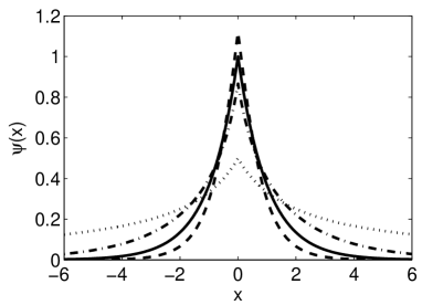
Figure 5: Bound state wavefunctions $\psi(x)$ of the nonlinear Schrödinger equation for an attractive delta potential $V(x)=-\delta(x)$ for different values of the nonlinearity: $g=-1$ ($--$), $g=0$ (—), $g=+1$ ($-\cdot-$) and $g=g_{c}=2$ ($\cdot\cdot\cdot$) .

The bound state solutions have already been deduced in the previous sections. In figure 5, the wavefunction of such a bound state is displayed for three different values of the nonlinearity $g=-1,\,0,\,+1$ and a fixed potential strength $\lambda=-1$. With increasing nonlinearity $g$, the wavefunction is pushed outward.

In both cases of attractive and repulsive nonlinearity, the chemical potential is given by

$$\mu=-\frac{1}{8}\left(2\lambda+g\right)^{2}\,,$$ (29)

which follows directly from the matching condition (5) and the normalization of the wavefunction. At a critical value of $g$, the chemical potential $\mu$ becomes zero and the bound state ceases to exist. The condition for the existence of a bound state is the same as discussed in section 2.2. Reformulated in terms of the nonlinearity parameter $g$, it reads:

$$g<g_{c}=-2\lambda\,.$$ (30)

When $g$ approaches the critical value $g_{c}$, the situation is similar to the case of a fixed repulsive nonlinearity $g$ and $\lambda\nearrow\lambda_{c}$ as discussed in the previous section. The wavefunction at the critical value of $g$ is

$$\psi_{c}(x)=\frac{\sqrt{-\lambda}}{|x|-2\lambda}\,.$$ (31)

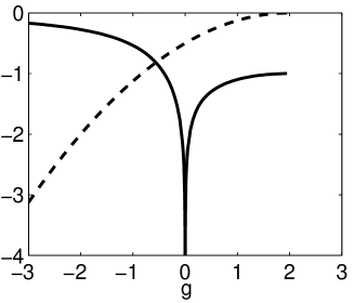
Figure 6: Dependence of the chemical potential $\mu$ ($--$) and the parameter $x_{0}$ (—) on the nonlinearity $g\leq g_{c}=2$ for the bound state of the nonlinear Schrödinger equation for an attractive delta potential $V(x)=-\delta(x)$.

The dependence of $x_{0}$ and $\mu$ on the nonlinearity $g$ is illustrated in figure 6. The position $x_{0}$ is given by equation (8) for $g<0$ and (20) for $g>0$, however with $k=-\lambda-g/2$.

For $g=0$, one finds the well–known value $\mu=-\lambda^{2}/2$, whereas the function $x_{0}(g)$ has a logarithmic singularity. Nevertheless, the bound state wavefunction $\psi(x)$ evolves smoothly into the well–known bound state (6) of the linear problem for an attractive as well as a repulsive nonlinearity.

For $g\rightarrow g_{c}=-2\lambda$, the chemical potential $\mu$ tends to zero and $x_{0}$ tends to the finite value $1/\lambda$. The disappearance of the bound state if $g$ is increased above $g_{c}$ is similar to the effect observed by Moiseyev et al. [10] for a smooth potential $V(x)$ where a bound state is transformed into a resonance–like state at a critical nonlinear interaction.

3 Delta–shell potential

In this section we discuss another simple and very popular model system: the delta–shell potential. A detailed discussion of the linear three–dimensional delta–shell potential can be found in [11]. Here we restrict ourselves to the one–dimensional case

$$V(x)=\left\{\begin{array}[]{*{2}{l}}+\infty&\mbox{for}\,x<0\\ \lambda\delta(x-a)&\mbox{for}\,x\geq 0\\ \end{array}\right.$$ (32)

with $a>0$. First we briefly resume the basic features of the delta–shell potential in the linear case ($g=0$), in particular the existence of bound states in an attractive potential and resonances in a repulsive one. As we have already discussed the properties of bound states in a single delta potential in some detail, we now concentrate on the case of a repulsive potential ($\lambda>0$). We set $\hbar=1$ and $m=1$ as above.

3.1 The linear case

In the linear case $g=0$, the wavefunction in a delta–shell potential is given by

$$\psi_{k}(x)=\left\{\begin{array}[]{*{2}{l}}\sin(kx)&\mbox{for}\;x<a\\[5.69054pt] \sin(kx)+\frac{2\lambda}{k}\sin(ka)\sin(k(x-a))&\mbox{for}\;x>a,\\ \end{array}\right.$$ (33)

The phase shift $\delta(k)$ between incoming and outgoing waves for $x>a$ is easily calculated and yields

$$\tan\delta(k)=\frac{\cos(2ka)-1}{\sin(2ka)+k/\lambda}\,.$$ (34)

The S–matrix $S(k)$ is defined in terms of the the phase shift $\delta(k)$ by [12]:

$$S(k)=\frac{1+{\rm i}\tan\delta(k)}{1-{\rm i}\tan\delta(k)}\,.$$ (35)

Bound states correspond to poles of the S–Matrix $S(k)$ on the positive imaginary axis. Calculating these poles one arrives at

$${\rm e}^{2{\rm i}ka}=1-\frac{{\rm i}k}{\lambda}\,.$$ (36)

This equation has a solution on the positive imaginary axis if the condition

$$\lambda a>-\,\frac{1}{2}$$ (37)

is fulfilled. This implies that the delta–shell potential has to be sufficiently attractive to support a bound state. If the distance $a$ is reduced or $\lambda$ is increased, so that the condition (37) is not fulfilled any longer, the bound state is lost and one finds a virtual state instead. A virtual state corresponds to a pole of the S–matrix $S(k)$ on the negative imaginary axis [12]. The wavefunction of such a state diverges exponentially. For $a\rightarrow\infty$ the delta–shell potential is equivalent to a single delta potential and the energy is $E\rightarrow-\lambda^{2}/2$.

Naturally there exist no bound states in a repulsive delta–shell potential, but one can find resonance states. A resonance is defined by a pole of the S–matrix $S(k)$ in the lower half plane [12]. The energy of the n–th resonance is also complex

$${\cal E}_{n}=k_{n}^{2}/2=E_{n}-{\rm i}\Gamma_{n}/2,$$ (38)

where the imaginary part $\Gamma_{n}$ is interpreted as a decay rate. In the vicinity of a resonance, the phase shift $\delta(k)$ rapidly changes by an amount of $\pi$.

The amplitude of a resonance wavefunction is enhanced for $x<a$. This is illustrated in figure 7 for a delta–shell potential of strength $\lambda=10$ at $a=1$. The ratio of the amplitudes on the left–hand side ($x<a$) and on the right–hand side ($x>a$) of the delta–shell potential, denoted as $A_{l}$ resp. $A_{r}$, is plotted for real values of the energy. The peaks of the amplitude ratio $A_{l}/A_{r}$ close to the resonances are clearly visible. The squared modulus of the wavefunction of the most stable resonance at ${\cal E}_{1}=4.488-0.063{\rm i}$ is displayed on the right. Nevertheless one has to keep in mind that the wavefunction finally diverges exponentially for complex energies ${\cal E}$, whereas it is periodic for real energies.

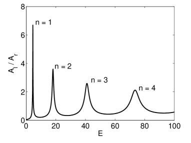
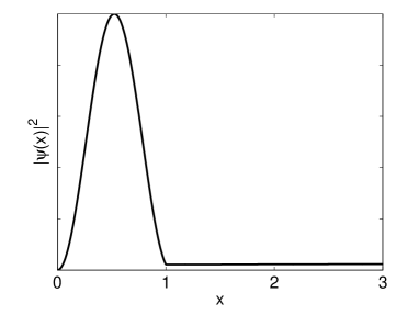
Figure 7: Left: Amplitude ratio $A_{l}/A_{r}$ for a delta–shell potential with $a=1$ and $\lambda=10$ in the linear case. Right: Squared modulus of the wavefunction of the most stable resonance at ${\cal E}_{1}=4.488-0.063{\rm i}$.

3.2 Resonances in the nonlinear case

Now we come back to the nonlinear Schrödinger equation

$$\left(-\frac{1}{2}\frac{{\rm d}^{2}}{{\rm d}x^{2}}+\lambda\delta(x-a)+g|\psi(x)|^{2}\right)\psi(x)=\mu\,\psi(x)\quad\mbox{for}\quad x\geq 0.$$ (39)

In the following we will only discuss the case of a repulsive delta–shell potential ($\lambda>0$). By means of a scaling $x=x^{\prime}/s$, $\psi=\psi^{\prime}\sqrt{s}$, $\lambda=\lambda^{\prime}s$ and $\mu=\mu^{\prime}s^{2}$ for $s>0$ (which conserves the normalization), the number of independent parameters is reduced to two. As we are mainly interested in the effects of a varying nonlinearity, the potential is fixed by $a=1$ and $\lambda=10$ in the following examples. In the linear case we find resonances for this potential. Now we want to identify and characterize resonances in the nonlinear case as well.

But the definition of a resonance becomes somewhat ambitious in the nonlinear case. A decomposition into incoming and outgoing waves and thus a definition of the S–matrix $S(k)$ is not possible. One method widely used to compute resonances in the linear case is exterior complex scaling (see e.g. [13]). This technique has also been successfully applied to the nonlinear Schrödinger equation [10, 14].

We will not adopt this approach but rather look for solutions that can be expressed analytically. We have already learned that the real solutions of the free nonlinear Schrödinger equation are given in terms of Jacobi elliptic functions. These solutions are matched at $x=a$ to obtain solutions for the delta–shell potential. The chemical potential $\mu$ of such a solution is real. Thus we can define a resonance neither by a complex eigenenergy nor via the S–matrix. In the following we will rather call a state a resonance, when its amplitude is resonantly enhanced in the vicinity of the potential, i.e. for $x<a$.

Let us briefly discuss the time evolution of nonlinear resonances. Note that the states

$$\psi(x,t)=\exp(-{\rm i}\mu t)\,\psi(x)$$ (40)

with a complex chemical potential $\mu=\mu_{r}-{\rm i}\Gamma/2$ do not fulfill the time–dependent nonlinear Schrödinger equation, because the norm of these states is not constant. One can circumvent this problem by introducing an additional source term or one considers the states (40) just as an adiabatic approximation [14]. On the contrary the states (40) with a real chemical potential $\mu$ discussed in this paper fulfill the time–dependent nonlinear Schrödinger equation but do not decay.

Furthermore we have to be cautious about the nonlinear parameter $g$. A meaningful definition of the nonlinearity requires that the norm or the amplitude of a solution must be fixed in some way, e.g. by $\|\psi\|=1$ in section 2. This is not applicable any longer since resonance states are not normalizable. As a global measure of the nonlinear interaction we thus define the mean–field potential $g|\psi(x)|^{2}$, integrated over the ”interaction–region” $0<x<a$ of the external potential:

$$g_{\rm eff}=g\int_{0}^{a}|\psi(x)|^{2}\,{\rm d}x\,.$$ (41)

3.3 Attractive Nonlinearity

First we discuss the nonlinear Schrödinger equation with a negative nonlinearity $g$, corresponding to an attractive mean–field interaction. As stated above, the real–valued periodic solutions of the free nonlinear Schrödinger equation with a negative nonlinearity can be expressed in terms of the Jacobi elliptic function cn [6, 7]. Thus, in order to find solutions for the delta–shell potential we make an ansatz of the form (26) separately for $x<a$ and $x>a$:

$$\psi(x)=\left\{\begin{array}[]{l}\psi_{l}(x)=A_{l}\,{\rm cn}\Big{(}4K(p_{l})\big{(}\frac{x}{L_{l}}+\frac{1}{4}\big{)}\,\Big{|}\,p_{l}\Big{)}\quad\mbox{for}\;x<a\\[5.69054pt] \psi_{r}(x)=A_{r}\,{\rm cn}\Big{(}4K(p_{r})\frac{x+x_{0}}{L_{r}}\,\Big{|}\,p_{r}\Big{)}\qquad\mbox{for}\;x>a.\end{array}\right.$$ (42)

The amplitudes $A_{l,r}$ and the periods $L_{l,r}$ are given by

$$A_{l,r}=\frac{4\,\sqrt{p_{l,r}}\,K(p_{l,r})}{\sqrt{|g|}\,L_{l,r}}\quad\mbox{and}\quad\mu=\frac{8\,(1-2p_{l,r})\,K(p_{l,r})^{2}}{L_{l,r}^{2}}\,,$$ (43)

where $p_{l,r}$ are the elliptic parameters of the solution on the left–hand ($x<a$) and on the right–hand ($x>a$) side of the delta–shell. Clearly one has only one value for the chemical potential, whereas the amplitude $A$, the parameter $p$ and the period $L$ generally differ for $x<a$ and $x>a$. This is different from the linear case, where the period $L$ is fixed with the energy. The chemical potential is positive, $\mu\geq 0$, if the elliptic parameter is restricted to $p_{l,r}\in[0,1/2]$.

The boundary condition $\psi(0)=0$ is automatically fulfilled by this ansatz. Furthermore the wavefunction must be continuous at $x=a$, whereas its derivative is discontinuous according to equation (5), leading to the conditions:

$${\rm I.}\qquad A_{l}\,{\rm cn}(u_{l}|p_{l}) = A_{r}\,{\rm cn}(u_{r}|p_{r})$$ (44)

$${\rm II.}\quad 2\lambda A_{l}\,{\rm cn}(u_{l}|p_{l}) = -\frac{4A_{r}K_{r}}{L_{r}}{\rm sn}(u_{r}|p_{r}){\rm dn}(u_{r}|p_{r})+\frac{4A_{l}K_{l}}{L_{l}}{\rm sn}(u_{l}|p_{l}){\rm dn}(u_{l}|p_{l}),$$ (45)

where the abbreviations $u_{l}=K(p_{l})(4a/L_{l}+1)$ and $u_{r}=4K(p_{r})(a+x_{0})/L_{r}$ have been used. The first condition can be fulfilled by an appropriate choice of $x_{0}$, as long as $|A_{l}\,{\rm cn}(u_{l}|p_{l})|\leq|A_{r}|$. Then one can insert the first condition into the second one and arrives at

$$\frac{2\lambda^{2}}{\mu}\frac{p_{l}}{1-2p_{l}}{\rm cn}(u_{l}|p_{l})^{2}-\frac{4\lambda}{\sqrt{2\mu}}\frac{p_{l}}{(1-2p_{l})^{3/2}}\,{\rm cn}(u_{l}|p_{l}){\rm dn}(u_{l}|p_{l}){\rm sn}(u_{l}|p_{l})$$

$$=\frac{(1-p_{r})p_{r}}{(1-2p_{r})^{2}}-\frac{(1-p_{l})p_{l}}{(1-2p_{l})^{2}}\,.$$ (46)

As argued above we are looking for solutions whose amplitudes are resonantly enhanced for $x<a$, i.e. for solutions with a maximum amplitude ratio $A_{l}/A_{r}$. This ratio is given directly by the elliptic parameters $p_{l,r}$:

$$\frac{A_{l}}{A_{r}}=\left[\frac{p_{l}(1-2p_{r})}{(1-2p_{l})p_{r}}\right]^{1/2}.$$ (47)

A resonant enhancement of the amplitude ratio demands that $p_{l}\gg p_{r}$.

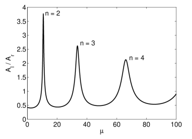
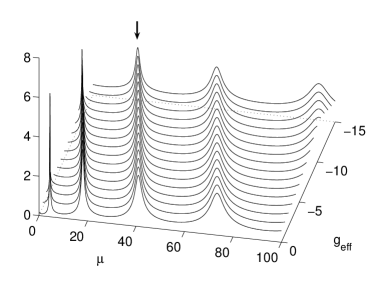
Figure 8: Amplitude ratio $A_{l}/A_{r}$ as a function of the chemical potential $\mu$ for an effective nonlinearity $g_{\rm eff}=-5$ (left) and for different effective nonlinearities $g_{\rm eff}$ (right). The shift of the resonance marked by an arrow is displayed as a function of $g_{\rm eff}$ in figure 9.

In order to identify and analyze resonances of the nonlinear Schrödinger equation we now calculate the amplitude ratio $A_{l}/A_{r}$ as a function of the the chemical potential for different values of the effective nonlinearity $g_{\rm eff}$. The left–hand side of figure 8 shows the amplitude ratio as a function of $\mu$ for an effective nonlinearity $g_{\rm eff}=-5$. As in the linear case, illustrated in figure 7, resonances can be clearly identified as maxima of the amplitude ratio $A_{l}/A_{r}$. The resonances are, however, shifted to smaller values of $\mu$, whereas the width of the resonances remains similar.

On the right–hand side of figure 8 the amplitude ratio $A_{l}/A_{r}(\mu)$ is plotted for different values of the effective nonlinearity $g_{\rm eff}$. Resonances are clearly identified for all values of $g_{\rm eff}$, but the shift of the resonance positions is clearly visible in this illustration. We note that the resonance heights barely change with $g_{\rm eff}$.

The observed shift of the resonances will be explained in the following. For convenience we rather calculate the chemical potential where $A_{l}=A_{r}$ at the sides of each resonance, in dependence of $g_{\rm eff}$. These values of the chemical potential will be denoted $\mu_{n}^{<}$ and $\mu_{n}^{>}\,$ in the following. They are easier to calculate than the resonance positions $\mu_{n}$ because $p_{l}=p_{r}$ holds at these values, furthermore this calculation will also reveal the influence of $g_{\rm eff}$ on the resonance width. We note that the wavefunction on the interval $x\in[0,2a]$ is symmetric (antisymmetric) around $x=a$ for $\mu=\mu_{n}^{<}$ ($\mu=\mu_{n}^{>}$).

Using both equations (43), the chemical potential can be written as

$$\mu=gA^{2}\left(1-\frac{1}{2p}\right).$$ (48)

The elliptic parameter $p$ can be calculated from the relation

$$pK(p)^{2}=\frac{|g|A^{2}L^{2}}{16}.$$ (49)

Solving this relation for $p$ leads to

$$p=\frac{|g|A^{2}L^{2}}{4\pi^{2}}-\frac{1}{2}\left(\frac{|g|A^{2}L^{2}}{4\pi^{2}}\right)^{2}+\mathcal{O}(g^{3}A^{6})\,,$$ (50)

and inserting this into equation (48), we find the desired dependence of the chemical potential on the nonlinear interaction

$$\mu=\frac{2\pi^{2}}{L^{2}}\left(1+\frac{3gA^{2}L^{2}}{8\pi^{2}}+\mathcal{O}(g^{2}A^{4}))\right).$$ (51)

Formula (51) is valid for both $\mu_{n}^{>}$ and $\mu_{n}^{<}$. Now we insert the specific values of the period $L$ and replace $gA^{2}$ by the effective nonlinearity $g_{\rm eff}$. At $\mu_{n}^{>}$ the period of the wavefunction is $L_{n}^{>}=2a/n$, i.e. $\psi(a)=0$. Equation (41) for the effective nonlinearity can be easily evaluated in lowest order in $p$, since then the elliptic function cn equals a cosine, which yields $g_{\rm eff}\approx gA^{2}a/2$. This finally leads to

$$\mu_{n}^{>}\approx\frac{n^{2}\pi^{2}}{2a^{2}}+\frac{3g_{\rm eff}}{2a}\,.$$ (52)

Similarly one obtains an expression for $\mu_{n}^{<}$. In the linear case the period $L_{n}^{<}$ is given by the solution of the implicit equation

$$\tan\left(\frac{2\pi a}{L_{n}^{<}}\right)=-\frac{2\pi}{\lambda L^{<}_{n}}.$$ (53)

For the example illustrated in figure 9 ($a=1$, $\lambda=10$ and $n=3$) one has $L_{3}^{<}=0.7215$ . The change of $L_{n}^{<}$ with $g_{\rm eff}$ is negligible. Again equation (41) for the effective nonlinearity is readily evaluated in lowest order in $p$ and yields

$$g_{\rm eff} \approx \frac{gaA^{2}}{2}\left(1-\frac{\sin(4\pi a/L_{n}^{<})}{4\pi a/L_{n}^{<}}\right)=\frac{gaA^{2}}{2}\left(1+\frac{1}{\lambda a(1+(2\pi)^{2}/(\lambda L_{n}^{<})^{2})}\right).$$ (54)

Inserting into equation (51), one finally arrives at

$$\mu_{n}^{<}\approx\frac{2\pi^{2}}{(L_{n}^{<})^{2}}+\frac{3g_{\rm eff}}{2a}\left(1-\frac{\sin(4\pi a/L_{n}^{<})}{4\pi a/L_{n}^{<}}\right)^{-1}\,.$$ (55)

The same results are obtained in the case of a repulsive interaction ($g>0$, see below). Thus we compare the approximations (52) and (55) to the numerically exact results for $g<0$ and $g>0$ together in figure 9. We considered the resonance with $n=3$, that is marked with an arrow in the figures 8 and 10. We observe a good agreement. Furthermore the positions $\mu_{n=3}$ of the resonances are displayed.

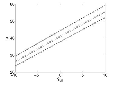
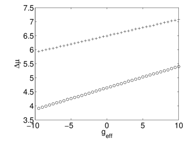
Figure 9: Left: Dependence of the resonance position $\mu_{n}$ (o) and $\mu^{>}_{n}$ (+) and $\mu^{<}_{n}$ (x) on the effective nonlinearity $g_{\rm eff}$ for $n=3$. The solid lines are the approximations (52) and (55). Right: Width of the resonance, defined as $\Delta\mu=\mu_{3}^{>}-\mu_{3}^{<}$ (+) and as FWHM (o).

From the different scaling of $\mu_{n}^{>}$ and $\mu_{n}^{<}$ we conclude that the resonance width also changes with the effective nonlinearity. In fact, the width increases almost linearly with $g_{\rm eff}$ and the resonances become slightly asymmetric. The dependence of the width $\Delta\mu=\mu_{3}^{>}-\mu_{3}^{<}$ on the effective nonlinearity $g_{\rm eff}$ is illustrated in figure 9 on the right.

It should not be concealed that also bound stated can exist in a repulsive delta–shell potential due to the attractive self–interaction, falling of as ${\rm sech}\big{(}\sqrt{-2\mu}(x-x_{0})\big{)}$ for $x>a$. However we will not consider these states here as we already discussed a similar phenomenon for the single delta potential.

3.4 Repulsive Nonlinearity

As stated above, the real non–singular solutions of the free nonlinear Schrödinger equation with a repulsive nonlinearity can be expressed in terms of the Jacobi elliptic function sn [8, 7]. Thus we make the ansatz:

$$\psi(x)=\left\{\begin{array}[]{l}\psi_{l}(x)=A_{l}\,{\rm sn}\bigg{(}4K(p_{l})\frac{x}{L_{l}}\bigg{|}p_{l}\bigg{)}\quad\mbox{for}\;x<a\\[5.69054pt] \psi_{r}(x)=A_{r}\,{\rm sn}\bigg{(}4K(p_{r})\frac{x+x_{0}}{L_{r}}\bigg{|}p_{r}\bigg{)}\quad\mbox{for}\;x>a.\end{array}\right.$$ (56)

The amplitudes $A_{l,r}$ and the periods $L_{l,r}$ are now given by

$$A_{l,r}=\frac{4\,\sqrt{p_{l,r}}\,K(p_{l,r})}{\sqrt{|g|}\,L_{l,r}}\quad\mbox{and}\quad\mu=\frac{8(p_{l,r}+1)\,K(p_{l,r})^{2}}{L_{l,r}^{2}},$$ (57)

where $p_{l,r}\in[0,1]$ are the elliptic parameters of the solution on the left ($x<a$) and on the right ($x>a$) of the delta–shell.

The boundary condition $\psi(0)=0$ is automatically fulfilled by the ansatz (56). The remaining conditions for the wavefunction and its derivative at $x=a$ (cf. equation (5)) read:

$${\rm I.}\qquad A_{l}\,{\rm sn}(u_{l}|p_{l}) = A_{r}\,{\rm sn}(u_{r}|p_{r})$$ (58)

$${\rm II.}\quad 2\lambda A_{l}\,{\rm sn}(u_{l}|p_{l}) = \frac{4A_{r}K_{r}}{L_{r}}{\rm cn}(u_{r}|p_{r}){\rm dn}(u_{r}|p_{r})-\frac{4A_{l}K_{l}}{L_{l}}{\rm cn}(u_{l}|p_{l}){\rm dn}(u_{l}|p_{l}),$$ (59)

where the abbreviations $u_{l}=4K(p_{l})a/L_{l}$ and $u_{r}=4K(p_{r})(a+x_{0})/{L_{r}}$ have been used.

If $|A_{l}{\rm sn}(u_{l}|p_{l})|\leq|A_{r}|$ the first condition can always be fulfilled by an appropriate choice of the ”phase shift” $x_{0}$. Inserting the first condition into the second one and using the addition theorems of the Jacobi elliptic functions one arrives at

$$\frac{2\lambda^{2}}{\mu}\frac{p_{l}}{p_{l}+1}{\rm sn}^{2}(u_{l}|p_{l})+\frac{p_{l}}{(p_{l}+1)^{3/2}}\frac{4\lambda}{\sqrt{2\mu}}{\rm cn}(u_{l}|p_{l}){\rm dn}(u_{l}|p_{l}){\rm sn}(u_{l}|p_{l})$$

$$=\quad\frac{p_{r}}{(p_{r}+1)^{2}}-\frac{p_{l}}{(p_{l}+1)^{2}}\,.$$ (60)

The amplitude ratio $A_{l}/A_{r}$ is given by

$$\frac{A_{l}}{A_{r}}=\left[\frac{p_{l}(p_{r}+1)}{(p_{l}+1)p_{r}}\right]^{1/2}$$ (61)

in terms of the elliptic parameters. A resonant enhancement of the amplitude ratio demands that $p_{l}\gg p_{r}$.

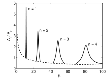
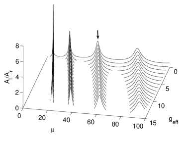
Figure 10: Left: Amplitude ratio as a function of the chemical potential $\mu$ for an effective nonlinearity $g_{\rm eff}=5$. The condition (63) for the amplitude ratio is plotted as a dashed line. Right: Amplitude ratio as a function of the chemical potential $\mu$ for different effective nonlinearities. The shift of the resonance marked with an arrow is displayed as a function of $g_{\rm eff}$ in figure 9.

Again we calculated the amplitude ratio $A_{l}/A_{r}$ as a function of the chemical potential $\mu$ for different values of the effective nonlinearity $g_{\rm eff}$. The results are illustrated in figure 10. The left–hand side shows the amplitude ratio $A_{l}/A_{r}$ for an effective nonlinearity $g_{\rm eff}=5$, what should be compared to figure 7 and figure 8. The first observation is that one cannot find solutions for all values of $\mu$. In fact there exist no solutions with an amplitude ratio below a certain threshold. Resonances are still clearly identified as maxima of the amplitude ratio. Again the resonance positions are shifted in comparison to the linear case.

On the right–hand side the amplitude ratio is plotted for different values of $g_{\rm eff}$. One observes that the solutions cease to exist with an increasing effective nonlinearity, whereas the resonances survive longest. The resonances are shifted similarly to the case of an attractive interaction.

Solutions with a small amplitude ratio $A_{l}/A_{r}$ cease to exist when $g_{\rm eff}$ is increased. In fact, condition (59) cannot be fulfilled any longer if the amplitude ratio $A_{l}/A_{r}$ drops below a certain threshold. A condition for the existence of a solution can be derived from the equations (61) and (57) and yields

$$\left(\frac{A_{l}}{A_{r}}\right)^{2}\geq\frac{2p_{l}}{p_{l}+1}=\frac{gA_{l}^{2}}{\mu}\,.$$ (62)

Inserting $g_{\rm eff}\approx gaA_{l}^{2}/2$ on the right hand side, one is led to the approximation

$$\frac{A_{l}}{A_{r}}\apprge\left(\frac{2\,g_{\rm eff}}{a\mu}\right)^{1/2}\,.$$ (63)

As a consequence solutions apart of the resonances with small amplitude ratios cease to exist when $g_{\rm eff}$ is increased. This approximate condition is well confirmed by the numerical exact results displayed in figure 10.

The shift of the resonances is understood in the same way as in the case of an attractive interaction. The chemical potential is now given by

$$\mu=gA^{2}\left(\frac{1}{2}+\frac{1}{2p}\right),$$ (64)

while equation (50) still holds. Inserting into equation (64) and expanding up to the linear term in $gA^{2}$ again leads to equation (51). Thus one arrives at the same results as in the case of an repulsive interaction, in particular at the equation (52) for $\mu_{n}^{>}$ and equation (55) for $\mu_{n}^{<}$. The results for $n=3$ are displayed in figure 9. The approximations agree well with the numerical exact results. From the different scaling of $\mu_{n}^{>}$ and $\mu_{n}^{<}$ with $g_{\rm eff}$ we conclude that a repulsive nonlinearity increases the resonance width.

4 Conclusion

In this paper we analyzed the properties of bound, scattering and resonance states of the nonlinear Schrödinger equation using two simple model systems.

Bound, i.e. normalizable, states were calculated and analyzed for a single delta potential. New features occur in the case of an attractive nonlinearity, as states are no longer bound by an external potential but by the internal interaction. In this case bound states can exist despite a repulsive external potential, and they cease to exist at a negative value of the chemical potential. In addition we investigated the transition from bound to scattering states.

Furthermore we discussed a repulsive delta–shell potential as a simple model showing resonances. Resonances can still be identified in the nonlinear case, though the definition of a resonance becomes somewhat ambitious. Two major effects of the nonlinearity were analyzed in detail: Firstly, the resonance positions are shifted proportionally to the effective nonlinearity and the resonance width increases with $g_{\rm eff}$. Secondly, scattering states cease to exist with an increasing repulsive nonlinearity, whereas resonances survive longest.

References

References

- [1] E. M. Lifshitz and L. P. Pitaevskii, Statistical Physics, Part II, Pergamon, Oxford, 1980
- [2] M. Greiner, I. Bloch, O. Mandel, T. W. Hänsch, and T. Esslinger, Appl. Phys. B 73 (2001) 769
- [3] R. K. Dodd, J. C. Eilbeck, J. D. Gibbon, and H. C. Morris, Solitons and nonlinear wave equations, Academic Press, London, 1982
- [4] V. Hakim, Phys. Rev. E 55 (1997) 2835
- [5] P. Leboeuf and N. Pavloff, Phys. Rev. A 64 (2001) 033602
- [6] L. D. Carr, C. W. Clark, and W. P. Reinhardt, Phys. Rev. A 62 (2000) 063611
- [7] R. D’Agosta, B.A. Malomed, and C. Presilla, Phys. Lett. A 275 (2000) 424
- [8] L. D. Carr, C. W. Clark, and W. P. Reinhardt, Phys. Rev. A 62 (2000) 063610
- [9] M. Abramowitz and I. A. Stegun, Handbook of Mathematical Functions, Dover Publications, Inc., New York, 1972
- [10] N. Moiseyev, L. D. Carr, B. A. Malomed, and Y. B. Band, J. Phys. B (2004) L193
- [11] K. Gottfried, Quantum Mechanics, Benjamin, New York, 1966
- [12] J. R. Taylor, Scattering Theory, John Wiley, New York, 1972
- [13] N. Moiseyev, Phys. Rep. 302 (1998) 211
- [14] P. Schlagheck and T. Paul, cond-mat/0402089 (2004)