Nonlinear quantum optical computing via measurement.

Abstract

We show how the measurement induced model of quantum computation proposed by Raussendorf and Briegel [Phys. Rev. Letts. 86, 5188 (2001)] can be adapted to a nonlinear optical interaction. This optical implementation requires a Kerr nonlinearity, a single photon source, a single photon detector and fast feed forward. Although nondeterministic optical quantum information proposals such as that suggested by KLM [Nature 409, 46 (2001)] do not require a Kerr nonlinearity they do require complex reconfigurable optical networks. The proposal in this paper has the benefit of a single static optical layout with fixed device parameters, where the algorithm is defined by the final measurement procedure.

PACS numbers: 03.67.-a

Introduction

Raussendorf and Briegel [1] have shown how efficient quantum computation can be implemented on an array of suitably entangled qubits using a sequence of measurements and conditional unitary operations conditioned on the measurement results. Their scheme was based on an array of interacting spins described by the Ising Hamiltonian and is thus applicable to certain solid state implementations. In this paper we show that a similar scheme can be used in a quantum optical computer based on a mutual Kerr interaction between optical field modes excited with single photon states. This interaction was long ago suggested as a possible path to implementing quantum gates in optics [2, 3]. While the mutual Kerr interaction is likely to become a central component in all-optical communication schemes [4, 5, 6], the currently available technology cannot produce mutual Kerr interactions sufficiently large to enable single photon operation. Given sufficient motivation however one might expect that this technological challenge could be answered and we consider it worthwhile to investigate simple schemes of all-optical quantum computation that requires such a nonlinearity. In any case the model we describe shows that the scheme of Raussendorf and Briegel can be implemented in principle in an all optical network.

We begin with a brief summary of the scheme in reference [1]. In section 2 we present a dual rail logical code for qubits based on one photon and two modes per qubit. This code was recently used by Knill et al. [7] to show that linear efficient quantum computation can be done with linear optics and single photons provided efficient single photon measurement and fast feed forward control can be implemented. The scheme we describe here also uses measurement and feed forward, but requires a nonlinear interaction. In section 3 we discuss the practicality of the scheme and end with a short conclusion.

1 Quantum computing via measurement.

In order to fix concepts and notation we begin with a brief description of the Raussendorf and Briegel scheme [1]. This scheme consists of a protocol for teleportation and the implementation of a controlled not gate (CNOT), where the manipulation of single qubits via unitary operations are assumed. Consider an array of qubits that interact via the Ising nearest neighbour interaction,

$$\mathcal{H}=-\frac{1}{4}g(t)\sigma_{z}^{(1)}\sigma_{z}^{(2)}.$$ (1)

where $\sigma_{z}^{(i)}$ is the Pauli matrix diagonal in the logic code (computational) basis $|0\rangle,|1\rangle$. Here the strength $g(t)$ can be controlled externally. If the array begins as a product state in the logic basis, this interaction cannot create entanglement. If however we initialise the array as a product state of $\sigma_{x}^{(i)}$ eigenstates, $|+\rangle=1/\sqrt{2}(|0\rangle+|1\rangle)$ for each qubit, entanglement can be created if the Ising interaction is turned on for a certain time, thus applying the unitary operator

$$S=\exp({-i\mathcal{H}_{int}(t)}).$$ (2)

This initialisation procedure requires only single qubit rotations, which we assume can be easily implemented. We also note that for this entangling procedure Raussendorf and Briegel in their scheme used the Hamiltonian

$$\mathcal{H}_{\mathrm{int}}=g(t)\sum_{\langle a,a^{\prime}\rangle}\frac{1+{\sigma_{z}}^{(a)}}{2}\frac{1+{\sigma_{z}}^{(a^{\prime})}}{2}.$$ (3)

Instead we have used an equivalent but different form

$$\mathcal{H}_{\mathrm{int}}=-\frac{1}{4}g(t)\sum_{\langle a,a^{\prime}\rangle}{\sigma_{z}}^{(a)}{\sigma_{z}}^{(a^{\prime})},$$ (4)

in order to implement this entangling operation in our nonlinear quantum optical computing via measurement scheme.

The time necessary to maximally entangle the qubits can be found by taking the partial trace over the first qubit, in a two qubit system. This result generalises to many qubits. If we take the input state $|\psi\rangle_{in}=|+\rangle_{1}\otimes|+\rangle_{2}$, apply the unitary operator $U(\theta)=\exp({-i\theta\sigma_{z}^{(1)}\sigma_{z}^{(2)}})$ and take the partial trace over the second qubit; we have the state

$$\rho^{(1)}=\phantom{+}|0\rangle\langle 0|+|1\rangle\langle 1|+2\cos(2\theta)[|1\rangle\langle 0|+|0\rangle\langle 1|].$$ (5)

Clearly the qubits are maximally entangled when $\theta=\pi/4$.

To transport an arbitrary state $|\psi_{\mathrm{in}}\rangle=\alpha|0\rangle+\beta|1\rangle$ across three or more of the qubits we employ the following protocol:

1. We take a chain of an odd number of qubits and prepare them in the state $|\psi_{\mathrm{in}}\rangle_{1}\otimes|+\rangle_{2}\otimes\ldots\otimes|+\rangle_{n}$ and entangle the qubits by applying the unitary operation $S=\exp\left({-i\frac{\pi}{4}\sum_{\langle a,a^{\prime}\rangle}\sigma_{z}^{(a)}\sigma_{z}^{(a^{\prime})}}\right)$.

2. To teleport the state, $\sigma_{x}$ measurements are made sequentially on the first qubit through to the second last qubit. The process yields the measurement outcomes $s_{j}\in\{0,1\}$ for all but the last qubit. These outcomes correspond to the qubits being in the states $|+\rangle=|0\rangle_{x}$ and $|-\rangle=|1\rangle_{x}$ respectively. The final state of the system after the $(n-1)$ $\sigma_{x}$ measurements place the system in the state $|s_{1}\rangle_{1}\otimes|s_{2}\rangle_{2}\otimes\ldots\otimes|s_{n-1}\rangle_{n-1}\otimes|\psi_{\mathrm{out}}\rangle_{n}$.

3. The output state $|\psi_{\mathrm{out}}\rangle$ is related to the input state $|\psi_{\mathrm{in}}\rangle$ by a unitary transformation $U_{\mathrm{teleport}}\in\{1,\sigma_{x},\sigma_{z},\sigma_{x}\sigma_{z}\}$ determined by the set of measurement outcomes $\{s_{1},s_{2},\ldots,s_{n-1}\}$.

For the case of teleporting over three qubits we find for the measurement outcomes $\{|-\rangle,|-\rangle\}$, $\{|+\rangle,|+\rangle\}$, $\{|+\rangle,|-\rangle\}$ and $\{|+\rangle,|-\rangle\}$ on the first and second qubits require the unitary operations $1$, $\sigma_{x}$, $\sigma_{z}$ and $\sigma_{x}\sigma_{z}$ respectively.

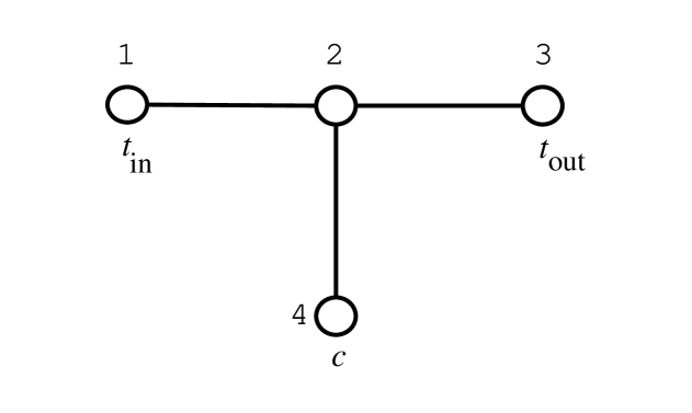
Figure 1: CNOT gate configuration. The CNOT consists of four qubits, and uses the measurement of qubits one and two to project an output state to qubit three. This state is a known unitary transformation from the desired CNOT target state, defined by the two measurement results. The CNOT input state $t_{\mathrm{in}}$ is at qubit one and the output state $t_{\mathrm{out}}$ is at qubit three. The control state $c$ is at qubit four.

By making appropriate measurements on an array of four qubits, entangled by this scheme, it is possible to implement a particular universal two qubit gate, the CNOT gate. Consider the two dimensional array shown in figure 1. The control qubit, is labelled $c$ while the target qubits is labelled $t$. In this scheme the physical system coding the target qubit will change. We allow for this by the notation $t_{in},t_{out}$. In a CNOT gate, the logical state of the control does not change. However if the logical state of the control is $1$ the logical state of the target qubit is inverted. If the logical state of the qubit is $0$, the logical state of the target is not changed.

[Insert figure 1 about here ]

To implement this gate we place four qubits in the configuration of figure 1. Each qubit is a node in this graph while non-zero nearest neighbour interactions are indicated by edges. Qubit four is the control. During the operation of the CNOT in this scheme, qubit $c$ acts as the site where the control state is input and output at the end of the gate operation. The information state is input onto qubit $t_{\mathrm{in}}$ and after the gate operation has completed we have the desired state output to qubit $t_{\mathrm{out}}$. Our operation of the CNOT gate is as follows:

1. We prepare the states on qubit one and four, these are $|i_{1}\rangle_{1}$ and $|i_{4}\rangle_{4}$ respectively, where $i_{1}$ and $i_{4}\in\{0,1\}$. The other two qubits are prepared in eigenstates of $\sigma_{x}$ with positive eigenvalue, $|+\rangle$. Thus the initial state of the CNOT gate is

   $$|\psi_{\mathrm{in}}\rangle=|i_{1}\rangle_{1}\otimes|+\rangle_{2}\otimes|+\rangle_{3}\otimes|i_{4}\rangle_{4}\ .$$ (6)

2. We entangle the four qubits by turning on the Ising interaction between the connected neighbouring sites for an appropriate amount of time $\pi/4$. This transforms the initial state of the qubits according to the evolution operator

   $$S=\exp\left({-i\frac{\pi}{4}\left(\sigma_{z}^{(1)}\sigma_{z}^{(2)}+\sigma_{z}^{(2)}\sigma_{z}^{(3)}+\sigma_{z}^{(2)}\sigma_{z}^{(4)}\right)}\right).$$ (7)

   By entangling the qubits we produced the state

   $$S|\psi_{\mathrm{in}}\rangle = \phantom{+}\exp\left({-i\frac{\pi}{4}((-1)^{i_{1}}+(-1)^{i_{4}}+1)}\right)|i_{1}00i_{4}\rangle$$ (8)

   $$+\exp\left({-i\frac{\pi}{4}((-1)^{i_{1}}+(-1)^{i_{4}}-1)}\right)|i_{1}01i_{4}\rangle$$

   $$+\exp\left({-i\frac{\pi}{4}((-1)^{1-i_{1}}+(-1)^{1-i_{4}}-1)}\right)|i_{1}10i_{4}\rangle$$

   $$+\exp\left({-i\frac{\pi}{4}((-1)^{1-i_{1}}+(-1)^{1-i_{4}}+1)}\right)|i_{1}11i_{4}\rangle,$$

   where we have used a more compact notation using the four digits in the ket as a representation for the each of the four qubits states ordered from qubit 1 to 4.

3. To output the correct state at qubit three, a $\sigma_{x}$ measurement is made on qubit one and then another measurement on qubit two. The measurement outcomes are labelled, $s_{j}\in\{0,1\}$.

4. Finally, the output state of the system after the two measurements in the $\sigma_{x}$ basis is

   $$|\psi_{\mathrm{out}}\rangle=|s_{1}\rangle_{1}\otimes|s_{2}\rangle_{2}\otimes U_{\mathrm{CNOT}}|i_{1}+i_{4}\mathrm{mod}2\rangle_{3}\otimes|i_{4}\rangle_{4},$$ (9)

   where we have the unitary operator

   $$U_{\mathrm{CNOT}}=\frac{1}{\sqrt{2}}(1+(-1)^{s_{2}}i)\exp\left({-i\frac{\pi}{4}(1+\sigma_{y}^{(3)})}\right)\left({\sigma_{x}^{(3)}}\right)^{s_{2}}$$ (10)

   that acts on the $t_{\mathrm{out}}$ state from the CNOT gate. Up to a local unitary operation we have implemented the CNOT gate where the local unitary 10 is completely determined by the known measurement results.

The form of $U_{\mathrm{CNOT}}$ which acts on qubit three is

$$U_{\mathrm{CNOT}}=\frac{1}{2}(1+(-1)^{s_{2}}i)\exp\left({-i\frac{\pi}{4}}\right)\left(\begin{array}[c]{cr}1&-1\\ 1&1\end{array}\right)\left(\begin{array}[c]{cc}0&1\\ 1&0\end{array}\right)^{s_{2}},$$ (11)

and is determined by performing the above scheme. It can be easily shown why such a unitary operator is necessary. For instance if we prepare the four qubits of the CNOT configuration in the state

$$|\psi_{\mathrm{in}}\rangle=|0\rangle_{1}\otimes|+\rangle_{2}\otimes|+\rangle_{3}\otimes|0\rangle_{4},$$ (12)

then after applying $S$ we have the state

$$S|\psi_{\mathrm{in}}\rangle=\frac{1}{2}\exp\left({-i\frac{\pi}{4}}\right)(-i|0000\rangle+i|0010\rangle-|0100\rangle+i|0110\rangle).$$ (13)

The operation of the CNOT gate should produce the state $|0\rangle$ on both the control and $t_{\mathrm{out}}$ qubits. By making $\sigma_{x}$ measurements on qubits one and two we have the four possible output states shown in table 1. By following the same procedure for the other three input states we can determine all the outcomes dependent on all the possible measurement out comes in tables 2 to 4.
[Insert table 1,2,3 and 4 about here ]

By examination of these results we see that after the two $\sigma_{x}$ measurements have been made in all sixteen cases the qubit $c$ is in the desired output state, but qubit $t_{\mathrm{out}}$ is in a superposition state. There is however a relationship between the desired output state of the CNOT, the two $\sigma_{x}$ measurements and the state of the four qubits in the CNOT configuration. We see that by the application of $U_{\mathrm{CNOT}}$ to the measurement dependant output on qubit $t_{\mathrm{out}}$, we recover the desired operation of the CNOT gate. Finally we note that this relationship is different to the Raussendorf and Briegel scheme which proposes that the states on qubits three and four are related to the desired output states via the operator

$$U_{\Sigma}^{(34)}={\sigma_{z}^{(3)}}^{s_{1}+1}{\sigma_{x}^{(3)}}^{s_{2}}{\sigma_{z}^{(4)}}^{s_{1}}.$$ (14)

This difference arises since we have used a different form of the Hamiltonian (4) which describes the Ising interaction. This means that there are the extra single qubit rotations $\exp\left(-i\frac{\pi}{4}\right)\left({\sigma_{z}}^{(a)}+{\sigma_{z}}^{(a^{\prime})}\right)$ which arise in the evolution operator.

2 Optical Implementation.

To adapt the Raussendorf and Briegel scheme to an optical context we first need to determine the physical states which will carry the logical code, identify an interaction Hamiltonian that will provide a similar entangling mechanism, and determine how appropriate qubit measurements may be made. Our scheme relies on the dual rail representation of a single photon excitation of two distinct modes. Here we are interested in the presence or absence of a single photon in either of the two modes. We represent this in terms of the number states for each mode labelled a and b, namely $|0\rangle_{\mathrm{a}}$ and $|1\rangle_{\mathrm{a}}$ for no photons and a single photon in the a mode respectively. We use this representation for our qubits, we assign $|1\rangle_{\mathrm{L}}$ to the presence of the b mode photon. That is $|1\rangle_{\mathrm{L}}=|0\rangle_{\mathrm{a}}|1\rangle_{\mathrm{b}}$ and similarly we have that $|0\rangle_{\mathrm{L}}=|1\rangle_{\mathrm{a}}|0\rangle_{\mathrm{b}}$. The arbitrary superposition state $\alpha|0\rangle_{\mathrm{L}}+\beta|1\rangle_{\mathrm{L}}$ of a qubit in this set up can be created by making the state $|1\rangle_{\mathrm{L}}$ incident on an appropriate beam splitter [7].

Measurement in the computational basis requires single photon detection. In the dual rail code, a measurement of $\sigma_{z}$ requires that the photon detector reliably determine which of the two modes carries a single photon. As shown in the previous section however we will need to be able to make measurements in bases other than the computational basis, in particular we need to make measurements of $\sigma_{x}$. To achieve this, the qubit state before the measurement is rotated by $\pi/2$ around the $\sigma_{y}$ axis, so that a measurement of $\sigma_{z}$ after the rotation is equivalent to a measurement of $\sigma_{x}$ before the rotation. As shown by Knill et al. such rotations are easily implemented by linear optical elements [7].

The Hamiltonian which plays the role of the Ising interaction in [1] is

$$\mathcal{H}_{\mathrm{int-opt}}=-(1-2a^{\dagger}a)(1-2b^{\dagger}b),$$ (15)

where $a$ and $b$ are the usual annihilation operators for the two electromagnetic field modes (denoted by a and b say). The terms $b^{\dagger}b$ and $a^{\dagger}a$ represent single mode phase shifts and could be simply photon beam propagation in the a and b modes. The interaction term represents a mutual, intensity dependent, phase shift. Such interactions describe a Kerr optical nonlinearity and arise from a third order nonlinear susceptibility [8]. They are routinely used for all optical fibre switches in optical communication schemes [4, 5, 6]. Currently however there is no material with a sufficiently large Kerr nonlinear susceptibility to implement a large mutual phase shift at the level of a single photon, although some progress has been made in this direction [9] From this Hamiltonian we can define the maximally entangling evolution operator

$$\chi=\exp\left({i\frac{\pi}{4}(1-2a^{\dagger}a)(1-2b^{\dagger}b)}\right),$$ (16)

by analogy to the Hamiltonian used in the Raussendorf and Briegel scheme. In our optical scheme this is the perfect replacement since in terms of the number states $\{|0\rangle_{\mathrm{a}}|0\rangle_{\mathrm{b}}$, $|0\rangle_{\mathrm{a}}|1\rangle_{\mathrm{b}}$, $|1\rangle_{\mathrm{a}}|0\rangle_{\mathrm{b}}$, $|1\rangle_{\mathrm{a}}|1\rangle_{\mathrm{b}}\}$, the action of (16) is analogous to the action of (2).

2.1 Optical Teleportation Scheme.

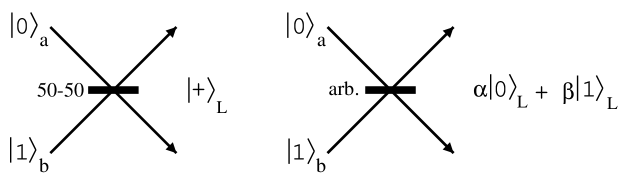
Figure 2: Diagrammatic representation of beam splitter output. By the input of a single photon in mode b and no photon in mode a, the output from a 50-50 beam splitter gives the $|+\rangle_{\mathrm{L}}$ state in the dual rail notation. Similarly by inputting single photon in mode b and no photon in mode a into an arbitrarily chosen beam splitter we have the state $\alpha|0\rangle_{\mathrm{L}}+\beta|1\rangle_{\mathrm{L}}$

[Insert figure 2 about here]

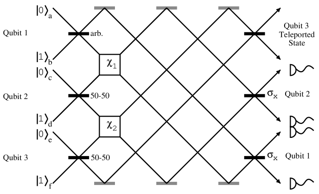
Figure 3: Optical teleportation configuration for three qubits. In this scheme we project the state of qubit one to qubit three. Qubit one’s state can initially be defined by an appropriate beam splitter denoted in the figure as an arbitrary choice. Qubits two and three are prepared in the state $|+\rangle$ via a 50-50 beam splitter. The two Kerr nonlinearities $\chi_{1}$ and $\chi_{2}$ allow the entanglement of the qubits so that the teleportation protocol can be performed. Qubits two and three are read out in the $\sigma_{x}$ basis via single photon detectors and appropriate beam splitters, this projects a state onto qubit three which is a known unitary transformation from the initial input state on qubit one.

The optical teleportation scheme is shown for three qubits in figure 3. The beam splitters on qubits two and three are 50-50 beam splitters. This ensures that the state of qubits two and three is $|+\rangle_{\mathrm{L}}$. At qubit one we have an appropriate beam splitter that will allow us to create an arbitrary state such as $\alpha|0\rangle_{\mathrm{L}}+\beta|1\rangle_{\mathrm{L}}$, this is the state we wish to teleport. Our diagrammatic representation of the beam splitters is shown in figure 2.
[Insert figure 3 about here]

To implement the Raussendorf and Briegel scheme we need to maximally entangle the state

$$|\psi\rangle_{\mathrm{L}}\otimes|+\rangle_{\mathrm{L}}\otimes|+\rangle_{\mathrm{L}}.$$ (17)

As we see from figure 3 we implement this by putting the input state

$$|1\rangle_{\mathrm{L}}=|0\rangle_{\mathrm{a}}|1\rangle_{\mathrm{b}}$$ (18)

into three beam splitters, the first one being chosen to give the state $|\psi\rangle_{\mathrm{L}}$ and the other two 50-50 beam splitters. To maximally entangle the three qubits we apply $\chi_{1}$ to mode a of qubit one and mode d of qubit two. Next we apply $\chi_{2}$ to mode c of qubit two and mode f of qubit three. Here $\chi_{1}$ and $\chi_{2}$ are of the form (16) and we write them as

$$\chi_{1} = \exp\left({i\frac{\pi}{4}(1-2a^{\dagger}a)(1-2d^{\dagger}d)}\right)$$ (19)

$$\mathrm{and}\phantom{+}\chi_{2} = \exp\left({i\frac{\pi}{4}(1-2c^{\dagger}c)(1-2f^{\dagger}f)}\right),$$ (20)

where the creation and annihilation operators $a,d,c,f,a^{\dagger},d^{\dagger},c^{\dagger}$ and $f^{\dagger}$ are the operators for the modes denoted by the same subscript a, d, c and f.

Finally the two beams which constitute each qubit are recombined for all three of the qubits and by the use of the final two beam splitters we make $\sigma_{x}$ measurements on qubits one and two (as shown in figure 3). The beam splitter on the output (qubit three) is used to rotate the final state into the initial input state $|\psi_{\mathrm{in}}\rangle$ via the feed forward information provided from the $\sigma_{x}$ measurements. As discussed in the Raussendorf and Briegel scheme this rotation is one from the set $\{1,\sigma_{x},\sigma_{z},\sigma_{x}\sigma_{z}\}$.

By analogy we shall show that this set up gives a one way quantum computer for photons. By our initial preparation of the three qubits we have the combined state of the system as

$$(\alpha|0\rangle_{\mathrm{L}}+\beta|1\rangle_{\mathrm{L}})\otimes(|0\rangle_{\mathrm{L}}+|1\rangle_{\mathrm{L}})\otimes(|0\rangle_{\mathrm{L}}+|1\rangle_{\mathrm{L}}),$$ (21)

which we can write in terms of a photon mode representation as

$$\alpha(|101010\rangle+|101001\rangle+|100110\rangle+|100101\rangle)$$

$$+\beta(|011010\rangle+|011001\rangle+|010110\rangle+|010101\rangle).$$ (22)

Here each of the six entries represent in order the mode photon number states a, b, c, d, e and f. After the operation of $\chi_{1}$ we have the state

$$\alpha(\exp\left({-i\frac{\pi}{4}}\right)|101010\rangle+\exp\left({-i\frac{\pi}{4}}\right)|101001\rangle$$

$$+\exp\left({+i\frac{\pi}{4}}\right)|100110\rangle+\exp\left({+i\frac{\pi}{4}}\right)|100101\rangle)$$

$$+\beta(\exp\left({+i\frac{\pi}{4}}\right)|011010\rangle+\exp\left({+i\frac{\pi}{4}}\right)|011001\rangle$$

$$+\exp\left({-i\frac{\pi}{4}}\right)|010110\rangle+\exp\left({-i\frac{\pi}{4}}\right)|010101\rangle),$$ (23)

by applying $\chi_{2}$ then the state of the configuration is

$$\alpha(-i|101010\rangle+|101001\rangle+i|100110\rangle+|100101\rangle)$$

$$+\beta(|011010\rangle+i|011001\rangle+|010110\rangle-i|010101\rangle).$$ (24)

After taking $\sigma_{x}$ measurements we can determine the appropriate rotation to teleport the initial state of the first qubit onto the third qubit, with the measurement-rotation relationship corresponding to that stated above. As with the Raussendorf and Briegel scheme we can readily extend this optical scheme to any arbitrary number of odd qubits, and similarly to an even number of qubits.

2.2 Optical CNOT Scheme.

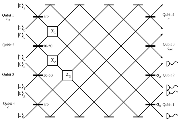
Figure 4: Optical CNOT configuration. Here qubit four and one are placed in the desired input states for the CNOT gate operation via appropriate beam splitters. Qubits two and three are put into the $|+\rangle$ superposition state. These qubits are then entangled by the three Kerr nonlinearities denoted by $\chi_{1}$, $\chi_{2}$ and $\chi_{3}$. The position of these nonlinearities play the role of entangling qubits one, three and four to qubit two. Finally $\sigma_{x}$ measurements are made on qubits one and two, projecting the $t_{\mathrm{out}}$ state to qubit three which is related to desired CNOT output by measurement dependant unitary transformations.

[Insert figure 4 about here]

The optical CNOT scheme is shown in figure 4 where corresponding to the configuration in figure 1, we have control qubit $c$ at qubit four, the $t_{\mathrm{in}}$ at qubit one and $t_{\mathrm{out}}$ at qubit three. In a similar fashion to the teleportation scheme we configure the input states using the logical state $|1\rangle_{\mathrm{L}}$ and the appropriate beam splitter (as shown in figure 2). By the use of beam splitters we set qubit one and four to give our desired inputs to the CNOT. We entangle the four qubits via the consecutive operation of $\chi_{1}$, $\chi_{2}$ and $\chi_{3}$, and make $\sigma_{x}$ measurements on qubits one and two via the final beam splitters. The final output states on qubits three and four can be rotated via the beam splitters, the actual rotation necessary is fully specified by the unitary operator (10) so that the CNOT gate works in the desired fashion.

For example if we set up the beam splitters on qubits one and four to give the initial state

$$|\psi_{\mathrm{in}}\rangle_{\mathrm{L}}=|i_{1}\rangle_{\mathrm{L}1}\otimes|+\rangle_{\mathrm{L}2}\otimes|+\rangle_{\mathrm{L}3}\otimes|i_{4}\rangle_{\mathrm{L}4},$$ (25)

then by the operation of $\chi_{1}$,$\chi_{2}$ and $\chi_{3}$ where

$$\chi_{3}=\exp\left({i\frac{\pi}{4}(1-2c^{\dagger}c)(1-2h^{\dagger}h)}\right),$$ (26)

we produce the state

$$\chi_{3}\chi_{2}\chi_{1}|\psi_{\mathrm{in}}\rangle_{\mathrm{L}} = \phantom{+}\exp\left({-i\frac{\pi}{4}((-1)^{i_{1}}+(-1)^{i_{4}}+1)}\right)|i_{1}00i_{4}\rangle_{\mathrm{L}}$$ (27)

$$+\exp\left({-i\frac{\pi}{4}((-1)^{i_{1}}+(-1)^{i_{4}}-1)}\right)|i_{1}01i_{4}\rangle_{\mathrm{L}}$$

$$+\exp\left({-i\frac{\pi}{4}((-1)^{1-i_{1}}+(-1)^{1-i_{4}}-1)}\right)|i_{1}10i_{4}\rangle_{\mathrm{L}}$$

$$+\exp\left({-i\frac{\pi}{4}((-1)^{1-i_{1}}+(-1)^{1-i_{4}}+1)}\right)|i_{1}11i_{4}\rangle_{\mathrm{L}}.$$

This corresponds to (8), and so justifies our claim that this scheme is an optical implementation of the Raussendorf and Briegel Scheme.

3 Discussion and Conclusion

The optical implementation of the scheme described here requires a Kerr nonlinearity sufficiently strong so that a single photon will give a $\pi$ phase shift, single photon sources and very efficient single photon detection. The latter two requirements, while difficult, will probably be achieved quite rapidly driven by a similar need for optical quantum key distribution [10] and the linear optics quantum computation scheme of Knill et al. [7]. Current proposals for single photon sources include exciton quantum dots [11, 12, 13], NV centres [14, 15], and surface acoustic wave devices [16]. Current proposals for detectors range from novel mesoscopic electronic devices [17], and superconducting devices [18] to novel systems that use stimulated Raman scattering [19, 20] and EIT [21]

The technology that might deliver a Kerr nonlinear device with the required strength is more difficult to identify. Recent progress in EIT schemes [22, 23, 24, 25] and cavity QED processes [26, 27] may offer some hope. It might be argued that if a Kerr nonlinearity with large single photon phase shifts was available conventional circuit based quantum computing could be achieved and there would be no need to use the measurement based scheme in this paper. We wish to emphasis the potential advantages of the scheme discussed in this paper over conventional gate network models. A gate network model based on linear optics and large Kerr nonlinearities will lead to very complicated interferometers, with complex choices of the single and two qubit conditional rotations. On the other hand the scheme described in this paper requires only a single optical layout with fixed device parameters. The actual computational algorithm that one chooses to perform is left to the measurement scenario. Thus a single nonlinear optical interferometer implementation may be used for a variety of algorithms. This may offer significant technical advantages and flexibility provided the measurements are very efficient.

On the other hand, this scheme does require fast, and highly efficient, photon number measurements, together with an ability to rapidly apply single qubit unitary operations. While these can be done with linear optics, the particular linear optics device used would need to be rapidly controlled by prior photon number measurements. As photon detection and control necessarily requires electronic signal processing, optical delay lines are likely to be needed. However there is already significant progress towards photonic quantum memories [28] that would provide a solution here, as for the similar problem in linear optical quantum computing.

We have already indicated that there is sufficient technical progress in the area of efficient single photon detection to believe that the required measurements can be achieved in the near future. There may be some advantages to trading interferometer design for complex measurement scenarios provided the required single photon detection efficiencies are available.

Measurement result	Output state
($|+\rangle_{1}$, $|+\rangle_{2}$)	$-\frac{1}{2}\exp\left({-i\frac{\pi}{4}}\right)(1+i)(|+\rangle_{1}\otimes|+\rangle_{2}\otimes(|0\rangle_{3}-|1\rangle_{3})\otimes|0\rangle_{4})$
($|+\rangle_{1}$, $|-\rangle_{2}$)	$\frac{1}{2}\exp\left({-i\frac{\pi}{4}}\right)(1-i)(|+\rangle_{1}\otimes|-\rangle_{2}\otimes(|0\rangle_{3}+|1\rangle_{3})\otimes|0\rangle_{4})$
($|-\rangle_{1}$, $|+\rangle_{2}$)	$-\frac{1}{2}\exp\left({-i\frac{\pi}{4}}\right)(1+i)(|-\rangle_{1}\otimes|+\rangle_{2}\otimes(|0\rangle_{3}-|1\rangle_{3})\otimes|0\rangle_{4})$
($|-\rangle_{1}$, $|-\rangle_{2}$)	$\frac{1}{2}\exp\left({-i\frac{\pi}{4}}\right)(1-i)(|-\rangle_{1}\otimes|-\rangle_{2}\otimes(|0\rangle_{3}+|1\rangle_{3})\otimes|0\rangle_{4})$

Table 1: Output states for four possible $\sigma_{x}$ measurements when ($|0\rangle_{1}$,$|0\rangle_{4}$) is input into the CNOT.

Measurement result	Output state
($|+\rangle_{1}$, $|+\rangle_{2}$)	$\frac{1}{2}\exp\left({-i\frac{\pi}{4}}\right)(1+i)(|+\rangle_{1}\otimes|+\rangle_{2}\otimes(|0\rangle_{3}+|1\rangle_{3})\otimes|1\rangle_{4})$
($|+\rangle_{1}$, $|-\rangle_{2}$)	$\frac{1}{2}\exp\left({-i\frac{\pi}{4}}\right)(1-i)(|+\rangle_{1}\otimes|-\rangle_{2}\otimes(|0\rangle_{3}-|1\rangle_{3})\otimes|1\rangle_{4})$
($|-\rangle_{1}$, $|+\rangle_{2}$)	$\frac{1}{2}\exp\left({-i\frac{\pi}{4}}\right)(1+i)(|-\rangle_{1}\otimes|+\rangle_{2}\otimes(|0\rangle_{3}+|1\rangle_{3})\otimes|1\rangle_{4})$
($|-\rangle_{1}$, $|-\rangle_{2}$)	$\frac{1}{2}\exp\left({-i\frac{\pi}{4}}\right)(1-i)(|-\rangle_{1}\otimes|-\rangle_{2}\otimes(|0\rangle_{3}-|1\rangle_{3})\otimes|1\rangle_{4})$

Table 2: Output states for four possible $\sigma_{x}$ measurements when ($|0\rangle_{1}$,$|1\rangle_{4}$) is input into the CNOT.

Measurement result	Output state
($|+\rangle_{1}$, $|+\rangle_{2}$)	$\frac{1}{2}\exp\left({-i\frac{\pi}{4}}\right)(1+i)(|+\rangle_{1}\otimes|+\rangle_{2}\otimes(|0\rangle_{3}+|1\rangle_{3})\otimes|0\rangle_{4})$
($|+\rangle_{1}$, $|-\rangle_{2}$)	$\frac{1}{2}\exp\left({-i\frac{\pi}{4}}\right)(1-i)(|+\rangle_{1}\otimes|-\rangle_{2}\otimes(|0\rangle_{3}-|1\rangle_{3})\otimes|0\rangle_{4})$
($|-\rangle_{1}$, $|+\rangle_{2}$)	$-\frac{1}{2}\exp\left({-i\frac{\pi}{4}}\right)(1+i)(|-\rangle_{1}\otimes|+\rangle_{2}\otimes(|0\rangle_{3}+|1\rangle_{3})\otimes|0\rangle_{4})$
($|-\rangle_{1}$, $|-\rangle_{2}$)	$-\frac{1}{2}\exp\left({-i\frac{\pi}{4}}\right)(1-i)(|-\rangle_{1}\otimes|-\rangle_{2}\otimes(|0\rangle_{3}-|1\rangle_{3})\otimes|0\rangle_{4})$

Table 3: Output states for four possible $\sigma_{x}$ measurements when ($|1\rangle_{1}$,$|0\rangle_{4}$) is input into the CNOT.

Measurement result	Output state
($|+\rangle_{1}$, $|+\rangle_{2}$)	$\frac{1}{2}\exp\left({-i\frac{\pi}{4}}\right)(1+i)(|+\rangle_{1}\otimes|+\rangle_{2}\otimes(|0\rangle_{3}-|1\rangle_{3})\otimes|1\rangle_{4})$
($|+\rangle_{1}$, $|-\rangle_{2}$)	$-\frac{1}{2}\exp\left({-i\frac{\pi}{4}}\right)(1-i)(|+\rangle_{1}\otimes|-\rangle_{2}\otimes(|0\rangle_{3}+|1\rangle_{3})\otimes|1\rangle_{4})$
($|-\rangle_{1}$, $|+\rangle_{2}$)	$-\frac{1}{2}\exp\left({-i\frac{\pi}{4}}\right)(1+i)(|-\rangle_{1}\otimes|+\rangle_{2}\otimes(|0\rangle_{3}-|1\rangle_{3})\otimes|1\rangle_{4})$
($|-\rangle_{1}$, $|-\rangle_{2}$)	$\frac{1}{2}\exp\left({-i\frac{\pi}{4}}\right)(1-i)(|-\rangle_{1}\otimes|-\rangle_{2}\otimes(|0\rangle_{3}+|1\rangle_{3})\otimes|1\rangle_{4})$

Table 4: Output states for four possible $\sigma_{x}$ measurements when ($|1\rangle_{1}$,$|1\rangle_{4}$) is input into the CNOT.

References

- [1] Raussendorf, R., and Briegel, H. J., 2001, Phys. Rev. Letts., 86, 5188.
- [2] Yamamoto, Y., Kitagawa, M., and Igeta, K., 1988, Quantum mechanical aspects of optical communication and optical computing. In Proceedings of the 3rd Asia-Pacific Physics Conference, edited by Y. W. Chan, A. F. Leung, C. N. Yang and K. Young. (Singapore: World Scientific), pp. 779-799.
- [3] Milburn, G. J., 1989, Phys. Rev. Letts., 62, 2124.
- [4] Snyder, A. W., Mitchell, D. J., Poladian, L., Rowland, D. R., and Chen, Y., 1991, J. Opt. Soc. Am. B, 8, 2102.
- [5] Mostofi, A., Malomed, B. A., and Chu, P. L., 1997, Opt. Comm., 137, 244.
- [6] Mostofi, A., Malomed, B. A., and Chu, P. L., 1998, Opt. Comm., 145, 274.
- [7] Knill, E., Laflamme, R., and Milburn, G. J., 2001, Nature (London), 409, 46.
- [8] Chefles, A., and Barnett, S. M., 1996, J. Mod. Opt., 43, 709.
- [9] Turchette, Q. A., Hood, C. J., Lange, W., Mabuchi, H., and Kimble, H. J., 1995, Phys. Rev. Letts., 75, 4710.
- [10] Gisin, N., Ribordy, G., Tittel, W., and Zbinden, H., 2002, Rev. Mod. Phys., 74, 145.
- [11] Santori, C., Pelton, M., Solomon, G., Dale, Y., and Yamamoto,Y., 2001, Phys. Rev. Letts., 86, 1502.
- [12] Michler, P., Kiraz, A., Becher, C., Schoenfeld, W. V., Petroff, P. M., Zhang, L., and Imamoglu, A., 2000, Science, 290, 2282.
- [13] Yuan, Z., Kardynal, B. E., Stevenson, R. M., Shields, A. J., Lobo, C. J., Cooper, K., Beattie, N. S., Ritchie, D. A., and Pepper, M., 2002, Science, 295, 102.
- [14] Brouri, R., Beveratos, A., Poizat, J.-Ph., and Grangier, P., 2000, Opt. Letts., 25, 1294.
- [15] Kurtseifer, C., Mayer, S., Zarda, P., and Weinfuter, H., 2000, Phys. Rev. Letts., 85, 290.
- [16] Foden, C. L., Talyanskii, V. I., Milburn, G. J., Leadbeater, M. L., and Pepper, M., 2000, Phys. Rev. A, 62, 011803(R).
- [17] Shields, A. J., O’Sullivan, M. P., Farrer, I., Ritchie, D. A., Hogg, R. A., Leadbeater, M. L., Norman, C. E., and Pepper, M., 2000, Appl. Phys. Letts., 76, 3673.
- [18] Verevkin, A., Zhang, J., Sobolewski, R., Lipatov, A., Okunev, O., Chulkova, G., Korneev, A., Smirnov, K., Gol’tsman, G. N., and Semenov, A., 2002, Appl. Phys. Letts., 80, 4687.
- [19] Imamoglu, A., 2002, Phys. Rev. Letts., 89, 163602.
- [20] James, D. F. V., and Kwiat, P. G., 2002, Phys. Rev. Letts., 89, 183601.
- [21] Munro, W. J., Nemoto, K., Beausoleil, R. G., and Spiller, T. P., 2003, quant-ph/0310066.
- [22] Fleischhauer, M., and Lukin, M. D., 2000, Phys. Rev. Letts., 84, 5094.
- [23] Petrosyan, D., and Kurizki, G., 2002, Phys. Rev. A, 65, 033833.
- [24] Paternostro, M., Kim, M. S., and Ham, B. S., 2003, Phys. Rev. A, 67, 023811.
- [25] Beausoleil, R. G., Munro, W. J., and Spiller, T. P., 2003, quant-ph/0302109.
- [26] Protsenko, I. E., Reymond, G., Schlosser, N., and Grangier, P., 2002, Phys. Rev. A, 66, 62306.
- [27] Hofmann, H. F., Kojima, K., Takeuchi. S., and Sasaki, K., 2003, J. Opt. B: Quantum Semiclass. Opt., 5, 218.
- [28] Pittman, T. B., and Franson, J.D., 2002, Phys. Rev. A, 66, 062302.