Initial correlations effects on decoherence at zero temperature

Abstract

We consider a free charged particle interacting with an electromagnetic bath at zero temperature. The dipole approximation is used to treat the bath wavelengths larger than the width of the particle wave packet. The effect of these wavelengths is described then by a linear Hamiltonian whose form is analogous to phenomenological Hamiltonians previously adopted to describe the free particle-bath interaction. We study how the time dependence of decoherence evolution is related with initial particle-bath correlations. We show that decoherence is related to the time dependent dressing of the particle. Moreover because decoherence induced by the $T=0$ bath is very rapid, we make some considerations on the conditions under which interference may be experimentally observed.

(Dated: November 15, 2005)

1 Introduction

Decoherence, that is the destruction of coherent phase relations present in the elements of the density matrix describing the system, is induced by the interaction between the quantum system and the environment. It appears to be relevant in fields ranging from quantum measurement [1] to classical-quantum interface [2], quantum information theory and computation [3] and cosmology [4]. Recently experimental evidence of environment induced decoherence has also been reported [5, 6, 7, 8, 9, 10, 11]. Several analysis of decoherence processes have been reported for the case of a particle, either free or in a potential, linearly coupled to the environment modelled as a bath of harmonic oscillators at temperature $T$ [12, 13, 14, 15, 16, 17]. Usually, initial conditions are adopted in which the system and the environment are decoupled, the interaction being effective after some initial time $t=0$ [18, 19, 20, 21]. It has been shown that, starting with factorizable initial conditions, which corresponds to the absence of initial correlations between the system and the environment, it is possible to separate the decoherence into two characteristic parts. The first, related to the thermal properties of the bath, has a typical development time which in some models goes like $T^{-1}$; the second, related to the zero point fluctuations of the oscillators of the bath, has a characteristic development time independent of temperature [22].

The time development of decoherence is also affected by the initial presence of correlations between the system and the environment [12, 13, 23, 24, 25, 26, 27]. However to choose the amount of correlations present in the initial conditions and to determine their influence on the time development may be a delicate problem mainly when interaction with the bath is always present as in the case of a charged particle interacting with the radiation field. However when the initial time is taken immediately after a fast dynamical evolution, like immediately after a collision, it appears to be reasonable to consider conditions where the particle and the bath are not in complete equilibrium [28], the extreme cases being either of completely factorized or completely correlated initial conditions. Non factorized initial conditions have in fact been adopted for particles interacting with a thermal bath corresponding to the condition where a position measurement has been made on the particle once it is in equilibrium with the bath at temperature $T$ [13, 25, 27]. Other types of initial conditions have been also considered with the particle subject to a potential abruptly modified at $t=0$ or a combination of this and of the previous ones [24]. The presence of entanglement between a particle and a bath at zero temperature has been in particular explicitly taken into account [29].

In the context of quantum computing it has been shown, that in an ensemble of two level systems interacting with a reservoir of harmonic oscillators, decoherence among the two level systems develops because of the buildup of correlations between each two level system and the environment [30]. A similar mechanism has been suggested to occur also in the case of a free charged particle interacting with the electromagnetic field vacuum. Here the decoherence among different momenta of the particle wave packet develops because of the buildup of correlations between each momentum and the associated transverse electromagnetic field structure that is responsible of the mass renormalization [31].

To treat the case of a non relativistic charged particle interacting, within the electric dipole approximation, with the electromagnetic field at temperature $T$, both the Hamiltonian approach [15] and functional techniques [13, 16] have been used. In particular development of decoherence has been studied for charged particles by examining the time dependence of the interference among two coherent wave packets.

Recently diffraction experiments have been performed where interference among different wave packets of the same particle has been observed also for rather long times [5, 6, 8, 11]. There are however indications that starting from uncoupled initial conditions decoherence develops also when the environment is at zero temperature and usually it may occur faster than the typical times of motion [14, 22]. It appears thus of interest to examine how the development of vacuum induced decoherence depends from the amount of correlation initially present between the particle and the environment.

Our model consists of a non relativistic free particle linearly interacting with a bath of harmonic oscillators at zero temperature. Our results will in particular be specialized to the case of a charged particle embedded in the electromagnetic field modes represented by a set of harmonic oscillators. This specialization is obtained from the general case by choosing the appropriate form of the coupling constants.

To study the effects of initial condition on the time development of decoherence among the momentum components of the same wave packet, the behavior of the reduced density matrix elements shall be analyzed.

2 Model

Phenomenological Hamiltonians, where the interaction is described by a linear coupling, have previously been adopted in the study of decoherence of free particles interacting with the environment treated as a bath of harmonic oscillators [12, 14, 16].

Here we consider a non relativistic free charged particle, initially moving at a velocity $\bar{\mbox{\boldmath$v$}}$, interacting with the transverse electromagnetic field.

Taking the electromagnetic field as a set of normal modes, each characterized by a wave vector $k$ and a polarization index $j$, the potential vector in the Coulomb gauge and with periodic boundary conditions taken on a volume $V$ is

$$\hat{\mbox{\boldmath$A$}}(\hat{\mbox{\boldmath$r$}})=\sum_{k,j}\mbox{\boldmath$\varepsilon$}_{k,j}\sqrt{\frac{2\pi\hbar c^{2}}{V\omega_{k}}}\left(\hat{\mathrm{a}}^{{\dagger}}_{k,j}\mathrm{e}^{-i\mbox{\boldmath$k$}\cdot\hat{\mbox{\boldmath$r$}}}+\hat{\mathrm{a}}_{k,j}\mathrm{e}^{i\mbox{\boldmath$k$}\cdot\hat{\mbox{\boldmath$r$}}}\right)\,,$$ (1)

where $\mbox{\boldmath$\varepsilon$}_{k,j}$ are the polarization vectors $(j=1,2)$, $\hat{\mbox{\boldmath$r$}}$ is the particle position operator and $\hat{\mathrm{a}}_{k,j}$ and $\hat{\mathrm{a}}^{{\dagger}}_{k,j}$ are the annihilation and creation operators of the modes that satisfy the commutation rules $[\hat{\mathrm{a}}_{k,j},\hat{\mathrm{a}}^{{\dagger}}_{k^{\prime},j^{\prime}}]=\delta_{kk^{\prime}}\delta_{jj^{\prime}}$.
The non relativistic minimal coupling Hamiltonian has the form

$$\hat{H}=\frac{1}{2m_{0}}\left[\hat{\mbox{\boldmath$p$}}-\frac{e\hat{\mbox{\boldmath$A$}}(\hat{\mbox{\boldmath$r$}})}{c}\right]^{2}+\sum_{k,j}\hbar\omega_{k}\hat{\mathrm{a}}^{{\dagger}}_{k,j}\hat{\mathrm{a}}_{k,j}\,,$$ (2)

where $\hat{\mbox{\boldmath$p$}}$ is the particle momentum operator, $m_{0}$ is the bare mass and $e$ is the charge of the particle.

In the case of a free particle the dipole approximation, typically adopted for bound charges, may be also adopted if the linear dimensions of the wave packet are small compared to the relevant wavelengths of the field. This can be applied to our Hamiltonian (2) introducing a cut off frequency $\Omega$ such that the corresponding wavelength still allows the application of dipole approximation. Moreover in order to adopt this approximation without having problems related to the distance covered in time by the particle, taking advantage of Galilean invariance of the non relativistic Hamiltonian, we put ourselves in the reference system comoving with the particle so that its average initial velocity is zero [17]. All the quantities we have introduced are obviously relative to this reference system. Within the dipole approximation, the operator $\hat{\mbox{\boldmath$r$}}$ can be replaced by a parameter $\mbox{\boldmath$r$}_{0}$ indicating the wave packet position at time $t$. In absence of interaction, in the comoving reference system, $\mbox{\boldmath$r$}_{0}$ is obviously given by the initial position of the particle. Substituting this parameter in Eq. (2), the Hamiltonian becomes

$$\hat{H}= \frac{\hat{\mbox{\boldmath$p$}}^{2}}{2m_{0}}+\sum_{k,j}\hbar\omega_{k}\hat{\mathrm{a}}^{{\dagger}}_{k,j}\hat{\mathrm{a}}_{k,j}-\frac{e}{m_{0}c}\hat{\mbox{\boldmath$p$}}\cdot\hat{\mbox{\boldmath$A$}}(\mbox{\boldmath$r$}_{0})\,,$$ (3)

where we have neglected the quadratic interaction term. In fact its physical origin is linked to the particle average kinetic energy due to the vacuum fluctuations [32], and it is usually very small compared to the linear term. On the other hand it can also be exactly eliminated by a canonical transformation of the Bogoliubov Tiablikov form [33]. This transformation has in fact been used to eliminate an analogous quadratic interaction term in the phenomenological Hamiltonian used to describe a free particle coupled to a dissipative environment [12].

The advantage of using the dipole approximation and of having a linear interaction in our system manifests itself in the fact that the Hamiltonian can be treated exactly. Moreover the Hamiltonian of Eq. (3) is formally equivalent to a model Hamiltonian previously used, in the context of quantum computing, to study the decoherence of an ensemble of two level systems coupled to a reservoir of harmonic oscillators [30]. This will permit to develop a physical analogy between these systems.

It is clear that the wave packet describing the free particle is subject to spreading. This limits the range of time where dipole approximation may be used [14]. This spreading of the wave packet has been also taken in consideration with regard to eventual problems in the definition of decoherence [34].

Using Eqs. (3) and (1) the Hamiltonian can be written as

$$\hat{H}=\sum_{p}\frac{p^{2}}{2m_{0}}\;\hat{\mbox{\boldmath$\sigma$}}_{p}+\sum_{k,j}\hbar\omega_{k}\hat{\mathrm{a}}^{{\dagger}}_{k,j}\hat{\mathrm{a}}_{k,j}+\sum_{p,k,j}\hat{\mbox{\boldmath$\sigma$}}_{p}\,g_{k,j}^{p}\left(\hat{\mathrm{a}}^{{\dagger}}_{k,j}\mathrm{e}^{-i\mbox{\boldmath$k$}\cdot\mbox{\boldmath$r$}_{0}}+\hat{\mathrm{a}}_{k,j}\mathrm{e}^{i\mbox{\boldmath$k$}\cdot\mbox{\boldmath$r$}_{0}}\right)\,,$$ (4)

where we have introduced for the momentum operator the notation $\sum_{p}\mbox{\boldmath$p$}\,\hat{\mbox{\boldmath$\sigma$}}_{p}$, with $\hat{\mbox{\boldmath$\sigma$}}_{p}=|p\rangle\langle p|$ the projection operator on the momentum eigenvalue $p$, while $g_{k,j}^{p}$ are the coupling coefficients given by

$$g_{k,j}^{p}=-\mbox{\boldmath$p$}\cdot\mbox{\boldmath$\varepsilon$}_{k,j}\frac{e}{m_{0}}\sqrt{\frac{2\pi\hbar}{V\omega_{k}}}\,.$$ (5)

Eq. (4) expresses the charge-field Hamiltonian in its unrenormalized form. To obtain the renormalized form we introduce the physical mass $m$ as

$$\frac{1}{m_{0}}=\frac{1}{m}\left(1+\frac{\delta m}{m}\right)\,,$$ (6)

where $\delta m$ represents the mass variation due to the coupling with the bath. The renormalized form is then

$$\hat{H}=\sum_{p}\frac{p^{2}}{2m}\;\hat{\mbox{\boldmath$\sigma$}}_{p}+\sum_{k,j}\hbar\omega_{k}\hat{\mathrm{a}}^{{\dagger}}_{k,j}\hat{\mathrm{a}}_{k,j}+\sum_{p,k,j}\hat{\mbox{\boldmath$\sigma$}}_{p}\,g_{k,j}^{p}\left(\hat{\mathrm{a}}^{{\dagger}}_{k,j}\mathrm{e}^{-i\mbox{\boldmath$k$}\cdot\mbox{\boldmath$r$}_{0}}+\hat{\mathrm{a}}_{k,j}\mathrm{e}^{i\mbox{\boldmath$k$}\cdot\mbox{\boldmath$r$}_{0}}\right)+\sum_{p}\frac{p^{2}}{2m}\frac{\delta m}{m}\;\hat{\mbox{\boldmath$\sigma$}}_{p}$$

The Hamiltonian under the form (4) or (2) can describe a variety of physical systems with an appropriate choice of the coefficients $g_{k,j}^{p}$. In fact a form analogous to it has been previously used, both in its unrenormalized [15, 16] and renormalized form [12, 13], with the appropriate $g_{k,j}^{p}$, to treat a particle interacting linearly with a bath.

In the following we shall keep unexplicit the expression of the coupling coefficients $g_{k,j}^{p}$, so that some results will be true not only for the charge-field interaction but in general for any particle-bath interaction with linear coupling. The explicit charge-field form (5) will be only used at the end to evidence the dependence of the results from the parameters of the system.

3 Fully correlated states

To treat the effects of the presence of particle-field correlations in the initial state, we consider at first an initial condition with the particle in complete equilibrium with the zero point field fluctuations and localized at the position $\mbox{\boldmath$r$}_{0}$. This implies that each momentum component of the wave packet is in equilibrium with the fluctuations of the electromagnetic field. The momentum of the charge commutes with the Hamiltonian (2), thus the equilibrium state of a given momentum must be an eigenstate of $\hat{H}$. In order to find these eigenstates we diagonalize exactly $\hat{H}$ by a canonical transformation using the unitary operators

$$\hat{D}_{k,j}^{p}=\exp\left[\sum_{p}\frac{\hat{\mbox{\boldmath$\sigma$}}_{p}\,g_{k,j}^{p}}{\hbar\omega_{k}}\left(\hat{\mathrm{a}}^{{\dagger}}_{k,j}\mathrm{e}^{-i\mbox{\boldmath$k$}\cdot\mbox{\boldmath$r$}_{0}}-\hat{\mathrm{a}}_{k,j}\mathrm{e}^{i\mbox{\boldmath$k$}\cdot\mbox{\boldmath$r$}_{0}}\right)\right]\,,$$ (8)

that act in the particle-field mode Hilbert space $\mathcal{H}_{S}\otimes\mathcal{H}_{F}^{k,j}$.
The action of the canonical transformation, induced by $\hat{D}_{k,j}^{p}$ on the operators $\hat{\mathrm{a}}_{k,j}$ and $\hat{\mathrm{a}}^{{\dagger}}_{k,j}$, is

$$\mathrm{\widetilde{a}}_{k,j}=\hat{D}_{k,j}^{p\,-1}\hat{\mathrm{a}}_{k,j}\hat{D}_{k,j}^{p}=\hat{\mathrm{a}}_{k,j}+\sum_{p}\frac{\hat{\mbox{\boldmath$\sigma$}}_{p}\,g_{k,j}^{p}}{\hbar\omega_{k}}\mathrm{e}^{i\mbox{\boldmath$k$}\cdot\mbox{\boldmath$r$}_{0}}\,,$$

$$\mathrm{\widetilde{a}}^{{\dagger}}_{k,j}=\hat{D}_{k,j}^{p\,-1}\hat{\mathrm{a}}^{{\dagger}}_{k,j}\hat{D}_{k,j}^{p}=\hat{\mathrm{a}}^{{\dagger}}_{k,j}+\sum_{p}\frac{\hat{\mbox{\boldmath$\sigma$}}_{p}\,g_{k,j}^{p}}{\hbar\omega_{k}}\mathrm{e}^{-i\mbox{\boldmath$k$}\cdot\mbox{\boldmath$r$}_{0}}\,.$$ (9)

To treat properly the initial condition of particle and bath when correlations are present at all frequencies, we apply the canonical transformation given in Eq. (8) to all the modes. This amounts to express $\hat{H}$ in terms of the transformed operators $\mathrm{\tilde{a}}_{k,j}$ and $\mathrm{\tilde{a}}^{{\dagger}}_{k,j}$. Thus, inverting Eq. (3) and substituting into the Hamiltonian of Eq. (2), we obtain

$$\hat{H}=\sum_{p}\frac{p^{2}}{2m}\;\hat{\mbox{\boldmath$\sigma$}}_{p}+\sum_{k,j}\hbar\omega_{k}\mathrm{\widetilde{a}}^{{\dagger}}_{k,j}\mathrm{\widetilde{a}}_{k,j}+\sum_{p}\frac{p^{2}}{2m}\frac{\delta m}{m}\;\hat{\mbox{\boldmath$\sigma$}}_{p}-\sum_{p,k,j}\frac{g_{k,j}^{p\,2}}{\hbar\omega_{k}}\;\hat{\mbox{\boldmath$\sigma$}}_{p}\,.$$ (10)

In the last term only $\hat{\mbox{\boldmath$\sigma$}}_{p}$ is an operator thus it is possible to write

$$\sum_{k,j}\frac{g_{k,j}^{p\,2}}{\hbar\omega_{k}}=\frac{p^{2}}{2m}\frac{\delta m}{m}\,,$$ (11)

by an appropriate definition of $\delta m$. In particular for the charge-electromagnetic field case, using Eq. (5) for $g_{k,j}^{p}$, taking the continuum limit, the mass variation $\delta m$ has the form

$$\delta m=\frac{4\alpha\hbar\Omega}{3\pi c^{2}}\frac{m^{2}}{m_{0}^{2}}\,,$$ (12)

where $\Omega$ is an upper frequency cut off. We see that, within second order perturbation theory in the charge, it coincides with the usual electromagnetic mass variation due to the interaction with the electromagnetic field [35].
In this way, inserting Eq. (11) in Eq. (10), the Hamiltonian reduces to

$$\hat{H}=\sum_{p}\frac{p^{2}}{2m}\;\hat{\mbox{\boldmath$\sigma$}}_{p}+\sum_{k,j}\hbar\omega_{k}\mathrm{\widetilde{a}}^{{\dagger}}_{k,j}\mathrm{\widetilde{a}}_{k,j}\,.$$ (13)

The eigenstates of $\hat{H}$ belong to the complete Hilbert space $\mathcal{H}_{S}\otimes\mathcal{H}_{F}$ and have the form $|p,\{\widetilde{n}_{k,j}\}\rangle=\prod_{k,j}\hat{D}_{k,j}^{p}|p\rangle|n_{k,j}\rangle$. In the case where each momentum is in equilibrium with the dressed vacuum state, we consider the states

$$|\widetilde{p}\rangle=|p,\{\widetilde{0}_{k,j}\}\rangle=\prod_{k,j}\hat{D}_{k,j}^{p}|p\rangle|0_{k,j}\rangle=|p\rangle\prod_{k,j}\hat{D}_{k,j}^{(p)}|0_{k,j}\rangle=|p\rangle|\{\alpha_{k,j}(p)\}\rangle\,.$$ (14)

In Eq. (14) each operator $\hat{D}_{k,j}^{(p)}$ acts only on the field-mode Hilbert space $\mathcal{H}_{F}^{k,j}$. Because of the form of $\hat{D}_{k,j}^{(p)}$, the state $|\{\alpha_{k,j}(p)\}\rangle$ indicates the product of the coherent states of all the modes of the field, each of amplitude $\alpha_{k,j}(p)=g_{k,j}^{p}\exp(-i\mbox{\boldmath$k$}\cdot\mbox{\boldmath$r$}_{0})/\hbar\omega_{k}$, associated to the component $|p\rangle$ of the wave packet in the space $\mathcal{H}_{S}$. The state $|\widetilde{p}\rangle$ represents in the electromagnetic case the state of the coupled system formed by the particle of momentum $p$ plus the transverse photons associated to it.
The action of Hamiltonian (13) on the states $|\widetilde{p}\rangle$ of Eq. (14) reduces to

$$\hat{H}|\widetilde{p}\rangle=\frac{p^{2}}{2m}|\widetilde{p}\rangle\,.$$ (15)

Thus $|\widetilde{p}\rangle$ are eigenstates of $\hat{H}$ with eigenvalues $p^{2}/2m$.
In the Schrödinger picture the time evolution operator expressed in terms of the transformed operators is

$$\hat{U}(t)=\exp\left[-\frac{i}{\hbar}\left(\sum_{p}\frac{p^{2}}{2m}\;\hat{\mbox{\boldmath$\sigma$}}_{p}+\sum_{k,j}\hbar\omega_{k}\mathrm{\widetilde{a}}^{{\dagger}}_{k,j}\mathrm{\widetilde{a}}_{k,j}\right)\,t\right]\,.$$ (16)

We consider an initial localized wave packet whose components are the correlated states of the particle in equilibrium with the bath in its vacuum state

$$|\Psi\rangle=\sum_{p}C_{p}|\widetilde{p}\rangle\,.$$ (17)

The initial density matrix of the total system is then given by

$$\widetilde{\rho}(0)=\sum_{p,p^{\prime}}C_{p}C^{*}_{p^{\prime}}|\widetilde{p}\rangle\langle\widetilde{p}^{\prime}|=\sum_{p,p^{\prime}}C_{p}C^{*}_{p^{\prime}}|p\rangle\langle p^{\prime}|\otimes|\{\widetilde{0}_{k,j}\}\rangle\langle\{\widetilde{0}_{k^{\prime},j^{\prime}}\}|\,.$$ (18)

From Eq. (18) the reduced density matrix of the particle at time $t$ is given by

$$\widetilde{\rho}_{S}(t)=\mathrm{tr}_{F}\{\hat{U}(t)\sum_{p,p^{\prime}}C_{p}C^{*}_{p^{\prime}}|p\rangle\langle p^{\prime}|\otimes|\{\widetilde{0}_{k,j}(p)\}\rangle\langle\{\widetilde{0}_{k^{\prime},j^{\prime}}(p^{\prime})\}|\hat{U}^{-1}(t)\}\,.$$ (19)

Inserting the time evolution operator (16) and the expression for $|\widetilde{p}\rangle$ (14) in Eq. (19), the matrix elements of the reduced density matrix can be cast in the form

$$\widetilde{\rho}_{S}^{p,p^{\prime}}(t)= C_{p}C^{*}_{p^{\prime}}\exp\left[{-\frac{it}{\hbar}\frac{(p^{2}-p^{\prime 2})}{2m}}\right]\mathrm{tr}_{F}\left\{|\{\alpha_{k,j}(p)\}\rangle\langle\{\alpha_{k^{\prime},j^{\prime}}(p^{\prime})\}|\right\}\,.$$

The time dependence of $\widetilde{\rho}_{S}^{p,p^{\prime}}(t)$ is given simply by $\exp\left[-it(p^{2}-p^{\prime 2})/2m\hbar\right]$, and represents the free evolution of the initial reduced matrix elements

$$\widetilde{\rho}_{S}^{p,p^{\prime}}(0)=C_{p}C^{*}_{p^{\prime}}\mathrm{tr}_{F}\left\{|\{\alpha_{k,j}(p)\}\rangle\langle\{\alpha_{k^{\prime},j^{\prime}}(p^{\prime})\}|\right\}\,.$$ (20)

It follows that for an initial state consisting of a coherent wave packet of particle-bath correlated states $|\widetilde{p}\rangle$, in the form of Eq. (18), decoherence doesn’t depend on time. The decoherence present in the reduced density matrix elements is contained in the factor $\mathrm{tr}_{F}\left\{|\{\alpha_{k,j}(p)\}\rangle\langle\{\alpha_{k^{\prime},j^{\prime}}(p^{\prime})\}|\right\}$ appearing in Eq. (20). For charge-field interaction, this factor can be interpreted as a consequence of the cloud of transverse virtual photons being associated to each momentum component of the particle.
This interpretation of the presence of decoherence in our system is analogous to the one given for the case of two level systems linearly coupled to a bath of harmonic oscillators [30], where decoherence is attributed to the buildup of correlations between the environment and the states of the two level systems.

By performing explicitly the trace on the field in the factor appearing in Eq. (20) we obtain

$$\mathrm{tr}_{F}\left\{|\{\alpha_{k,j}(p)\}\rangle\langle\{\alpha_{k^{\prime},j^{\prime}}(p^{\prime})\}|\right\} =\prod_{k^{\prime\prime},j^{\prime\prime}}\sum_{n}\langle n_{k^{\prime\prime},j^{\prime\prime}}|\prod_{k,k^{\prime},j,j^{\prime}}\hat{D}_{k,j}^{(p)}|0_{k,j}\rangle\langle 0_{k^{\prime},j^{\prime}}|\hat{D}_{k^{\prime},j^{\prime}}^{(p)-1}|n_{k^{\prime\prime},j^{\prime\prime}}\rangle$$ (21)

$$=\prod_{k,k^{\prime},j,j^{\prime}}\langle 0_{k^{\prime},j^{\prime}}|\exp\left[\frac{g_{k^{\prime},j^{\prime}}^{p^{\prime}}}{\hbar\omega_{k^{\prime}}}\left(\hat{\mathrm{a}}_{k^{\prime},j^{\prime}}\mathrm{e}^{i\mbox{\boldmath$k$}^{\prime}\cdot\mbox{\boldmath$r$}_{0}}-\hat{\mathrm{a}}^{{\dagger}}_{k^{\prime},j^{\prime}}\mathrm{e}^{-i\mbox{\boldmath$k$}^{\prime}\cdot\mbox{\boldmath$r$}_{0}}\right)\right]$$

$$\;\;\;\;\;\times\exp\left[\frac{g_{k,j}^{p}}{\hbar\omega_{k}}\left(\hat{\mathrm{a}}^{{\dagger}}_{k,j}\mathrm{e}^{-i\mbox{\boldmath$k$}\cdot\mbox{\boldmath$r$}_{0}}-\hat{\mathrm{a}}_{k,j}\mathrm{e}^{i\mbox{\boldmath$k$}\cdot\mbox{\boldmath$r$}_{0}}\right)\right]|0_{k,j}\rangle$$

$$=\prod_{k,k^{\prime},j,j^{\prime}}\langle\frac{g_{k^{\prime},j^{\prime}}^{p^{\prime}}}{\hbar\omega_{k^{\prime}}}|\frac{g_{k,j}^{p}}{\hbar\omega_{k}}\rangle\,.$$

Hence, the trace reduces to a product of coherent states. We calculate Eq. (21) explicitly in the case of a charged particle interacting with the electromagnetic field. We use the expression for the $g_{k,j}^{p}$ of Eq. (5), exploit the form of the scalar product between coherent states and perform the continuum limit of the field modes, $\sum_{k}\rightarrow\frac{V}{(2\pi c)^{3}}\int_{0}^{\infty}\mathrm{d}^{3}\omega$, to get

$$\mathrm{tr}_{F}\left\{|\{\alpha_{k,j}(p)\}\rangle\langle\{\alpha_{k^{\prime},j^{\prime}}(p^{\prime})\}|\right\}=$$

$$=\prod_{k,j}\exp\left[-\frac{\left(g_{k,j}^{p}-g_{k,j}^{p^{\prime}}\right)^{2}}{2\hbar^{2}\omega_{k}^{2}}\right]=\prod_{k,j}\exp\left\{-\frac{e^{2}}{m_{0}^{2}}\frac{2\pi\hbar}{V\omega_{k}}\frac{\left[(\mbox{\boldmath$p$}-\mbox{\boldmath$p$}\,^{\prime})\cdot\mbox{\boldmath$\varepsilon$}_{k,j}\right]^{2}}{2\hbar^{2}\omega_{k}^{2}}\right\}$$ (22)

$$=\exp\left\{-\sum_{j}\frac{e^{2}}{8\pi^{2}c^{3}m_{0}^{2}\hbar}\int_{0}^{\infty}\mathrm{d}^{3}\omega\frac{\left[(\mbox{\boldmath$p$}-\mbox{\boldmath$p$}\,^{\prime})\cdot\mbox{\boldmath$\varepsilon$}_{k,j}\right]^{2}}{\omega^{3}}\right\}=\exp\left\{-\frac{\alpha|\mbox{\boldmath$p$}-\mbox{\boldmath$p$}\,^{\prime}|^{2}}{3\pi m_{0}^{2}c^{2}}\int_{0}^{\infty}\mathrm{d}\omega\frac{\mathrm{e}^{-\omega/\Omega}}{\omega}\right\}\,,$$

where $\alpha=e^{2}/\hbar c$. The last equation has been obtained summing over the polarizations and introducing as usual a high frequency cut off factor in the integral over frequencies [16]. However the frequency integral appearing in the last equation maintains the infrared divergence. This makes the reduced density matrix of the particle diagonal and the decoherence between different momentum states of the particle is therefore complete. Thus, as a consequence of the infrared divergence, there is a super selection rule in the momenta with the emergence of stable super selection sectors [36].
However, by taking into account the finite time measurement of the particle momenta, a lower cut off frequency $\varpi$ may be introduced, the frequency $\varpi$ representing the resolution in the detection process. Introducing this lower frequency cut off $\varpi$ in Eq. (3) we obtain [37]

$$\mathrm{tr}_{F}\left\{|\{\alpha_{k,j}(p)\}\rangle\langle\{\alpha_{k^{\prime},j^{\prime}}(p^{\prime})\}|\right\} =\exp\left\{-\frac{\alpha|\mbox{\boldmath$p$}-\mbox{\boldmath$p$}\,^{\prime}|^{2}}{3\pi m_{0}^{2}c^{2}}\int_{\varpi}^{\infty}\mathrm{d}\omega\frac{\mathrm{e}^{-\omega/\Omega}}{\omega}\right\}$$

$$=\exp\left\{\frac{\alpha|\mbox{\boldmath$p$}-\mbox{\boldmath$p$}\,^{\prime}|^{2}}{3\pi m_{0}^{2}c^{2}}\left[\gamma+\ln\frac{\varpi}{\Omega}+\sum_{n=1}^{\infty}\frac{(-1)^{n}}{n\,n!}\,\left(\frac{\varpi}{\Omega}\right)^{n}\right]\right\}\,,$$

where $\gamma=0.577216$ is the Euler’s constant.
For $\varpi/\Omega\ll 1$ Eq. (3) can be approximated as

$$\mathrm{tr}_{F}\left\{|\{\alpha_{k,j}(p)\}\rangle\langle\{\alpha_{k^{\prime},j^{\prime}}(p^{\prime})\}|\right\}=\exp\left\{\frac{\alpha|\mbox{\boldmath$p$}-\mbox{\boldmath$p$}\,^{\prime}|^{2}}{3\pi m_{0}^{2}c^{2}}\ln\frac{\varpi}{\Omega}\right\}\,,$$ (24)

and the initial reduced density matrix elements of Eq. (20) take the form

$$\widetilde{\rho}_{S}^{p,p^{\prime}}(0)=C_{p}C^{*}_{p^{\prime}}\exp\left\{\frac{\alpha|\mbox{\boldmath$p$}-\mbox{\boldmath$p$}\,^{\prime}|^{2}}{3\pi m_{0}^{2}c^{2}}\ln\frac{\varpi}{\Omega}\right\}\,.$$ (25)

Now decoherence between momenta in the matrix elements of Eq. (25) is not complete anymore and depends both on the distance between the values of the particle momenta and on $\varpi$.

4 Partially correlated states

The need of introducing a lower cut off frequency can also derive from the initial packet preparation rather than from the final measurement. If the initial packet is localized by a measurement with an uncertainty $\Delta x$ and then with a momentum uncertainty $\Delta p\sim\hbar/\Delta x$, this is equivalent to a minimum measurement time $\Delta t\sim\hbar/\Delta p\Delta v$ [22, 38], to which it is possible to associate a lower frequency limit $\varpi\sim 1/\Delta t$ to modes that have reached equilibrium with the particle.
This indicates that we can start from an initial condition with the particle in equilibrium only with the modes at a frequency $\omega>\varpi$ while it has no correlation with those at $\omega<\varpi$. Thus we take as initial condition a state whose momentum components have the form

$$|\tilde{p}_{\varpi}\rangle=|p\rangle\prod_{j}\prod_{k=0}^{\varpi/c}|0_{k,j}\rangle\prod_{\bar{k}=\varpi/c}^{\infty}|\tilde{0}_{\bar{k},j}\rangle\;.$$ (26)

From Eq. (26) we build the initial wave packet $\sum_{p}C_{p}|\tilde{p}_{\varpi}\rangle$ that corresponds to the initial density matrix

$$\tilde{\rho}_{\varpi}(0)=\sum_{p,p^{\prime}}C_{p}C^{*}_{p^{\prime}}|p\rangle\langle p^{\prime}|\prod_{j}\prod_{k=0}^{\varpi/c}|0_{k,j}\rangle\langle 0_{k,j}|\prod_{\bar{k}=\varpi/c}^{\infty}|{\tilde{0}}_{\bar{k},j}\rangle\langle\tilde{0}_{\bar{k},j}|\;.$$ (27)

In Eq. (27) the modes at frequency higher than $\varpi$ are distinguished from those at lower frequency and we have eliminated the cross terms between the two mode regions. In fact these terms won’t contribute to the reduced density matrix elements because they will be eliminated in the field trace and then we don’t consider them.

To discuss the time evolution from the initial state represented by the density matrix $\tilde{\rho}_{\varpi}(0)$ it is useful to separate in the Hamiltonian of Eq. (2) the parts at frequency larger and smaller than $\varpi$, i.e.

$$\hat{H} =\sum_{p}\frac{p^{2}}{2m}\;\hat{\mbox{\boldmath$\sigma$}}_{p}+\hat{H}_{\omega<\varpi}+\hat{H}_{\omega>\varpi}+\sum_{p}\frac{p^{2}}{2m}\frac{\delta m}{m}\;\hat{\mbox{\boldmath$\sigma$}}_{p}$$

$$=\sum_{p}\frac{p^{2}}{2m}\;\hat{\mbox{\boldmath$\sigma$}}_{p}+\left[\sum_{j,k=0}^{\varpi/c}\hbar\omega_{k}\hat{\mathrm{a}}^{{\dagger}}_{k,j}\hat{\mathrm{a}}_{k,j}+\sum_{p,j,k=0}^{\varpi/c}\hat{\mbox{\boldmath$\sigma$}}_{p}\,g_{k,j}^{p}\left(\hat{\mathrm{a}}^{{\dagger}}_{k,j}\mathrm{e}^{-i\mbox{\boldmath$k$}\cdot\mbox{\boldmath$r$}_{0}}+\hat{\mathrm{a}}_{k,j}\mathrm{e}^{i\mbox{\boldmath$k$}\cdot\mbox{\boldmath$r$}_{0}}\right)\right]$$

$$+\left[\sum_{j,k=\varpi/c}^{\infty}\hbar\omega_{k}\hat{\mathrm{a}}^{{\dagger}}_{k,j}\hat{\mathrm{a}}_{k,j}+\sum_{p,j,k=\varpi/c}^{\infty}\hat{\mbox{\boldmath$\sigma$}}_{p}\,g_{k,j}^{p}\left(\hat{\mathrm{a}}^{{\dagger}}_{k,j}\mathrm{e}^{-i\mbox{\boldmath$k$}\cdot\mbox{\boldmath$r$}_{0}}+\hat{\mathrm{a}}_{k,j}\mathrm{e}^{i\mbox{\boldmath$k$}\cdot\mbox{\boldmath$r$}_{0}}\right)\right]+\sum_{p}\frac{p^{2}}{2m}\frac{\delta m}{m}\;\hat{\mbox{\boldmath$\sigma$}}_{p}\;.$$

To treat properly the presence in the initial condition of correlations with the high frequency modes, in $\hat{H}$, we apply the canonical transformation (8) only to the modes at frequency higher than $\varpi$. This amounts to express only $\hat{H}_{\omega>\varpi}$ in terms of the transformed operators $\mathrm{\tilde{a}}_{k,j}$ and $\mathrm{\tilde{a}}^{{\dagger}}_{k,j}$. Following the same steps leading from Eq. (2) to Eq. (10) we get

$$\hat{H}=\sum_{p}\frac{p^{2}}{2m}\;\hat{\mbox{\boldmath$\sigma$}}_{p}+\hat{H}_{\omega<\varpi}+\sum_{j,k=\varpi/c}^{\infty}\hbar\omega_{k}\mathrm{\tilde{a}}^{{\dagger}}_{k,j}\mathrm{\tilde{a}}_{k,j}+\sum_{p}\frac{p^{2}}{2m}\frac{\delta m}{m}\;\hat{\mbox{\boldmath$\sigma$}}_{p}-\sum_{p,j,k=\varpi/c}^{\infty}\frac{g_{k,j}^{p\,2}}{\hbar\omega_{k}}\hat{\mbox{\boldmath$\sigma$}}_{p}\,.$$ (29)

In the last term of Eq. (29) only $\hat{\mbox{\boldmath$\sigma$}}_{p}$ is an operator and, in analogy to Eq. (11), it is possible to write by an appropriate definition of $\delta m_{>\varpi}$

$$\sum_{j,k=\varpi/c}^{\infty}\frac{g_{k,j}^{p\,2}}{\hbar\omega_{k}}=\frac{p^{2}}{2m}\frac{\delta m_{>\varpi}}{m}\,.$$ (30)

$\delta m_{>\varpi}$ corresponds to the mass variation of the particle due to dressing with the high frequency modes. Thus, for the sum of the last two terms present in Eq. (29) we obtain

$$\sum_{p}\frac{p^{2}}{2m}\frac{\delta m}{m}\;\hat{\mbox{\boldmath$\sigma$}}_{p}-\sum_{p,j,k=\varpi/c}^{\infty}\frac{g_{k,j}^{p\,2}}{\hbar\omega_{k}}\;\hat{\mbox{\boldmath$\sigma$}}_{p}=\sum_{p}\frac{p^{2}}{2m}\frac{\delta m_{<\varpi}}{m}\;\hat{\mbox{\boldmath$\sigma$}}_{p}\;,$$ (31)

where $\delta m_{<\varpi}=\delta m-\delta m_{>\varpi}$ indicates the mass variation of the particle due to dressing with the low frequency modes. Using Eq. (31) in Eq. (29), the Hamiltonian $\hat{H}$ becomes

$$\hat{H}=\sum_{p}\frac{p^{2}}{2m}\;\hat{\mbox{\boldmath$\sigma$}}_{p}+\sum_{p}\frac{p^{2}}{2m}\frac{\delta m_{<\varpi}}{m}\;\hat{\mbox{\boldmath$\sigma$}}_{p}+\hat{H}_{\omega<\varpi}+\tilde{H}_{\omega>\varpi}=\sum_{p}\frac{p^{2}}{2m_{\varpi}}\,\hat{\mbox{\boldmath$\sigma$}}_{p}+\hat{H}_{\omega<\varpi}+\tilde{H}_{\omega>\varpi}\;,$$ (32)

where $\tilde{H}_{\omega>\varpi}=\sum_{j,k=\varpi/c}^{\infty}\hbar\omega_{k}\mathrm{\tilde{a}}^{{\dagger}}_{k,j}\mathrm{\tilde{a}}_{k,j}$ and the mass $m_{\varpi}$ is defined by

$$\frac{1}{m_{\varpi}}=\frac{1}{m}\left(1+\frac{\delta m_{<\varpi}}{m}\right)\,.$$ (33)

No renormalization term is present in the Hamiltonian of Eq. (32). This is due to the fact that only the interaction with modes at frequency $\omega<\varpi$ appears in $H$ and that the mass $m_{\varpi}$ represents the bare mass with respect to the low frequency modes. The Hamiltonian being now expressed in terms of the bare mass, the low frequency renormalization term disappears.

In the Hamiltonian $\hat{H}$ (32) the terms $\sum_{p}(p^{2}/2m_{\varpi})\,\hat{\mbox{\boldmath$\sigma$}}_{p}$, $\hat{H}_{\omega<\varpi}$ and $\tilde{H}_{\omega>\varpi}$ commute among them. This allows to analyze in a transparent way the influence of each of these terms on the time evolution of the reduced density matrix elements of $\tilde{\rho}_{\varpi}(0)$ and to discuss separately the effects of high frequency correlated and low frequency uncorrelated modes. In fact we can write the reduced density matrix elements of the particle at time $t$ as

$$\tilde{\rho}_{S\,\varpi}^{p,p^{\prime}}(t)=\langle p|\mathrm{tr}_{F}\{\hat{U}_{\varpi}(t)\tilde{\rho}_{\varpi}(0)\hat{U}_{\varpi}^{-1}(t)\}|p^{\prime}\rangle\;,$$ (34)

where $\hat{U}_{\varpi}(t)$ is the time evolution operator, that may be written as the product of three operators $\hat{U}_{\varpi}(t)=\hat{U}_{S,\varpi}(t)\hat{U}_{\omega<\varpi}(t)\tilde{U}_{\omega>\varpi}(t)$. The first, $\hat{U}_{S,\varpi}=\exp\left[-i\sum_{p}(p^{2}/2m_{\varpi}\hbar)\hat{\mbox{\boldmath$\sigma$}}_{p}\,t\right]$, depends on the kinetic energy and can be shown to affect only the free evolution of reduced density matrix elements. Introducing the time-ordering operator $T_{\leftarrow}$, the second term is $\hat{U}_{\omega<\varpi}(t)=\mathrm{T}_{\leftarrow}\exp\left[-i\int_{0}^{t}\mathrm{d}s\hat{H}_{\omega<\varpi}(s)/\hbar\right]$, and depends on the modes at frequency lower than $\varpi$, while the third term is $\tilde{U}_{\omega>\varpi}(t)=\mathrm{T}_{\leftarrow}\exp\left[-i\int_{0}^{t}\mathrm{d}s\tilde{H}_{\omega>\varpi}(s)/\hbar\right]$ and depends on those at frequency higher than $\varpi$. Thus, Eq. (34) can be written as

$$\tilde{\rho}_{S\,\varpi}^{p,p^{\prime}}(t)=\exp\left[-\frac{it}{\hbar}\frac{(p^{2}-p^{\prime 2})}{2m_{\varpi}}\right]\langle p|\mathrm{tr}_{F}\{\hat{U}_{\omega<\varpi}(t)\left[\tilde{U}_{\omega>\varpi}(t)\tilde{\rho}_{\varpi}(0)\tilde{U}_{\omega>\varpi}^{-1}(t)\right]\hat{U}_{\omega<\varpi}^{-1}(t)\}|p^{\prime}\rangle\;.$$ (35)

$\hat{U}_{\omega<\varpi}$ acts only on the low frequency part of the density operator $\tilde{\rho}_{\varpi}(0)$ of Eq. (27) representing the modes uncorrelated to the particle momenta. This leads to a time evolution of this part of $\tilde{\rho}_{\varpi}(0)$ formally identical to the one we would get from a fully uncorrelated initial condition.

For a charge interacting with the electromagnetic field we may directly use, for the evolution of the low frequency part of $\tilde{\rho}_{\varpi}(t)$, the results already obtained in [31], that is:

$$\rho_{S}^{p,p^{\prime}}(t)=\rho_{S}^{p,p^{\prime}}(0)\exp\left[-\frac{it}{\hbar}\frac{(p^{2}-p^{\prime 2})}{2m_{0}}\right]\exp{\Gamma^{p,p^{\prime}}(t)}\;,$$ (36)

where the complex decoherence function $\Gamma^{p,p^{\prime}}(t)=\Gamma^{p,p^{\prime}}_{r}(t)+i\Gamma^{p,p^{\prime}}_{i}(t)$ has been introduced with $\Gamma^{p,p^{\prime}}_{r}(t)$ and $\Gamma^{p,p^{\prime}}_{i}(t)$ given respectively by the integral expressions

$$\Gamma^{p,p^{\prime}}_{r}(t)=-\frac{2\alpha}{3\pi}\frac{|\mbox{\boldmath$p$}-\mbox{\boldmath$p$}\,^{\prime}|^{2}}{m_{0}^{2}c^{2}}\int_{0}^{\infty}\mathrm{d}\omega\exp\left(-\frac{\omega}{\Omega}\right)\frac{(1-\cos\omega t)}{\omega}\;,$$ (37)

which corresponds to the expression of $\Gamma^{p,p^{\prime}}_{r}(t)$ given in [31] in the limit $T=0$, in which only the vacuum contribution remains so that $\Gamma^{p,p^{\prime}}_{r}(t)=\Gamma^{p,p^{\prime}}_{vac}(t)$, and

$$\Gamma^{p,p^{\prime}}_{i}(t) =\frac{2e^{2}\left(p^{2}-p^{\prime 2}\right)}{3\pi\hbar m_{0}^{2}c^{3}}\int_{0}^{\infty}\mathrm{d}\omega\exp\left(-\frac{\omega}{\Omega}\right)\left(t-\frac{\sin\omega t}{\omega}\right).$$ (38)

Here, because of Eq. (27), in the integrals defining $\Gamma^{p,p^{\prime}}_{i}(t)$ and $\Gamma^{p,p^{\prime}}_{r}(t)$ we replace the cut off factor $\exp\left(-\omega/\Omega\right)$ with the step function $\Theta(\varpi-\omega)$. In such a way we obtain a new expression for the real and imaginary part of the decoherence function, $\bar{\Gamma}^{p,p^{\prime}}_{vac}(t)$ and $\bar{\Gamma}^{p,p^{\prime}}_{i}(t)$, which will depend only on the modes at frequency lower than $\varpi$ as:

$$\bar{\Gamma}^{p,p^{\prime}}_{vac}(t) =-\frac{2\alpha}{3\pi}\frac{|\mbox{\boldmath$p$}-\mbox{\boldmath$p$}\,^{\prime}|^{2}}{m_{0}^{2}c^{2}}\int_{0}^{\infty}\mathrm{d}\omega\frac{(1-\cos\omega t)}{\omega}\Theta(\varpi-\omega)$$ (39)

$$=-\frac{2\alpha}{3\pi}\frac{|\mbox{\boldmath$p$}-\mbox{\boldmath$p$}\,^{\prime}|^{2}}{m_{0}^{2}c^{2}}\left[\gamma-\mathrm{Ci}(\varpi t)+\ln\varpi t\right]\;,$$

$$\bar{\Gamma}^{p,p^{\prime}}_{i}(t) =\frac{2e^{2}\left(p^{2}-p^{\prime 2}\right)}{3\pi\hbar m_{0}^{2}c^{3}}\int_{0}^{\infty}\mathrm{d}\omega\left(t-\frac{\sin\omega t}{\omega}\right)\Theta(\varpi-\omega)=\frac{2\alpha}{3\pi}\frac{p^{2}-p^{\prime 2}}{m_{0}^{2}c^{2}}[\varpi t-\mathrm{Si}(\varpi t)]\;,$$ (40)

where $\mathrm{Ci}(\varpi t)$ and $\mathrm{Si}(\varpi t)$ are the cosine and sine integral function [37].
Using the expression of $\mathrm{Ci}(\varpi t)$ for small and large values of $\varpi t$ [37] we obtain for $\bar{\Gamma}^{p,p^{\prime}}_{vac}(t)$

$$\bar{\Gamma}^{p,p^{\prime}}_{vac}(t)\>\approx\>\cases{-\frac{2\alpha}{3\pi}\frac{|\mbox{\boldmath$p$}-\mbox{\boldmath$p$}\,^{\prime}|^{2}}{m_{0}^{2}c^{2}}\frac{\varpi^{2}t^{2}}{4}&for $\varpi t\ll 1$\\ -\frac{2\alpha}{3\pi}\frac{|\mbox{\boldmath$p$}-\mbox{\boldmath$p$}\,^{\prime}|^{2}}{m_{0}^{2}c^{2}}\ln\varpi t&for $\varpi t\gg 1$\\ }$$ (41)

Eq. (41) shows that there are a quadratic and a logarithmic time evolution regimes. The transition from the first to the second one occurs at a typical time $\tilde{t}\approx\varpi^{-1}$ with $|\bar{\Gamma}^{p,p^{\prime}}_{vac}(\tilde{t})|=Q\approx\frac{2\alpha}{3\pi}\frac{|\mbox{\boldmath$p$}-\mbox{\boldmath$p$}\,^{\prime}|^{2}}{m_{0}^{2}c^{2}}$. The effective magnitude of $\bar{\Gamma}^{p,p^{\prime}}_{vac}(t)$ at a given time depends both on $\varpi$, which is determined by the preparation or observation procedure, and on $Q$ which depends on the charge and the mass of the particle and on the distance of the reduced density matrix element from the diagonal in the momentum space. The vacuum influence on the time evolution of decoherence for $Q\ll 1$ remains small because of the logarithmic dependence of $\bar{\Gamma}^{p,p^{\prime}}_{vac}(t)$ from time. Its effect increases with $Q$ and for sufficiently large $Q$ decoherence may become effective at times $t\geq\varpi^{-1}$. This behavior is shown in figure 1.

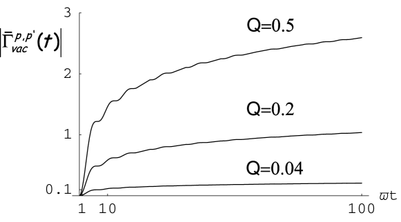
Figure 1: Time dependence of $|\bar{\Gamma}^{p,p^{\prime}}_{vac}(t)|$ for different values of the parameter $Q$.

In conclusion we see that the effect of the low frequency modes, described by $U_{\omega<\varpi}(t)$, reduces to a multiplication factor in the reduced density matrix element $\tilde{\rho}_{S\,\varpi}^{p,p^{\prime}}(t)$ of the form $\exp\left[{\bar{\Gamma}^{p,p^{\prime}}_{vac}(t)+i\bar{\Gamma}^{p,p^{\prime}}_{i}(t)}\right]$ where $\bar{\Gamma}^{p,p^{\prime}}_{vac}(t)$ is given by Eq. (39) and $\bar{\Gamma}^{p,p^{\prime}}_{i}(t)$ by Eq. (40).

With regards to the third term in the Hamiltonian (32), $\tilde{H}_{\omega>\varpi}$, representing the high frequency modes contribution, its action on the time evolution of $\tilde{\rho}_{S\,\varpi}^{p,p^{\prime}}(t)$ can be obtained by following the equations that from Eq. (16) lead to Eq. (25), where the lower frequency represents in that case the effect of the finite resolution of the detection process. We are therefore led to a term formally identical with the one of Eq. (25) that doesn’t influence the low frequency part of $\tilde{\rho}_{\varpi}(0)$.

Joining together all the previous considerations we finally obtain for the complete expression of the reduced density matrix elements

$$\tilde{\rho}_{S\,\varpi}^{p,p^{\prime}}(t)= C_{p}C^{*}_{p^{\prime}}\exp\left[-\frac{it}{\hbar}\frac{(p^{2}-p^{\prime 2})}{2m_{\varpi}}\right]\exp\left[i\frac{2\alpha\left(\varpi t-\mathrm{Si}(\varpi t)\right)}{3\pi m_{0}^{2}c^{2}}(p^{2}-p^{\prime 2})\right]$$ (42)

$$\left.\times\exp\left\{-\frac{2\,\alpha\,|\mbox{\boldmath$p$}-\mbox{\boldmath$p$}\,^{\prime}|^{2}}{3\pi m_{0}^{2}c^{2}}\left[\gamma-\mathrm{Ci}(\varpi t)+\ln\varpi t\right]\right\}\right.\exp\left[\frac{\alpha|\mbox{\boldmath$p$}-\mbox{\boldmath$p$}\,^{\prime}|^{2}}{3\pi m_{0}^{2}c^{2}}\ln\frac{\varpi}{\Omega}\right]\;.$$

We observe that with regard to the contribution in Eq. (42) of the low frequency modes, we have used Eqs. (39) and (40) whose form is valid at all the times. For the contribution of the high frequency modes we have used Eq. (25) which is valid in the limit $\varpi/\Omega\ll 1$. However it is possible from Eq. (42) to obtain a simplified form of $\tilde{\rho}_{S\,\varpi}^{p,p^{\prime}}(t)$ for small and large $\varpi t$, using for $\bar{\Gamma}^{p,p^{\prime}}_{vac}(t)$ the corresponding expressions of Eq. (41).

The form given by Eq. (42) describes the time evolution of the reduced density matrix elements when, in the initial state, correlations with the field modes at frequency larger than $\varpi$ are present. The form for $\tilde{\rho}_{S\,\varpi}^{p,p^{\prime}}(t)$ of Eq. (42) is intermediate between the two extreme forms, completely correlated (3, 3) and uncorrelated (36), and it coincides with them respectively in the limits $\varpi\rightarrow 0$ and $\varpi\rightarrow\Omega$.

One must observe that in the fully correlated case ($\varpi=0$) the particle is completely entangled with the field and the initial reduced density matrix (18) contains already all the decoherence, which therefore remains constant with time. For $\varpi\neq 0$ the initial entanglement is partial and it is the coupling dynamics that induces the progressive entanglement with the modes at frequency less than $\varpi$ thus leading to an increase of the decoherence present at $t=0$.

5 Summary and Conclusions

We have studied the decoherence among the momentum components of a free particle wave packet linearly interacting with a zero temperature bath by working out the time dependence of the off diagonal elements of the reduced density matrix of the particle. We have also examined the influence on the decoherence development by the initial conditions and in particular by the presence of correlations between the particle and the environment.

The influence of initial conditions on decoherence has been previously studied by examining the attenuation of coherence between a pair of coherent wave packets in the case of a particle interacting with a bath either at finite [27] or zero temperature [29].

We have considered initial conditions ranging from the case of absence of initial correlations to the case where they are fully developed. The particle-bath system is described in the former case by a factorized density matrix and in the latter, which corresponds to a stationary condition, by a linear combination of the eigenstates of the total Hamiltonian. The reason to consider this range of initial conditions is linked to the fact that when the interaction between the system and the bath is always present, as in the case of a charged particle interacting with the radiation field, it isn’t appropriate to start from a condition where no correlations are present. On the other hand because of either a finite measurement time or preparation time it is not appropriate to start from a condition where there is complete equilibrium among the particle momenta and all the field modes. By taking for example a finite preparation time $\tau$, one is led to consider a situation where equilibrium correlations have been established only with the modes at frequency higher than $\varpi\approx 1/\tau$, while modes of lower frequency are uncorrelated.

This intermediate initial situation may be described by a density matrix formed by two parts: the first, time independent, describes the initial correlations already established with modes at frequency higher than $\varpi$; the second time dependent, will describe the establishing of correlations with the modes at frequency lower than $\varpi$. We have shown that, for the case of linear interaction, the increase of decoherence is at first rapid and goes like $t^{2}$ while, after a transition time of the order of $\varpi^{-1}$, slows and goes as $\ln t$, in a certain sense reaching a plateau at $t\approx\varpi^{-1}$. The effect of partially correlated initial conditions does show only in the transition time, while the value that decoherence reaches at the transition time is only a function of the physical parameters of the particle like the value of the coupling constant, the particle mass and the distance of the matrix element from the diagonal.

We have explicitly obtained our results for the case of a charged particle interacting with the electromagnetic field. In fact, by an appropriate choice of the width of the particle wave packet we have shown that it is possible to adopt the dipole approximation. In this context and by considering the case of low field intensities, we have shown that the interaction Hamiltonian becomes linear. In this case then the value of the decoherence at the transition time $\varpi^{-1}$ depends from the combination of parameters given by $Q\approx\frac{2\alpha}{3\pi}\frac{|\mbox{\boldmath$p$}-\mbox{\boldmath$p$}\,^{\prime}|^{2}}{m_{0}^{2}c^{2}}$. Moreover the time independent part of the reduced density matrix $\tilde{\rho}_{\varpi}(0)$ given by Eq. (27) presents an infrared divergence when the preparation time is large and thus $\varpi\rightarrow 0$ (25). In this case the decoherence in momentum space is complete and the divergence is connected with the establishing of a complete correlation with the low frequency modes. For finite $\varpi$, with the buildup in time of correlations with the low frequency modes these become populated. This process gives rise to a cloud of photons around the particle which are then responsible of mass renormalization. The two phenomena of decoherence due to zero point modes and dressing of the particle are thus related. Moreover when one performs an experiment that takes a finite time, that shows the presence of decoherence, like in interference experiments [6, 11], it is appropriate to ask the form of the reduced density matrix that correctly describes the experiment. From what said previously it appears that the trace must be performed only on those field modes where supposedly equilibrium hasn’t been reached. Then the characteristic time in which decoherence becomes complete is a factor $\Omega/\varpi$ larger than the characteristic decoherence time one obtains starting from completely uncorrelated initial condition [31].

Our analysis has been conducted in the context of non relativistic QED which is an effective low energy theory with the cut off frequency $\Omega$, in the spirit of modern quantum field theory, parameterizing the physics due to the higher frequencies [39]. For this reason our final results must show a dependence on $\Omega$, that is however as usual weak (logarithmic), as for example in the case of non relativistic expression for the Lamb shift. The appearance of the bare mass $m_{0}$ in our results, e.g. in Eq. (20) and (42), is due to its use in the definition of the coupling coefficients $g_{k,j}^{p}$ (5). The $g_{k,j}^{p}$ in Eq. (2) and (4) could be expressed in terms of the fully and partially dressed mass by introducing a further renormalization term which is however $O(e^{3})$ and therefore typically neglected. This procedure would eventually lead to final reduced density matrix expressions given in terms of the dressed masses with a correction in the exponents of $O(e^{4})$ with respect to the actually results. This may be alternatively seen by expressing, directly in the final expressions for decoherence, the bare mass in terms of the dressed masses obtaining a further term containing the product of the mass variation of $O(e^{2})$ for a factor $\alpha$.

As a final consideration we observe that a state describing an electron not in complete equilibrium with its surrounding field was suggested by Feinberg [40] to represent the electron immediately after a scattering event of duration $\tau$. In fact, due to causality requirements the electron can reach equilibrium only with its field within a region of size $l\leq c\tau$. Similar states of incomplete equilibrium have been also studied in QED when rapid changes occur in atomic or molecular sources [28]. However the most promising field where states of not complete equilibrium may be implemented is solid state physics. The use of ultra fast spectroscopic techniques has in fact permitted the generation of almost bare electron-hole states and to follow the time evolution of the dressing process due to the interaction with the phonon field [41]. Taking into account the previous considerations, one can envisage a process where, starting from states of not complete equilibrium, the evolution of decoherence gives rise, in principle, to observable effects. Let’s in fact consider the scattering of a charged particle from two scattering centers, the process lasting a finite time $\tau\approx\varpi^{-1}$. From the considerations developed in this paper one must expect that, after the scattering, the state of the particle may be described by Eq. (27) and the decoherence which develops after the scattering gives rise to a decrease of the interference effects which depends on $\varpi$.

References

References

- [1] Joos E, Zeh H D, Kiefer C, Giulini D, Kupsch J and Stamatescu I O 2002 Decoherence and the Appearance of a Classical World in Quantum Theory (Springer, New York, sec. ed.)
- [2] Zurek W H 2003 Rev. Mod. Phys.75 715
- [3] Unruh W G 1995 Phys. Rev.A 51 992
- [4] Barvinsky A O, Kamenshchik A Y, Kiefer C and Mishakov I V 1999 Nucl. Phys.B 551 374
- [5] Brune M, Hagley E, Dreyer J, Ma tre X, Maali A, Wunderlich C, Raimond J M and Haroche S 1996 Phys. Rev. Lett.77 4887
- [6] Myatt C J, King B E, Turchette Q A, Sackett C A, Klelpinski D, Itano W M, Monroe C and Wineland D J 2000 Nature 403 269
- [7] Raimond J M, Brune M and Haroche S 2001 Rev. Mod. Phys.73 565
- [8] Brezger B, Hackerm ller L, Uttenthaler S, Petschinka J, Arndt M, and Zeilinger A 2002 Phys. Rev. Lett.88 100404
- [9] Hornberger K, Uttenthaler S, Brezger B, Hackerm ller L, Arndt M and Zeilinger A 2003 Phys. Rev. Lett.90 160401
- [10] Auffeves A, Maioli P, Meunier T, Gleyzes S, Nogues G, Brune M, Raimond J M and Haroche S 2003 Phys. Rev. Lett.91 230405
- [11] Hackerm ller L, Hornberger K, Brezger B, Zeilinger A and Arndt M 2004 Nature 427 711
- [12] Hakim V and Ambegaokar V 1985 Phys. Rev.A 32 423
- [13] Barone P M V B and Caldeira A O 1991 Phys. Rev.A 43 57
- [14] Ford L H 1993 Phys. Rev.D 47 5571
- [15] Dürr D and Spohn H 2000 in: Decoherence: theoretical, experimental, and conceptual problems, edited by Ph. Blanchard, D. Giulini, E. Joos, C. Kiefer and I. O. Stamatescu, Lecture Notes in Physics 538 77 (SpringerVerlag, Berlin)
- [16] Breuer H P and Petruccione F 2001 Phys. Rev.A 63 032102
- [17] Mazzitelli F D, Paz J P and Villanueva A 2003 Phys. Rev.A 68 062106
- [18] Feynman R P and Vernon F L 1963 Ann. Phys., NY24 118
- [19] Caldeira A O and Leggett A J 1985 Phys. Rev.A 31 1059
- [20] Mozyrsky D and Privman V 1998 J. Stat. Phys. 91 787
- [21] Tolkunov D and Privman V 2004 Phys. Rev.A 69 062309
- [22] Breuer H P and Petruccione F 2002 The Theory of Open Quantum Systems (Oxford University)
- [23] Grabert H, Schramm P and Ingold G L 1988 Phys. Rep. 168 115
- [24] Smith C M and Caldeira A O 1990 Phys. Rev.A 41 3103
- [25] Romero L D and Paz J P 1997 Phys. Rev.A 55 4070
- [26] Ford G W, Lewis J T and O’Connell R F 2001 Phys. Rev.A 64 032101
- [27] Lutz E 2003 Phys. Rev.A 67 022109
- [28] Compagno G, Passante R and Persico F 1995 Atom-Field Interactions and Dressed Atoms (Cambridge University Press)
- [29] Ford G W and O’Connell R F 2003 J. Opt. B: Quantum Semiclass. Opt.5 S609
- [30] Palma G M, Suominen K A and Ekert A K 1996 Proc. R. Soc. Lond. A452 567
- [31] Bellomo B, Compagno G and Petruccione F 2004 Proceedings of Quantum Communication, Measurement and Computing (QCMC04), AIP Conference Proceedings, 734, 413 Issue 1
- [32] Weisskopf V F 1939 Phys. Rev.56 72
- [33] Tiablikov S V 1967 Methods in the Quantum Theory of Magnetism (Plenum Press, New York)
- [34] O’Connell R F 2005 arXive:quant-ph/0501097
- [35] Sakurai J K 1977 Advanced quantum mechanics (Addison-Wesley)
- [36] Kupsch J 2002 Pramana J. Phys. 59 195
- [37] Abramowitz M and Stegun I A 1972 Handbook of mathematical functions (Dover)
- [38] Wheeler J A and Zurek W H 1983 Quantum theory and measurement (Princeton University)
- [39] Zee A 2003 Quantum field theory in a nutshell (Princeton University Press)
- [40] Feinberg E L 1980 Usp. Fiz. Nauk 132 255; 1980 Sov. Phys. Usp. 23 629
- [41] Huber R, Tauser F, Brodschelm A, Bichler M, Abstreiter G and Leitenstorfer A 2001 Nature 414 286