Effects of staggered magnetic field on entanglement in the anisotropic $XY$ model

Abstract

We investigate effects of staggered magnetic field on thermal entanglement in the anisotropic $XY$ model. The analytic results of entanglement for the two-site cases are obtained. For the general case of even sites, we show that when the anisotropic parameter is zero, the entanglement in the $XY$ model with a staggered magnetic field is the same as that with a uniform magnetic field.

I Introduction

Recently, the study of entanglement have received more and more attention, not only because it is one of the most intriguing properties of quantum physics but also because it plays an important role in the quantum information processing Nielsen . An important emerging field is the quantum entanglement in condensed matter systems such as spin chains M_Nielsen -M_Toth , and it is believed that entanglement is a signature of critical point in quantum phase transitions QPT_Nature -QPT_GVidal .

Experimentally, entangled state of magnetic dipoles has been found be to crucial to describing magnetic behaviours in a quantum spin system Exp . The study of the entanglement structure in spin chains will be of importance as the entanglement underlies operations of quantum computing and quantum information processing. Moreover, the spin chains not only display rich entanglement features, but also have useful applications such as the quantum state transfer M_Sub .

It was found that entanglement can be increased by applying an external magnetic field M_Arnesen , and it was further shown that in a two-qubit Heisenberg $XX$ model, the entanglement could be enhanced under a nonuniform magnetic field M_Sun . There are a lot of studies on nonuniform staggered magnetic field effects in condensed matter physics. Here, we consider the effects of staggered magnetic fields on entanglement in the multi-qubit anisotropic $XY$ model.

We first give analytical expressions of entanglement for the two-qubit case in Sec. II, and also give some numerical results. Then in Sec. III, we give numerical results of entanglement up to ten sites, and prove that when the anisotropic parameter is zero, the entanglement in the $XY$ model with a staggered magnetic field is the same as that with a uniform magnetic field. We conclude in Sec. IV.

II Two-qubit model

We first introduce the concept of negativity, which will be used as the entanglement measure. The Peres-Horodecki criterion PH gives a qualitative way for judging if the state is entangled or not. The quantitative version of the criterion was developed by Vidal and Werner Vidal . They presented a measure of entanglement called negativity that can be computed efficiently, and the negativity does not increase under local manipulations of the system. The negativity of a state $\rho$ is defined as

$${\cal N(\rho)}=\sum_{i}|\mu_{i}|,$$ (1)

where $\mu_{i}$ is the negative eigenvalue of $\rho^{T_{1}}$, and $T_{1}$ denotes
the partial transpose with respect to the first system. The negativity ${\cal N}$ is related to the trace norm of $\rho^{T_{1}}$ via Vidal

$${\cal N(\rho)}=\frac{\|\rho^{T_{1}}\|_{1}-1}{2},$$ (2)

where the trace norm of $\rho^{T_{1}}$ is equal to the sum of the absolute values of the eigenvalues of $\rho^{T_{1}}$.

The Hamiltonian $H_{1}$ for the anistropic $XY$ model with a staggered magnetic field is given by the following form:

$$H_{1}(\gamma,B)= \sum_{i=1}^{N}J\big{[}s_{ix}s_{i+1,x}+\gamma s_{iy}s_{i+1,y}+(-1)^{i-1}Bs_{iz}\big{]},$$

$$H_{2}(\gamma,B)= \sum_{i=1}^{N}J\big{[}s_{ix}s_{i+1,x}+\gamma s_{iy}s_{i+1,y}+Bs_{iz}\big{]},$$ (3)

where ${\bf s}_{i}$ is the spin 1/2 operator on the $i$-th site, $\gamma$ is the anisotropic parameter, $B$ is the magnitude of the applied magnetic field on the $i$-th spin, and $J$ is the exchange constant, which is assume to be one (antiferromagnetic case). For comparison, we also give the Hamiltonian $H_{2}$ with a uniform magnetic field. We have assumed periodic boundary condition in the above Hamiltonians.

We study entanglement of states of the system at thermal equilibrium described by the density operator $\rho(T)=\exp(-\beta H)/Z$, where $\beta=1/k_{B}T$, $k_{B}$ is the Boltzmann’s constant ($k_{B}$ is set to 1 in the following), and $Z=\text{Tr}\{\exp(-\beta H)\}$ is the partition function. The entanglement in this thermal state is called thermal entanglement. Due to the $Z_{2}$ symmetry, i.e.,

$$[H,\sigma_{1z}\otimes\sigma_{2z}\otimes\cdots\otimes\sigma_{Nz}]=0,$$ (4)

the two-qubit reduced density matrix for qubits $i$ and $i+1$ is given by

$$\rho_{i,i+1}=\frac{1}{Z}\left(\begin{array}[]{llll}a_{1}&0&0&b_{1}\\ 0&a_{2}&b_{2}&0\\ 0&b_{2}&a_{3}&0\\ b_{1}&0&0&a_{4}\end{array}\right)$$ (5)

in the standard basis $\{|00\rangle,|01\rangle,|10\rangle,|11\rangle\}$. After the partial transpose, equivalent to exchanging $b_{1}$ and $b_{2}$ in the above equation, we obtain the expression of negativity as

$${\cal N}_{i,i+1}= \frac{1}{2}\max\big{[}0,\sqrt{(a_{1}-a_{4})^{2}+4b_{2}^{2}}-a_{1}-a_{4})\big{]}$$

$$+ \frac{1}{2}\max\big{[}0,\sqrt{(a_{2}-a_{3})^{2}+4b_{1}^{2}}-a_{2}-a_{3}\big{]},$$ (6)

which is the general expression of negativity for two qubits in the multi-qubit model.

Now we consider the two-qubit case to obtain some analytical expression for entanglement. Explicitly, the Hamiltonians with a uniform and staggered magnetic fields are given by

$$H_{1} = s_{1x}\otimes s_{2x}+\gamma s_{1y}\otimes s_{2y}+Bs_{1z}-Bs_{2z},$$

$$H_{2} = s_{1x}\otimes s_{2x}+\gamma s_{1y}\otimes s_{2y}+Bs_{1z}+Bs_{2z},$$ (7)

respectively. There exists the $Z_{2}$ symmetry in the above Hamiltonians, and in the standard basis, and they can be written in the block-diagonal form. Therefore, the density operator describing the thermal state $\rho_{T}$ is also in the block-diagonal form.

After exponential expansion, for Hamitonian $H_{1}$, we have the density operator $\rho_{T}$ given by the form of Eq. (5) with matrix elements

$$a_{1} = a_{4}=\cosh[\beta(1-\gamma)/4],$$

$$a_{2} = \cosh(\beta D_{2}/4)+(4B/D_{2})\sinh(\beta D_{2}/4),$$

$$a_{3} = \cosh(\beta D_{2}/4)-(4B/D_{2})\sinh(\beta D_{2}/4),$$

$$b_{1} = -\sinh[\beta(1-\gamma)/4],$$

$$b_{2} = -[(1+\gamma)/D_{2}]\sinh(\beta D_{2}/4),$$

$$D_{2} = \sqrt{16B^{2}+(1+\gamma)^{2}}.$$ (8)

For Hamiltonian $H_{2}$, the density operator $\rho_{T}$ is still given by the form of Eq. (5) with the following matrix elements

$$a_{1} = \cosh(\beta D_{1}/4)+(4B/D_{1})\sinh(\beta D_{1}/4),$$

$$a_{2} = a_{3}=\cosh[\beta(1+\gamma)/4],$$

$$a_{4} = \cosh(\beta D_{1}/4)-(4B/D_{1})\sinh(\beta D_{1}/4),$$

$$b_{1} = -[(1-\gamma)/D_{1}]\sinh(\beta D_{1}/4),$$

$$b_{2} = -\sinh[\beta(1+\gamma)/4],$$

$$D_{1} = \sqrt{16B^{2}+(1-\gamma)^{2}}.$$ (9)

Substituting the above equations into Eq. (6), we then get analytical expressions of the negativity.

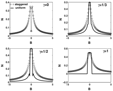
Figure 1: The negativity versus the magnetic fields for the case of two sites at a temperature of $T=0.02$.

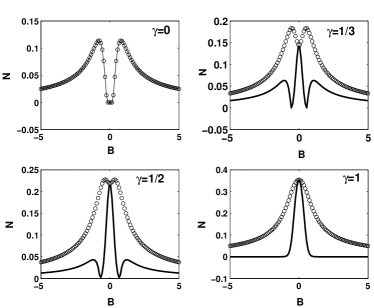
Figure 2: The negativity versus magnetic fields for the case of two sites at a temperature of $T=0.2$.

From the analytical results of the negativity, we plot the entanglement versus $B$ at a lower temperature in Fig. 1 for both the cases of the uniform and staggered fields. Throughout the paper, we use circle lines to plot the negativity versus $B$ for the case of staggered field, and solid lines for the case of uniform field. We see that the negativity is symmetric with respect to the magnetic field $B=0$, namely, $\pm B$ gives the same value of negativity. From the analytical result, changing $B$ to $-B$ results in exchanging $a_{2}$ and $a_{3}$ in Eq. (8) and exchanging $a_{1}$ and $a_{4}$ in Eq. (9). Then, from Eq. (6), we know that the negativity is invariant when changing $B$ to $-B$.

For finite anisotropic parameters, the negativity behaves differently under the two kinds of external magnetic fields. It is interesting to see that the curve for the uniform field coincides with that for the staggered field when $\gamma=0$. It can also be explained from the analytical result of the negativity. When we take $\gamma=0$ in the expressions (8) and (9), from Eq. (6), it is direct to check that the negativities are equal for the two cases of uniform and staggered magnetic fields.

Now we consider a higher temperature $T=0.2$, and the numerical results are given in Fig. 2. When $\gamma=0$, we still observe that the curve for the uniform field coincides with that for the staggered magnetic field. This is a general feature for our system, as will be shown in the following section. For $\gamma\neq 0$, the uniform field and staggered field displays different effects on entanglement, and the staggered field enhances entanglement in comparison with the case of uniform field. For $\gamma=1/3$ and $\gamma=1/2$, the negativity for the staggered field shows double peaks, while it shows triple peaks for the uniform field. This feature is dependent on the anisotropy. When $\gamma=1$, there exists only one peak as was already shown in Ref. M_Sun . How the staggered field affects entanglement in comparison with the case of uniform field relies on the anisotropic parameter. Next, we go beyond the two-qubit case, and displays some general features of entanglement in the multi-qubit anisotropic model.

III Multi-qubit model

To consider the multi-qubit model, for convenience, we restrict ourselves to the case of even number of sites. In Fig. 3, We numerically plot the negativity versus $B$ with $\gamma=0$ for even number of sites up to ten. Both the uniform and staggered field effects are considered. In this situation, the models reduce to the transverse Ising models, and again, we observe that the entanglement is symmetric with respect to $B$, and these two fields have same effects on entanglement. For finite anisotropic parameter $\gamma=0.5$ as show in Fig. 4, the behaviors of the negativity are qualitatively the same for different number of sites, namely, the uniform magnetic field leads to triple-peak structure, while the staggered field leads to the double-peak structure.

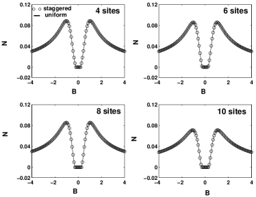
Figure 3: The negativity versus the magnetic fields for different sites. The parameters $\gamma=0$ and $T=0.2$ .

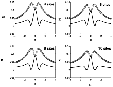
Figure 4: The negativity versus the magnetic fields for different sites. The parameters $\gamma=0.5$ and $T=0.2$ .

We first give a strict way to show that the entanglement is symmetric with respect to $B=0$. Consider the following unitary transformation

$$U_{1}=\sigma_{1x}\otimes\sigma_{2x}\otimes\sigma_{3x}\otimes...\otimes\sigma_{Nx}.$$ (10)

Then, we have

$$U_{1}H_{1}(\gamma,B)U_{1}= H_{1}(\gamma,-B),$$

$$U_{1}H_{2}(\gamma,B)U_{1}= H_{2}(\gamma,-B).$$ (11)

From the above equation, we obtain

$$U_{1}e^{-\beta H_{1}(\gamma,B)}U_{1}= e^{-\beta H_{1}(\gamma,-B)},$$

$$U_{1}e^{-\beta H_{2}(\gamma,B)}U_{1}= e^{-\beta H_{2}(\gamma,-B)}.$$ (12)

The thermal state is described by the density operator $\rho(T)=\exp(-\beta H)/Z$. The partition function is invariant under a unitary transformation of the Hamiltonian. So, the thermal state with parameter $B$ is connected with that with parameter $-B$ via the unitary transformation $U_{1}$. Another important fact is that $U_{1}$ is a local unitary operator, which will not change entanglement. Thus, the entanglement is symmetric with respect to $B=0$.

Second, we show that the uniform and staggered magnetic fields have same effects on entanglement when the anisotropic parameter $\gamma=0$. Consider the following transformation

$$U_{2}=\sigma_{1x}\otimes\sigma_{3x}\otimes\sigma_{5x}\otimes...\otimes\sigma_{N-1,x}.$$ (13)

Then, we have

$$U_{2}H_{1}(\gamma,B)U_{2}=H_{2}(-\gamma,B),$$ (14)

indicating that $U_{2}$ transform the Hamiltonian $H_{1}$ to $H_{2}$ with $\gamma$ being changed to $-\gamma$. This unitary operator is a local unitary operator, and thus will not change the entanglement. Specifically, when $\gamma=0$, we have the equality $U_{2}H_{1}(0,B)U_{2}=H_{2}(0,B)$, and thus the two magnetic fields have the same effects on entanglement.

IV Conclusion

In conclusion, we have studied the entanglement properties of the anisotropic spin-half system in a staggered external magnetic field, and compared it with the case of a uniform magnetic field. We have investigated the generic $XY$ Heisenberg model with different anisotropy $\gamma$, and have obtained the analytic results of negativity in two sites for arbitrary $\gamma$, which helped us to explain entanglement properties. We strictly show that for any temperature the entanglement is symmetric with respect to zero magnetic field, and when $\gamma=0$, the negativity for the case of staggered field is the same as that for the uniform field. If $\gamma\neq 0$ the two kinds of magnetic fields have different effects on entanglement. We have found that the staggered magnetic field leads to higher entanglement and double-peak structure. Here, we have considered the anisotropic $XY$ model, it will be interesting to consider staggered magnetic effects on entanglement in other physical magnetic models.

References

- (1) M. A. Nielsen and I. L. Chuang, Quantum Computation and Quantum Information (Cambridge University Press, Cambridge, England, 2000).
- (2) M. A. Nielsen, Ph. D thesis, University of Mexico, 1998, quant-ph/0011036.
- (3) M. C. Arnesen, S. Bose, and V. Vedral, Phys. Rev. Lett. 87, 017901 (2001).
- (4) X. Wang, Phys. Rev. A 64, 012313 (2001).
- (5) D. Gunlycke, V. M. Kendon, V. Vedral, and S. Bose, Phys. Rev. A64, 042302 (2001).
- (6) X. Wang, H. Fu, and A. I. Solomon, J. Phys. A: Math. Gen. 34, 11307(2001); X. Wang and K. Mølmer, Eur. Phys. J. D 18, 385(2002); X. Wang, Phys. Lett. A 281, 101 (2001); X. Wang and P. Zanardi, Phys. Lett. A 301, 1 (2002); X. Wang, Phys. Lett. A 329, 439 (2004).
- (7) G. L. Kamta and A. F. Starace, Phys. Rev. Lett. 88, 107901 (2002).
- (8) K. M. O’Connor and W. K. Wootters, Phys. Rev. A63, 0520302 (2001).
- (9) D. A. Meyer and N. R. Wallach, quant-ph/0108104.
- (10) Y. Sun, Y. G. Chen, and H. Chen, Phys. Rev. A 68, 044301 (2003).
- (11) C. Anteneodo and A. M. C. Souza, J. Opt. B: Quantum Semi-class. Opt. 5, 73 (2003).
- (12) P. Štelmachovič and V. Bužek, Phys. Rev. A 70, 032313 (2004).
- (13) L. F. Santos, Phys. Rev. A67, 062306 (2003).
- (14) Y. Yeo, Phys. Rev. A66, 062312 (2002).
- (15) D. V. Khveshchenko, Phys. Rev. B68, 193307 (2003).
- (16) L. Zhou, H. S. Song, Y. Q. Guo, and C. Li, Phys. Rev. A68, 024301 (2003).
- (17) J. Schliemann, Phys. Rev. A68, 012309 (2003).
- (18) L. Zhou, X. X. Yi, H. S. Song, and Y. Q. Guo, quant-ph/0310169.
- (19) Y. Q. Li and G. Q. Zhu, submitted.
- (20) G. K. Brennen, S. S. Bullock, quant-ph/0406064.
- (21) G. Tóth and J. I. Cirac, quant-ph/0406061.
- (22) A. Osterloh, L. Amico, G. Falci, and R. Fazio, Nature (London) 416, 608 (2002).
- (23) T. J. Osborne and M. A. Nielsen, Phys. Rev. A66, 032110 (2002).
- (24) S. J. Gu, H. Q. Lin, and Y. Q. Li, Phys. Rev. A68, 042330 (2003); S. J. Gu, G. S. Tian, and H. Q. Lin, quant-ph/0408101; S. J. Gu, S. S. Deng, Y. Q. Li, and H. Q. Lin, Phys. Rev. Lett. 93, 086402 (2004).
- (25) U. Glaser, H. Büttner, H. Fehske, Phys. Rev. A68, 032318 (2003).
- (26) O. F. Syljuåsen, Phys. Rev. A68, 060301 (2003).
- (27) F. Verstraete, M. Popp, and J. I. Cirac, Phys. Rev. Lett. 92, 027901 (2004).
- (28) F. Verstraete, M. A. Martin-Delgado, J. I. Cirac, Phys. Rev. Lett. 92, 087201 (2004).
- (29) J. Vidal, G. Palacios, and R. Mosseri, Phys. Rev. A 69, 022107 (2004).
- (30) N. Lambert, C. Emary, and T. Brandes, Phys. Rev. Lett. 92, 073602 (2004).
- (31) Y. Chen, P. Zanardi, Z. D. Wang, and F. C. Zhang, quant-ph/0407228.
- (32) K. Audenaert, J. Eisert, M. B. Plenio, and R. F. Werner, Phys. Rev. A66, 042327 (2002); M.B. Plenio, J. Hartley, and J. Eisert, New J. Phys. 6, 36 (2004).
- (33) L. A. Wu, M. S. Sarandy, and D. A. Lidar, quant-ph/0407056.
- (34) G. Vidal, J. I. Latorre, E. Rico, and A. Kitaev Phys. Rev. Lett. 90, 227902 (2003).
- (35) S. Ghose, T. F. Rosenbaum, G. Aeppli, and S. N. Coppersmith, Nature (London) 425, 48 (2003).
- (36) S. Bose, Phys. Rev. Lett. 91, 207901 (2003); V. Subrahmanyam, Phys. Rev. A69, 034304 (2004); M. Christandl, N. Datta, A. Ekert, and A. J. Landahl, Phys. Rev. Lett. 92, 187902 (2004); Y. Li, T. Shi, Z. Song, and C. P. Sun, quant-ph/0406159; M. B. Plenio and F. L Semião, quant-ph/0407034.
- (37) A. Peres, Phys. Rev. Lett. 77, 1413 (1996); M. Horodecki, P. Horodecki, and R. Horodecki, Phys. Lett. A 223, 1 (1996).
- (38) G. Vidal and R. F. Werner, Phys. Rev. A65, 032314 (2002).