A Single Photon Source With Linear Optics and Squeezed States

Abstract

Quantum information processing using photons has recently been stimulated by the suggestion to use linear optics, single photon sources and detectors. The recent work by Knill has also shown that errors in photon detectors leads to a high error rate threshold (around $29\%$). An important missing element are good single photon sources. In this paper we show how to make a single photon source using squeezed states, linear optics and conditional measurement. We use degenerate squeezed vacuum states, in contrast to the normal non-degenerate squeezed vacuum states used for single photon production. We show that we can get a photon with certainty when detectors click appropriately, the last event happening up to around $25\%$ of the time. We also show the robustness of this method with respect to a variety of potential imperfections.

Quantum mechanics provides a new way to manipulate and encode information that has no classical counterpart. This has lead to new algorithms, cryptographic protocols, higher precision measuring techniques and more. Many proposals have been put forward to build devices that will be able to harness the quantum world and turn the theoretical advantage of using quantum mechanics into a practical one areview . Quantum optics has demonstrated a high control of the quantum world because photons interact weakly with each other and thus have long decoherence times. Demonstration of quantum cryptography abound and have even lead to prototypes which are presently reaching the market. However these devices have severe limitation in the distance over which they can be used. To go beyond these first prototypes by extending the maximum distance they can be deployed or to increase their reliability, better control of the quantum systems must be achieved in order to be able to implement quantum repeaters and error correction schemes. Such schemes require quantum gates and interaction between photons.

Photons interact in media through what is called the Kerr effect, but typically this interaction is much too weak for quantum information purposes. One of the first experimental demonstrations of quantum gates used cavity QED mediated interaction of photons Turchette . It was a nice proof of principle but it was however quickly realized that it would be difficult to scale beyond a few gates.

Recently it has been proposed to use single photon sources, detectors and linear optics KLM for quantum information processing. This suggestion uses projection of the quantum states and feedback to simulate efficiently the quantum circuit model. Progress in LOQC has been made in two fronts. Proof-of-principle experiments, demonstrating that the fundamental elements have been realized Obrien ; Pittman ; Sanaka ; Fattal . These show that today we have sufficient control to manipulate small quantum systems. The second avenue of progress has been to assess the constraint in precision of the elements required for LOQC. Linear optical elements, beam splitters and phase shifters, can be made with high accuracy and are very reliable. These could without too much difficulty reach the threshold accuracy for generic error threshold in order to compute reliably using quantum error correction. It was shown in knill:qc2003 that, if only errors in detectors were present, an accuracy threshold around $70\%$ was sufficient. A similar calculation with a different set of assumptions showed an error threshold around $2\%$ Silva . Finally, although a lot of effort has been put into making single photon sources, none are yet of a quality sufficient for making the linear optics proposal scalable. In this letter we propose a new way to devise such a source based on the idea of linear optics.

The purpose of this paper is to propose a single photon source that can be improved dramatically using the ideas of LOQC and error correction, i.e. we are asking if it is possible to use a set of imperfect sources, make them interfere through beam splitters and phase shifters, detect some of the output, and improve the amplitude of observing a single photon. It turns out that it seems impossible if the input is in a mixture of the state $|0\rangle$ and $|1\rangle$ Imamoglu ; Berry04:1 ; Berry04:2 . On the other hand, if the source is coherent it is however possible.

If three identical copies of the state $\alpha|0\rangle+\beta|1\rangle$ are put onto the two beam splitter system Berry04:2 shown in figure (1), we are able to condition off of certain detections to have, with certainty, the state $|1\rangle$ in the output mode. This input state can be written as $\Bigl{(}(\alpha+\beta\hat{a}^{\dagger})|0\rangle\Bigr{)}^{\otimes 3}$. We use the beam splitter transformation KLM : $\hat{a}_{l}^{\dagger}\rightarrow\sum_{k}\Lambda_{kl}\hat{a}_{k}^{\dagger}$, where

$$\bm{\Lambda}=\left[\begin{array}[]{*{20}c}\cos{\theta}&-e^{i\phi}\sin{\theta}\\ e^{-i\phi}\sin\theta&\cos\theta\\ \end{array}\right]$$ (1)

If we condition off detecting “2” photons in mode 2 and “0” photons in mode 3 the state in mode 1 is (un-normalised)

$$\beta^{2}\Lambda_{22}^{\prime}[\alpha\bigl{(}\Lambda_{23}\Lambda_{21}^{\prime}+\Lambda_{22}(\Lambda_{21}^{\prime}+\Lambda_{23}\Lambda_{22}^{\prime})\bigr{)}|0\rangle$$

$$+\beta\Lambda_{22}\Lambda_{23}\bigl{(}2\Lambda_{12}^{\prime}\Lambda_{21}^{\prime}+\Lambda_{11}^{\prime}\Lambda_{22}^{\prime}\bigr{)}|1\rangle]$$ (2)

By choosing the angles of both beam splitters to be a function of the beam splitter phases $\phi$ and $\nu$ (see figure (1)), we can set the coefficient in front of $|0\rangle$ in (A Single Photon Source With Linear Optics and Squeezed States) to 0 for: $\theta=\arctan\bigl{(}\frac{\sin(\nu+\phi)}{\sin(\nu)}\bigr{)}$, $\mu=-\arctan\bigl{(}\frac{\sin(\nu+\phi)\sin(\nu)}{\sin(\phi)\sqrt{\sin^{2}(\nu)+\sin^{2}(\phi+\nu)}}\bigr{)}$. The maximum probability of a “2” “0” detection is $\frac{16|\beta|^{3}}{81}$ (but note that when we have these detections we insure having a single photon).

The difficulty is reduced to make a state of the form $\alpha|0\rangle+\beta|1\rangle$. Instead of such a state let’s concentrate on a squeezed coherent state. This has the form $|\xi,\alpha\rangle=\frac{\exp[-\frac{1}{2}(|\alpha|^{2}-\alpha^{2}\tanh r)]}{\sqrt{\cosh r}}\sum_{n=0}^{\infty}\frac{1}{\sqrt{n!}}\Biggl{(}\sqrt{\frac{\sinh r}{2\cosh r}}\Biggr{)}^{n}\times H_{n}\Bigl{(}\frac{\alpha}{\sqrt{2\cosh r\sinh r}}\Bigr{)}|n\rangle$ where $\xi=re^{i\varphi}$. As shown in Matsuoka , we can set the 2 photon term to zero by setting the 2nd Hermite polynomial $H_{2}(x)$ to 0. Using this method we could generate states with a probability of production equal to $1.2\%$ and a single photon content as high as $96.5\%$ at the highest yet attainable squeezing ($r=0.36$ Wenger ). As we increase the squeezing (with the displacement length changing according to $\alpha=\sqrt{\frac{\sinh(2r)}{2}}$ so that $H_{2}(x)=0$), the probability of production increases until $r=0.81$, after which it begins to drop towards 0. Also, as we increase the squeezing, the single photon content percentage asymptotes to a value of $82\%$. The problem with this scheme is that there is no way to rid ourselves of higher order photon terms.

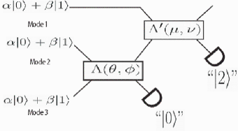
Figure 1: Show the system to get a single photon from three identical known copies of the state $\alpha|0\rangle+\beta|1\rangle$.

The above analysis motivates us to look at squeezed states as inputs into linear optical systems to try and better current single photon sources. Squeezed states are considered to be Gaussian states, the simplest type of Gaussian state is the coherent state, having many similarities to a classical description of a field. A coherent state is defined by Walls $|\alpha\rangle=\exp{(\alpha\hat{a}^{\dagger}-\alpha^{*}\hat{a})}|0\rangle$, where $a^{\dagger}|n\rangle=\sqrt{n+1}|n+1\rangle$. The light from a stabilized laser is a typical example of a coherent state Ralph . The Wigner function of a coherent state is given by Walls $W(x_{1}^{\prime},x_{2}^{\prime})=\frac{2}{\pi}\exp\Bigl{(}-\frac{1}{2}(x_{1}^{\prime 2}+x_{2}^{\prime 2})\Bigr{)}$, where $x_{i}^{\prime}=x_{i}-X_{i}$ and $X_{1}$ and $X_{2}$ play the role of non-commuting electric field quadrature observables: $\hat{a}=\frac{1}{2}\bigl{(}X_{1}+iX_{2}\bigr{)}$. As can be seen a coherent state is a Gaussian in phase space centred at $(X_{1},X_{2})$ with an equal distribution in all directions, that is a coherent state has minimum uncertainty in both the position and the momentum quadrature.

Squeezed states also have a minimum Heisenberg uncertainty but with the uncertainty in one direction reduced at the expense of the uncertainty in the other direction. A squeezed vacuum is defined by

$$|\xi\rangle =\exp\Bigl{(}\frac{\xi}{2}(\hat{a}^{\dagger})^{2}-\frac{\xi^{*}}{2}(\hat{a})^{2}\Bigr{)}|0\rangle$$ (3)

where $\xi=r\exp{(i\varphi)}$ governs the amount and orientation of squeezing. The Wigner function for a squeezed state, squeezed along one of the quadrature axes, is given by Walls $W(x_{1}^{\prime},x_{2}^{\prime})=\frac{2}{\pi}\exp\Bigl{(}-\frac{1}{2}(x_{1}^{\prime 2}e^{-2r}+x_{2}^{\prime 2}e^{2r})\Bigr{)}$. This is also a Gaussian state centred at $(X_{1},X_{2})$ but instead of a circle in phase space, as with a coherent state, it is an ellipse, with minor and major axes given by $\exp(r)$ and $\exp(-r)$, respectively.

Squeezed states are produced when coherent light interacts with a nonlinear medium, such as in degenerate parametric down conversion Wu86 . Squeezing can be achieved with either cw Polzik or pulsed light Slusher , and this normally dictates what type of measurement is allowable. It is only the latter type of squeezing, that is pulsed squeezing, that allows the use of photon counting detectors. It is for this reason that we consider pulsed squeezing in this letter. To date the best cw squeezing achieved is 7.2dB Schneider . This corresponds to $r=0.83$. In contrast the best pulsed squeezing recorded is 3.1dB Wenger , corresponding to $r=0.36$. This is approximately an ellipse in phase space with a minor axis $\frac{1}{2}$ the size of the major axis.

The squeezed vacuum state given in Eqn.(3) is equal to Barnett ; Vogel

$$|\zeta\rangle=\frac{1}{\sqrt{\cosh{r}}}\exp[-\frac{1}{2}\exp(i\varphi)\tanh(r)(\hat{a}^{\dagger})^{2}]|0\rangle$$ (4)

If we put two of these states ($|\xi_{1}\rangle\otimes|\xi_{2}\rangle$) onto a beam splitter BS2, as shown in figure (2), the term in the exponent becomes

$$\Bigl{(}\lambda_{1}\Lambda_{11}^{2}+\lambda_{2}\Lambda_{12}^{2}\Bigr{)}(\hat{a}_{1}^{\dagger})^{2} + 2\Bigl{(}\lambda_{1}\Lambda_{11}\Lambda_{21}+\lambda_{2}\Lambda_{12}\Lambda_{22}\Bigr{)}\hat{a}_{1}^{\dagger}\hat{a}_{2}^{\dagger}$$ (5)

$$+ \Bigl{(}\lambda_{1}\Lambda_{21}^{2}+\lambda_{2}\Lambda_{22}^{2}\Bigr{)}(\hat{a}_{2}^{\dagger})^{2}$$

where $\xi_{j}=r_{j}\exp(i\varphi_{j})$ and $\lambda_{j}=-\frac{1}{2}\exp(i\varphi_{j})\tanh(r_{j})$, $j\in\{1,2\}$.

If we detect off measuring a “1” in mode 2 this becomes:

$$\frac{2}{\sqrt{\cosh(r_{1})\cosh(r_{2})}}\Bigl{(}\lambda_{1}\Lambda_{11}\Lambda_{21}+\lambda_{2}\Lambda_{12}\Lambda_{22}\Bigr{)}\hat{a}_{1}^{\dagger}$$

$$\times\exp[\Bigl{(}\lambda_{1}\Lambda_{11}^{2}+\lambda_{2}\Lambda_{12}^{2}\Bigr{)}(\hat{a}_{1}^{\dagger})^{2}]|00\rangle$$ (6)

In order to have a perfect single photon source we need $\lambda_{1}\Lambda_{11}^{2}+\lambda_{2}\Lambda_{12}^{2}=0$. If we assume identical squeezed vacuum states such that $\lambda_{1}=\lambda_{2}$ and a symmetric beam splitter ($\theta=\frac{\pi}{4},\phi=\frac{\pi}{2}$) this gives a single photon. Putting these numbers into Eqn.(5) gives the equivalent of a two mode squeezed vacuum Barnett . Producing a two mode squeezed vacuum this way is advantageous for a few reasons, one being that the intensity of the pump beams need not be as high as that for non-degenerate down conversion.

Before any detections, the state after BS2 in figure (2) is

$$\frac{1}{\cosh(r)}\exp[i\exp(i\varphi)\tanh(r)\hat{a}_{1}^{\dagger}\hat{a}_{2}^{\dagger}]|00\rangle$$ (7)

From (7) we can see that the probability of detecting $n$ photons in mode 2 is given by

$$\text{Prob.}=\frac{\tanh^{2n}(r)}{\cosh^{2}(r)}$$ (8)

The maximum probability to observe a single photon is $25\%$ at a squeezing of $r_{\text{max}}=0.88137$. With todays technology a squeezing of $r=0.36$ is possible Wenger , corresponding to a single photon probability of $10.5\%$.

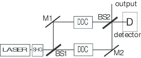
Figure 2: Setup to allow two squeezed vacuum states onto a beam splitter. SGH = second harmonic generation, M = mirror, BS = beam splitter and DDC = degenerate down conversion. BS1 is a symmetric 50:50 beam splitter, as is BS2 ($\theta=\frac{\pi}{4},\phi=\frac{\pi}{2}$). The dotted box indicates an inefficient detector.

One problem that our scheme will face is mode mismatch on BS2. However it is possible to take this into account, as shown in Banaszek .

Next we consider how robust our proposed single photon source is against an inefficient detector. We model our inefficient detector with a beam splitter of reflectivity $\eta$ in front of an ideal detector Yurke ; Kiss . When $\eta=1$ we have a perfect detector and when $\eta=0$ the detector no longer detects

We calculate the probability of measuring a single photon at the ideal detector by taking into account that there may be more than 1 photon present, so many terms will give rise to a single photon event on our ideal detector, each with some probability. This gives the probability of measuring 1 click on our detector and having the state $|n\rangle$ output as $\text{P}_{n}=n\eta\bigl{(}1-\eta\bigr{)}^{n-1}\frac{\tanh^{2n}(r)}{\cosh^{2}(r)}$. The total probability $\text{P}^{d}_{1}$ of our inefficient detector to click for a single photon is given by

$$\text{P}^{d}_{1}=\sum_{n=1}^{\infty}\text{P}_{n}=\frac{4\eta\sinh^{2}(r)}{\bigl{(}2-\eta+\eta\cosh(2r)\bigr{)}^{2}}$$ (9)

This is shown as the red line in figure (3). In such a case the probability of having a single photon in the output becomes

$$\text{P}^{p}_{1}=\frac{(2-\eta+\eta\cosh 2r)^{2}}{4\cosh^{4}r}$$ (10)

shown as the blue line in figure (3).

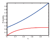
Figure 3: Shows the probability of measuring a single photon with an inefficient detector (red) and the probability of observing a single photon in the output given we measure a single photon (blue). Here $r=r_{\text{max}}$.

We now consider dark counts for the inefficient detector in figure (2). From Banaszek it can be shown that the probability for 1 click when we take dark counts into account is given by $\text{P}_{1}^{\text{dark}}=p_{d}+(1-p_{d})\langle\hat{P}_{1}\rangle=\langle p_{d}\cdot\mathbb{I}+(1-p_{d})\hat{P}_{1}\rangle$, where $\hat{P}_{1}=\sum_{n=1}^{\infty}P_{n}|n\rangle\!\langle n|$ and $p_{d}$ is the probability of a dark count. Using the fact that $\mathbb{I}=\sum_{n=0}^{\infty}|n\rangle\!\langle n|$ we find the total probability to detect a photon to be

$$p_{d}+\frac{4(p_{d}-1)}{(2-\eta+\eta\cosh 2r)^{2}}-\frac{2(p_{d}-1)}{2-\eta+\eta\cosh 2r}$$ (11)

and the probability to have a single photon output conditioned on detecting a single photon is

$$\frac{(p_{d}(\eta-1)-\eta)(2-\eta+\eta\cosh 2r)^{2}\text{sech}^{2}r\tanh^{2}r}{p_{d}(4+(\eta-2)\eta)-2\eta+\eta\cosh 2r(2-2p_{d}(\eta-1)+p_{d}\eta\cosh 2r)}$$ (12)

We plot the total probability (Eqn.(11)) in figure (4a) and the conditioned single photon output probability (Eqn.(12)) in figure (4b).

(a)                               (b)

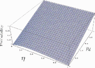
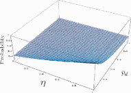
Figure 4: (a): Shows the probability of observing a detector click when we take dark counts into account for our inefficient detector. (b): Conditional probability of a single photon in the output. Here $r=r_{\text{max}}$.

Next we consider a beam splitter that has some uncertainty in the reflectivity. Instead of the usual beam splitter matrix (1) we consider the case when the angles $\theta$ and $\phi$ have perturbations given by: $\theta\mapsto\theta+\delta_{1}$, $\phi\mapsto\phi+\delta_{2}$. When we condition off observing a single photon in the detector the state in the output mode becomes: $|\psi\rangle_{\text{badBS}}=\mathcal{A}_{1}\hat{a}_{1}^{\dagger}\exp[\mathcal{B}_{1}(\hat{a}_{1}^{\dagger})^{2}]|0\rangle$ where $\mathcal{A}_{1}=ie^{(i\varphi)}\frac{\tanh(r)}{2\cosh(r)}\Bigl{(}\cos^{2}\delta_{1}-\sin^{2}\delta_{1}\Bigr{)}\Bigl{(}e^{(-i\delta_{2})}+e^{(i\delta_{2})}\Bigr{)}$ and $\mathcal{B}_{1}=-\frac{1}{4}e^{(i\varphi)}\tanh(r)\Bigl{(}\bigl{(}\cos\delta_{1}-\sin\delta_{1}\bigr{)}^{2}-e^{(2i\delta_{2})}\bigl{(}\cos\delta_{1}+\sin\delta_{1}\bigr{)}^{2}\Bigr{)}$. We see that the probability of having a single photon on the condition of a click in the detector is

$$\text{P}^{\text{BS}}_{1}=\frac{1}{\sum_{n=0}^{\infty}\frac{(2n+1)!}{(n!)^{2}}||(\mathcal{B}_{1})^{n}||^{2}}$$ (13)

We see that the probability of observing $n$ photons in mode 1 is given by

$$\frac{(2n+1)!}{(n!)^{2}}||\mathcal{A}_{1}(\mathcal{B}_{1})^{n}||^{2}$$ (14)

The probability of a single photon state output in mode 1 as a function of $\delta_{1}$ and $\delta_{2}$ is graphed in the figure (5). In figure (5a) we show the probability of observing 1 photon in mode 1 (Eqn.(14)) and in figure (5b) we show the probability of having a single photon conditioned on a single photon detection (Eqn.(13)).

(a)                               (b)

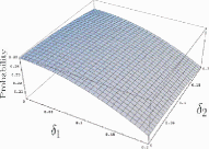
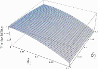
Figure 5: (a): Shows a probability of observing $|1\rangle$ in mode 1 as a function of the beam splitter perturbation $\delta_{1}$ and $\delta_{2}$ (b): Shows a probability of observing $|3\rangle$ in mode 1. Here $r=r_{\text{max}}$.

In conclusion, we have proposed a single photon source using pulsed degenerate squeezed vacuum states, linear optics and conditional measurements. We have shown that we can in theory get a certified single photon at every four attempts, with today’s achieved value of pulse squeezing this reduces to ten attempts. We have also shown that this process is robust under various imperfections.

We thank M. Knill, A. Imamoglu, B.C. Sanders, D. Berry, G.J. Milburn and K. Banaszek for useful interaction. CRM and RL are supported in part by CIAR, NSERC, RL is also supported in part by ORDCF and the Canada Research Chair program and ME would like to thank the Swedish Research Council for financial support and also Björn Hessmo for useful discussions. RL and ME thank the Newton Institute.

References

- (1) R. Laflamme et. al., The Physics of Quantum Computing, special volume, ed H. Everitt, Quantum Information Processing, to appear, e-print quant-ph/0207172.
- (2) Q.A. Turchette, C.J. Hood, W. Lange, H. Mabuchi and H.J. Kimble, Phys. Rev. Lett. 75, 4710 (1995).
- (3) E. Knill, R. Laflamme and G.J. Milburn, Nature 409, 46 (2001).
- (4) J. L. O’Brien, G.J. Pryde, A.G. White, and T.C. Ralph, Nature 426, 264 (2003).
- (5) T.B. Pittman, M.J. Fitch, B.C. Jacobs, and J.D. Franson, Phys. Rev. A. 68, 032316 (2003).
- (6) K. Sanaka, T. Jennewein, J.-W. Pan, K. Resch, and A. Zeilinger, Phys, Rev. Lett. 92, 017902 (2004).
- (7) D. Fattal, E. Diamanti, K. Inoue, and Y. Yamamoto, Phys. Rev. Lett. 92, 037904 (2004).
- (8) D. Aharonov and M. Ben-Or, Proc. 29th Ann. ACM Symp. on Theory of Computation (ACM, New York, 1998), pp. 176-188, quant-ph/9611025; A. Y. Kitaev, Proc. 3rd Int. Conf. of Quantum Communication and Measurement (Plenum Press, New York, 1997), pp. 181-188; E. Knill, R. Laflamme, and W.H. Zurek, Science 279, 342 (1998); J. Preskill, Proc. Soc. Roy. Lond. A 454, 385 (1998).
- (9) E. Knill, e-print quant-ph/0312190.
- (10) M. Silva, M.Sc. Thesis, e-print quant-ph/0405112.
- (11) A. Imamoglu and E. Knill, private correspondence.
- (12) D.W. Berry, S. Scheel, B.C. Sanders and P.L. Knight, Phys. Rev. A 69, 031806(R) (2004).
- (13) D.W. Berry, S. Scheel, C.R. Myers, B.C. Sanders, P.L. Knight and R. Laflamme, New J. Phys. 6, 93 (2004).
- (14) Matsuoka and Hirano, Phys. Rev. A 67, 042307 (2003)
- (15) D.F. Walls and G.J. Milburn, Quantum Optics, Springer-Verlag, Berlin, (1994).
- (16) T.C. Ralph, A. Gilchrist, G.J Milburn, W.J. Munro and S. Glancy, Phys. Rev. A 68, 024319 (2003).
- (17) L.-A. Wu, H.J. Kimble, J.L. Hall and H. Wu, Phys. Rev. Lett. 57, 2520 (1986).
- (18) E.S. Polzik, J. Carri and H.J. Kimble, Appl. Pys. B: Photophys. Laser Chem. 55, 279 (1992).
- (19) R.E. Slusher, P. Grangier, A. LaPorta, B. Yurke and M.J. Potasek, Phys. Rev. Lett.59, 2566 (1987).
- (20) K. Schneider, M. Lang, J. Mlynek and S. Schiller, Optics Express 2, 59 (1997).
- (21) J. Wenger, R. Tualle-Brouri and P. Grangier, Phys. Rev. Lett. 92, 153601 (2004).
- (22) S. M. Barnett and P.M.Radmore, Methods in Theoretical Quantum Optics, Oxford University Press, Oxford, U.K. (1997).
- (23) W. Vogel, D.-G. Welsch and S. Wallentowitz, Quantum Optics An Introduction 2nd revised and enlarged edition (Wiley-VCH, Berlin, 2001).
- (24) B. Sandes, P. Knight etc Journal 273, 1073 (1996).
- (25) K. Banaszek, A. Dragan, K. Wodkiewicz and C. Radzewicz, Phys. Rev. A 66, 043803 (2002).
- (26) B. Yurke, Phys. Rev. A 32, 311 (1985).
- (27) T. Kiss, U. Herzog and U. Leonhardt, Phys. Rev. A 52, 2433 (1995).