Algorithm-Based Analysis of Collective Decoherence in Quantum Computation

Abstract

The information in quantum computers is often stored in identical two-level systems (spins or pseudo-spins) that are separated by a distance shorter than the characteristic wavelength of a reservoir which is responsible for decoherence. In such a case, the collective spin-reservoir interaction, rather than an individual spin-reservoir interaction, may determine the decoherence characteristics. We use computational basis states, symmetrized spin states and spin coherent states to study collective decoherence in the implementation of various quantum algorithms. A simple method of implementing quantum algorithms using stable subradiant states and avoiding unstable Dicke’s superradiant states and Schrödinger’s cat states is proposed.

I Introduction

In future quantum information processing systems, quantum bits (qubits) of information are likely to be stored in identical two-level systems (spins or equivalent spins) that are spatially separated to simultaneously allow independent control of single qubits and mutual interaction between qubits. If a system of $n$ spins interacts with a reservoir whose characteristic wavelength is longer than the inter-spin distance, the system interacts collectively with the bath. For instance, electron-spin-based quantum computers Loss and DiVincenzo (1998) have an inter-spin distance on the order of 10 to 100 nm, which can be far shorter than the wavelength of a coupled low temperature phonon reservoir. Another example is a nuclear-spin-based quantum computer using doped impurities Kane (1998) or a crystal lattice Yamaguchi and Yamamoto (1998); Ladd et al. (2002) in which a remote paramagnetic impurity interacts with a nuclear spin system by a long-range dipolar coupling Slichter (1990). If the distance between qubits is much smaller than their separation from the impurity, the interaction can also be treated as collective.

In theory, if a system-bath interaction exhibits a high degree of symmetry, computation can be performed in a decoherence-free subspace (DFS) that leaves the logical qubits immune to the influence of the bath Kitaev ; Palma et al. (1996); Duan and Guo (1998); Zanardi and Rasetti (1997); Zanardi (1998); Lidar et al. (1998); Knill et al. (2000); Lidar and Whaley . However, if one restricts logical states to this subspace, it is difficult to design simple gates to implement quantum algorithms. Consider, by comparison, a standard model of quantum computation, which labels logical states (computational basis states) by the tensor-products of the two-level qubit states, and implements the unitary evolution for a given algorithm by a sequence of controlled-NOT (CNOT) gates and single-qubit rotations. These fundamental gates are physically convenient, as they can be created simply through pairwise interactions between qubits and local control pulses (i.e., by exploiting the innate tensor product structure of the Hilbert space). By contrast, if logical states are defined within a DFS, the control sequences are complicated by the requirement that the state does not wander out of the DFS during evolution. Thus, in the interest of simple gate construction, we examine decoherence in the context of the standard computational basis and the full Hilbert space.

Consider the unitary evolution of a quantum computer during the course of a given algorithm. Ideally, the state is described by a trajectory in the $2^{n}$-dimensional complex Hilbert space. If a collective system-environment interaction is present, the instantaneous decoherence rate can be parameterized by the “proximity” of the ideal trajectory to the decoherence-free subspace, allowing us to infer how the decoherence rate evolves over the course of the algorithm. Generally, the end result of a quantum algorithm is encoded in the measurement of the final state; there is thus some freedom to choose an initial state and/or trajectory that minimizes the average proximity to the DFS. In this fashion, one can attempt to minimize the impact of decoherence due to the collective system-reservoir interaction while maintaining the simplicity of the tensor-product structure of the full Hilbert space. As a compromise between a naive application of the standard model and logical encoding in a DFS, this approach might be useful to implement algorithms on a prototype quantum computer, where the number of qubits is too modest to implement quantum error correction.

In this paper, we introduce physical models for collective spin-reservoir interactions, and examine relevant parameterizations of the decoherence rate during the time evolution of specific useful quantum algorithms. It is shown that judicious choice of the initial state or gate sequence can often reduce the decoherence rate parameter significantly.

A collective spin-reservoir interaction that is responsible for a longitudinal relaxation process ($T_{1}$ process) can be modeled by

$$\hat{\mathcal{H}}_{I}=\sum_{i}\hbar k_{i}\left(\hat{a}_{i}^{\dagger}\hat{J}^{-}+\hat{a}_{i}\hat{J}^{+}\right).$$ (1)

Here, $\hat{a}_{i}$ ($\hat{a}_{i}^{\dagger}$) is an annihilation (creation) operator of the bosonic reservoir and $\hat{J}^{+}$ ($\hat{J}^{-}$) is a collective raising (lowering) operator of the spin system:

$$\hat{J}^{\pm}=\sum_{\ell=1}^{n}\hat{J}^{\pm}_{\ell}=\frac{1}{2}\sum_{\ell=1}^{n}\sigma^{\pm}_{\ell},$$ (2)

where $\hat{\sigma}^{\pm}_{\ell}=\hat{\sigma}_{\ell}^{x}\pm i\hat{\sigma}_{\ell}^{y}$ are Pauli operators for spin $\ell$.

In this model, the longitudinal relaxation time $T_{1}$ can be much shorter than that for a single isolated spin; this phenomenon is known as superradiant decay in atomic physics Dicke (1954). In contrast, the so-called subradiant states have negligible $1/T_{1}$. To characterize this longitudinal relaxation rate, it will be useful to define simultaneous eigenstates of the squared total angular momentum $\hat{J}^{2}$ and the z-component $\hat{J}^{z}$ of the total angular momentum $\hat{J}$, notated symmetrized spin states, and discussed further in Sec. II.2. By projecting the ideal trajectory onto the symmetrized states, we can calculate a time-dependent parameter to estimate the $T_{1}$ relaxation rate.

The collective spin-reservoir interaction that we adopt to model transverse relaxation ($T_{2}$) processes is

$$\mathcal{H}_{I}=\sum_{i}\hbar g_{i}\hat{a}^{+}_{i}\hat{a}_{i}\hat{J}^{z}.$$ (3)

Here $\widehat{J}^{z}$ is the z-component of the total angular momentum $\widehat{J}$,

$$\widehat{J}^{z}=\sum^{N}_{j=1}\widehat{J}_{j}^{z}=\frac{1}{2}\sum^{n}_{j=1}\widehat{\sigma}_{j}^{z}\ \ .$$ (4)

In order to gain a physical picture for the collective $T_{1}$ and $T_{2}$ decoherence behaviors in an $N$ spin system, it is convenient to use a spin coherent state which is a linear superposition of symmetrized spin states with the same total angular momentum $j$ and the third quantum number $\alpha$ Bonifacio et al. (1969); Arecchi et al. (1972). The $Q(\alpha)$ representation of the spin state in terms of spin coherent states can easily identify a macroscopically separated linear superposition state which is subject to strong collective decoherence.

We will examine for modest $n$ the collective decoherence properties of two representative quantum algorithms: the Deutsch-Josza algorithm Deutsch and Jozsa (1992) and quantum search Grover (1997). We find a few cases in which the system state must pass through vulnerable states, such as Dicke’s superradiant states and macroscopically separated linear superposition states, and so is vulnerable to rapid longitudinal relaxation and transverse relaxation due to large instantaneous coupling to the external reservoir. We propose that simple modifications to the algorithms can avoid this problem.

II Computational Basis States, Symmetrized Spin States and Spin Coherent States

In this section, we introduce three sets of basis states. The first set is a standard computational basis formed by the tensor product of $n$ two-level systems, and is most natural in discussing gate-by-gate implementations of various algorithms. The second basis set consists of symmetrized states that are convenient to calculate collective longitudinal and transverse relaxation rates. The third is a set of spin coherent states that is suitable to discuss $Q(\theta,\varphi)$ representation.

II.1 Computational basis states

In accordance with the standard model describing the state of $n$ spin-1/2 qubits, computational basis states are defined as simultaneous eigenstates of $\left\{\hat{J}_{1}^{2},\hat{J}_{2}^{2},\ldots,\hat{J}_{n}^{2};\hat{J}_{1}^{z},\hat{J}_{2}^{z},\ldots,\hat{J}_{n}^{z}\right\}$:

$$\widehat{J}_{i}^{2}|j_{1},j_{2},\dotsm,j_{n};m_{1},m_{2},\dotsm,m_{n}\rangle\hskip 70.0pt$$

$$\hskip 20.0pt=j_{i}(j_{i}+1)|j_{1},j_{2},\dotsm,j_{n};m_{1},m_{2},\dotsm,m_{n}\rangle$$ (5a)

$$\widehat{J}_{i}^{z}|j_{1},j_{2},\dotsm,j_{n};m_{1},m_{2},\dotsm,m_{n}\rangle\hskip 70.0pt$$

$$\hskip 20.0pt=m_{i}|j_{1},j_{2},\dotsm,j_{n};m_{1},m_{2},\dotsm,m_{n}\rangle\ ,$$ (5b)

where $j_{i}=1/2$ and $m_{i}=\pm 1/2$. As all the $j_{i}$ values are fixed for a collection of two-level spins, we omit them in denoting a computational basis state. Thus, the Hilbert space is spanned by the $2^{n}$ basis states $\left|m_{1},m_{2},\ldots,m_{n}\right>$.

II.2 Symmetrized spin states

II.2.1 Definition

Symmetrized spin states are defined as simultaneous eigenstates of $\left\{\hat{J}_{1}^{2},\hat{J}_{2}^{2},\ldots,\hat{J}_{n}^{2};\hat{J}^{2},\hat{J}^{z}\right\}$:

$$\hat{J}_{i}^{2}\left|j_{1},j_{2},\ldots,j_{n};j,m\right> =j_{i}(j_{i}+1)\left|j_{1},j_{2},\ldots,j_{n};j,m\right>$$ (6a)

$$\hat{J}^{2}\left|j_{1},j_{2},\ldots,j_{n};j,m\right> =j(j+1)\left|j_{1},j_{2},\ldots,j_{n};j,m\right>$$ (6b)

$$\hat{J}^{z}\left|j_{1},j_{2},\ldots,j_{n};j,m\right> =m\left|j_{1},j_{2},\ldots,j_{n};j,m\right>$$ (6c)

We again omit the $j_{i}$ labels from the symmetrized states. Note that $j\in\{0,1,2,\ldots,n/2\}$ for $n$ even and $j\in\{1/2,3/2,\ldots,n/2\}$ for $n$ odd, and $m\in\left\{-j,-j+1,\ldots,j\right\}$. Generally, each symmetrized state $\left|j,m,\alpha\right>$ is $d$-fold degenerate; $\alpha\in\left\{1,2,\ldots,d\right\}$ encapsulates all other quantum numbers required to distinguish each basis state. Symmetrized spin states can be linearly expanded in terms of computational basis states via Clebsch-Gordan coefficients, whose properties are summarized in Appendix A.

II.2.2 Collective longitudinal relaxation rate

To gauge the impact of the longitudinal relaxation process described by Eq. (1), one could solve the Heisenberg equation of motion for the joint density matrix of the system and reservoir, under the influence of the system and bath internal Hamiltonians, any externally applied control fields, and the system-reservoir coupling. However, such an analysis is prohibitive due to the large number of degrees of freedom. To simplify, we view the system-reservoir coupling as a perturbation that causes transitions between system spin states. In the absence of any relaxation process (i.e., to zeroth order), the system evolves in a unitary fashion according to the algorithm of interest. The transition rate $\gamma$ due to system-environment coupling is calculated in Appendix B; this rate varies throughout the time evolution, as it is dependent on the system state. The transition rate serves as a parameter to characterize the instantaneous longitudinal relaxation rate.

For the system-bath interaction described by Eq. (1), it is convenient to expand the system state in the symmetrized basis, as the environment acts on the spins through the collective raising and lowering operators $\hat{J}^{\pm}$. The transition matrix elements for these operators are

$$\left|\left<j,m\pm 1,\alpha\right|\hat{J}^{\pm}\left|j,m,\alpha\right>\right|^{2}=\left(j\mp m\right)\left(j\pm m+1\right).$$ (7)

It is assumed that the bath is cold and resides in the ground state; the downward transition is thus relevant. The factor in Eq. (7) represents the amplification in the collective relaxation rate relative to the transition rate $\gamma_{0}$ for a single spin. Note that for $n$ even, the states $\left|j=n/2,m=0\right>$ and $\left|j=n/2,m=1\right>$ have the highest value of $\gamma$:

$$\gamma=(j+m)(j-m+1)\gamma_{0}=\frac{n}{2}\left(\frac{n+1}{2}\right)\gamma_{0}$$ (8)

The longitudinal relaxation rate per spin (that is, $\gamma/n$) is thus enhanced by a factor of approximately $n/4$ compared to that of an isolated single spin. For a quantum register of 4000 spins, the longitudinal relaxation rate would be increased by three orders of magnitude. This enhanced relaxation rate is known as superradiant decay Dicke (1954). On the other hand, the states $|j,-j,\alpha\rangle$ $(j=n/2-1,\dots)$ have zero longitudinal downward relaxation rate. If a reservoir cannot provide enough energy to the spin system to cause an upward transition, those states are completely stable against a $\widehat{J}^{-}$ process and are thus referred to as “subradiant states”. Eq. (7) also shows that the collective longitudinal relaxation rate decreases with the total angular momentum $j$. Since the downward transition matrix element for $m=0$ scales as $j(j+1)$, the state $|j=1,m=0\rangle$ has a relaxation rate more than six orders of magnitude smaller than the superradiant state $|j=n/2=2000,m=0\rangle$.

An arbitrary spin state $|\psi\rangle$ can be expanded as a linear combination of an orthonormal complete set of symmetrized states,

$$|\psi\rangle=\sum_{j,m,\alpha}c_{j,m,\alpha}|j,m,\alpha\rangle\ .$$ (9)

The probability density of eigenvalues $j$ and $m$ for a given state are

$$P(j,m) = \sum_{\alpha}|c_{j,m,\alpha}|^{2}$$ (10)

$$= \sum_{\alpha}|\langle j,m,\alpha|\psi\rangle|^{2}$$

$$= \langle\psi|\sum_{\alpha}|j,m,\alpha\rangle\langle j,m,\alpha|\psi\rangle\ .$$

Since the longitudinal relaxation rate is dependent on only $j$ and $m$ but is independent of $\alpha$, the probability of finding a given state $|\psi\rangle$ in the subspace designated by $(j,m)$ is sufficient for our purpose of studying the longitudinal relaxation.

The overall normalized longitudinal relaxation rate for an arbitrary state $|\psi\rangle$ is thus given by

$$\frac{\gamma}{\gamma_{0}}=\sum_{j}\sum_{m}P(j,m)[j(j+1)-m(m-1)]\ .$$ (11)

II.2.3 Collective transverse relaxation rate

The collective transverse relaxation rate is calculated by a model for a quantum nondemolition (QND) measurement of $\widehat{J}^{z}$, which is summarized in Appendix C. The off-diagonal element $|j,m,\alpha\rangle\langle j^{\prime},m^{\prime},\alpha^{\prime}|$ in the density matrix decays with a rate proportional to $|m-m^{\prime}|$ by such a QND measurement process.

Since the transverse relaxation rate is only dependent on the quantum number $m$, we can expand an arbitrary $n$-spin state $|\psi\rangle$ in terms of the computational basis states

$$|\psi\rangle=\sum_{m_{1}}\sum_{m_{2}}\dotsi\sum_{m_{n}}c_{m_{1}m_{2}\dotsi m_{n}}|m_{1}m_{2}\dotsi m_{n}\rangle\ .$$ (12)

After the $T_{2}$ relaxation process, the (mixed) state density operator is

$$\widehat{\rho} = \sum_{m_{1},\dotsm,m_{n}}\sum_{m^{\prime}_{1},\dotsm,m^{\prime}_{n}}c_{m_{1},\dotsm,m_{n}}c^{*}_{m^{\prime}_{1},\dotsm,m^{\prime}_{n}}$$ (13)

$$\times e^{-\varGamma_{0}|m-m^{\prime}|t}|m_{1},\dotsm,m_{n}\rangle\langle m^{\prime}_{1},\dotsm,m^{\prime}_{n}|$$

where $m=\sum_{i=1}^{n}m_{i}$, $m^{\prime}=\sum^{n}_{i=1}m^{\prime}_{i}$ and $\varGamma_{0}$ is a $T_{2}$ relaxation rate for a single spin.

The fidelity of the mixed state $\rho$ compared to the initial pure state $|\psi\rangle$ is adopted as a measure for the degradation of the state :

$$F=\sqrt{\langle\psi|\widehat{\rho}|\psi\rangle}\ .$$ (14)

If we substitute Eqs. (12) and (13) into Eq. (14), we obtain

$$F=\left(\sum^{2^{n}-1}_{i=0}\sum^{2^{n}-1}_{j=0}|c_{i}|^{2}|c_{j}|^{2}e^{-\varGamma_{i,j}t}\right)^{\frac{1}{2}}\ ,$$ (15)

where $\varGamma_{i,j}=\varGamma_{0}|m_{i}-m_{j}|$. We approximate $e^{-\varGamma_{i,j}t}\simeq 1-\varGamma_{i,j}t$ for a short evolution time $(t\ll 1/\varGamma_{i,j})$. If we use the relation $\sum^{2^{n}-1}_{i=0}\sum^{2^{n}-1}_{j=0}|c_{i}|^{2}|c_{j}|^{2}=1$, which is obtained from $\text{Tr}(\widehat{\rho})=1$, we have

$$F = 1-\frac{1}{2}\sum^{2^{n}-1}_{i=0}\sum^{2^{n}-1}_{j=0}|c_{i}|^{2}|c_{j}|^{2}\varGamma_{0}|m_{i}-m_{j}|t$$ (16)

$$\equiv 1-\frac{1}{2}\varGamma t.$$

The normalized $T_{2}$ relaxation rate for an $n$-spin system is then given by

$$\frac{\varGamma}{\varGamma_{0}}=\sum^{2^{n}-1}_{i=0}\sum^{2^{n}-1}_{j=0}|c_{i}|^{2}|c_{j}|^{2}|m_{i}-m_{j}|.$$ (17)

Note that the states $|j=0,m=0,\alpha\rangle$, with a $d=n!/[(\frac{n}{2}+1)!\frac{n}{2}!]$ fold degeneracy, form a decoherence free subspace (DFS).

II.3 Spin-coherent states

II.3.1 Definition

Spin-coherent states $|\theta,\varphi\rangle$ are defined as eigenstates of the following non-Hermitian operator Glauber (1963):

$$\left[\hat{J}_{z}\sin\theta+e^{i\varphi}\cos^{2}\left(\frac{\theta}{2}\right)\hat{J}_{-}-e^{i\varphi}\sin\left(\frac{\theta}{2}\right)\hat{J}_{+}\right]|\theta,\varphi\rangle=0\ .$$ (18)

Eq. (18) resembles the definition of a coherent state of harmonic oscillator, $(\widehat{a}-\alpha)|\alpha\rangle=0$, where $\alpha$ is a complex eigenvalue. Spin-coherent states in the $j=n/2$ subspace can be mathematically constructed by the rotation operator $\widehat{R}_{\theta,\varphi}$ acting on the ground state $|j=n/2,m=-n/2\rangle$ Arecchi et al. (1972):

$$\left|\theta,\varphi\right> = \widehat{R}_{\theta,\varphi}\left|\frac{n}{2},-\frac{n}{2}\right>$$ (19)

$$\widehat{R}_{\theta,\varphi} = e^{i\theta(\widehat{J}^{x}\sin\varphi-\widehat{J}^{y}\cos\varphi)}\ .$$ (20)

As $\widehat{R}_{\theta,\varphi}$ commutes with $\hat{J}^{2}$, $\left|\theta,\varphi\right>$ is an eigenstate of $\widehat{J}^{2}$ with the same eigenvalue $j(j+1)$ as $\left|n/2,-n/2\right>$. Therefore, $\left|\theta,\varphi\right>$ can be expanded as a linear combination of the completely symmetric states $\left|j=n/2,m\right>$,

$$\left|\theta,\varphi\right>=\sum^{n/2}_{m=-n/2}\frac{\tau^{m+\frac{n}{2}}}{(1+|\tau|^{2})^{n/2}}\binom{n}{m+\frac{n}{2}}^{\frac{1}{2}}\left|\frac{n}{2},m\right>,$$ (21)

where $\tau=e^{-i\varphi}\tan\left({\frac{\theta}{2}}\right)$ .

Spin-coherent states are not mutually orthogonal. The inner product of two spin-coherent states is given by

$$|\langle\theta^{\prime},\varphi^{\prime}|\theta,\varphi\rangle|^{2}=\cos^{2n}(\Phi)\ ,$$ (22)

where $\Phi$ is the angle between $\left|\theta,\varphi\right>$ and $\left|\theta^{\prime},\varphi^{\prime}\right>$, and is given by

$$\Phi=\cos^{-1}[\cos\theta\cos\theta^{\prime}+\sin\theta\sin\theta^{\prime}\cos(\varphi-\varphi^{\prime})].$$ (23)

Spin coherent states satisfy a completeness relation:

$$(n+1)\int\frac{d\omega}{4\pi}|\theta,\varphi\rangle\langle\theta,\varphi|=\sum_{m}\left|\frac{n}{2},m\right>\left<\frac{n}{2},m\right|=\hat{I}.$$ (24)

As the coherent states span the $j=n/2$ subspace and are linearly dependent, they form an over-complete set.

According to Eq. (19), spin coherent states are produced by rotation of the ground state $\left|n/2,-n/2\right>$, which is a product state without any entanglement. The operator in Eq. (20) can be broken into a product of rotation operators for each individual spin:

$$\widehat{R}_{\theta,\varphi}=e^{i\theta(\widehat{J}_{1}^{x}\sin\varphi-\widehat{J}_{1}^{y}\cos\varphi)}\otimes e^{i\theta(\widehat{J}_{2}^{x}\sin\varphi-\widehat{J}_{2}^{y}\cos\varphi)}\otimes$$

$$\dotsi\otimes e^{i\theta(\widehat{J}_{n}^{x}\sin\varphi-\widehat{J}_{n}^{y}\cos\varphi)}.$$ (25)

The spin coherent states generated by this rotation operation are also unentangled product states.

II.3.2 $Q$ representation

We introduce the $Q$-representation, defined as the overlap between a given state $\left|\psi\right>$ and a spin-coherent state $\left|\theta,\varphi\right>$:

$$Q(\theta,\varphi) = |\langle\theta,\varphi|\psi\rangle|^{2}\ .$$ (26)

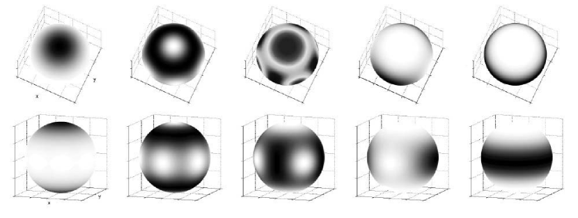
Figure 3: $Q(\theta,\varphi)$ representation of five states seen from the “north-pole” (top) and from the equatorial direction (bottom). $Q=1$ appears as black, while $Q=0$ appears as white. The five states (unnormalized) from left to right are $\left|j=4,m=4\right>+\left|j=4,m=-4\right>$, $\left|j=4,m=3\right>+\left|j=4,m=-3\right>$, $\left|j=4,m=2\right>+\left|j=4,m=-2\right>$, $\left|j=4,m=1\right>+\left|j=4,m=-1\right>$ and $\left|j=4,m=0\right>$.

Figure 3 shows the $Q(\theta,\varphi)$ representation of the following states:

• $\frac{1}{\sqrt{2}}(\left|j=4,m=4\right>+\left|j=4,m=-4\right>)$,

• $\frac{1}{\sqrt{2}}(\left|j=4,m=3\right>+\left|j=4,m=-3\right>)$,

• $\frac{1}{\sqrt{2}}(\left|j=4,m=2\right>+\left|j=4,m=-2\right>)$,

• $\frac{1}{\sqrt{2}}(\left|j=4,m=1\right>+\left|j=4,m=-1\right>)$, and

• $\left|j=4,m=0\right>$.

We see a non-classical oscillation in the x-y plane due to interference between the superposed symmetric states. As the difference between $m$ values of the components increases, the number of oscillations increases as well. As discussed in Sec. II.2.3, the states with rapid oscillations, and thus widely separated $m$ values, are particularly suspectable to $T_{2}$ relaxation. In this fashion, the structure of the $Q$-function provides a measure of the collective transverse relaxation rate.

II.3.3 Spin coherent states for all $j$ manifolds

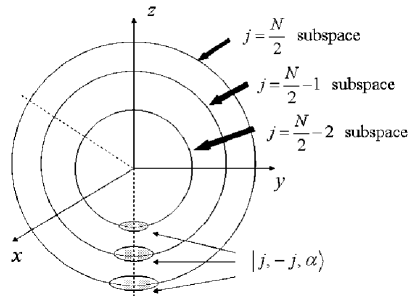
Figure 2: Spin coherent states for arbitrary $j$ manifolds.

So far, we have discussed spin coherent states for the completely symmetric subspace $(j=n/2)$ through Eq. (19). We can define spin coherent states for arbitrary values of $(0\leq j\leq n/2-1)$ by applying the rotation operator $\hat{R}_{\theta,\varphi}$ to the subradiant states $\left|j<n/2,m=-j,\alpha\right>$ Schwinger (1965). In this way, the Hilbert space can be partitioned into separate spheres with different radii $j$, as shown in Fig. 2.

III Application to selected quantum algorithms

In the previous section, we introduced three basis sets to aid in characterizing the decoherence during the execution of representative quantum algorithms. Instances of two quantum algorithms will be analyzed: the Deutsch-Jozsa algorithm Deutsch and Jozsa (1992) and Grover’s data search algorithm Grover (1997).

III.1 Deutsch-Josza algorithm

III.1.1 Standard implementation

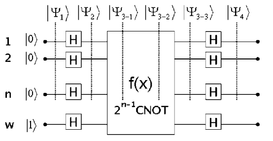
Figure 4: Circuit for the Deutsch-Jozsa algorithm.

The Deutsch-Jozsa algorithm consists of the following four steps as shown in Fig. 4.

Step1

: Preparation of an $n$-qubit control register and a one-qubit work register.

$$|\psi_{1}\rangle=|0\rangle_{c}\otimes|1\rangle_{w}$$

Step2

: Hadamard transformation.

$$\underrightarrow{\ \ \ \widehat{H}\ \ \ }\ \ \ |\psi_{2}\rangle=\frac{1}{\sqrt{2^{n}}}\sum^{2^{n}-1}_{x=0}|x\rangle_{c}\otimes\frac{1}{\sqrt{2}}(|0\rangle_{w}-|1\rangle_{w})$$

Step3

: $f$-controlled-NOT gate operation.

$$\underrightarrow{\ \ \widehat{U}_{fcN}\ \ }\ |\psi_{3}\rangle=\frac{1}{\sqrt{2^{n}}}\sum^{2^{n}-1}_{x=0}(-1)^{f(x)}|x\rangle_{c}\otimes\frac{1}{\sqrt{2}}(|0\rangle_{w}-|1\rangle_{w})$$

Step4

: Hadamard transformation.

$$\underrightarrow{\ \ \widehat{H}\ \ \ }\ \ |\psi_{4}\rangle=\frac{1}{2^{n}}\sum^{2^{n}-1}_{y=0}\sum^{2^{n}-1}_{x=0}(-1)^{f(x)+x\cdot y}|y\rangle_{c}\otimes|1\rangle_{w}$$

The $f$-controlled-NOT gate operation could be performed by expressing $f(x)$ in disjunctive-normal form and adding CNOT gates with multiple control bits for each expression. For example, consider a balanced function $f(x)$ that acts on $n=8$ qubits, yielding one if the parity of $x$ is odd and zero otherwise; let $x_{n-1},x_{n-2},\ldots,x_{0}$ be the binary digits of $x$. Let $\bar{x}_{i}$ represent the logical complement of $x_{i}$; the symbols $\vee$ and $\wedge$ are logical OR and AND, respectively. The function $f(x)$ can be expressed as

$$f(x)=\left(x_{1}\wedge x_{2}\wedge x_{3}\wedge x_{4}\wedge\bar{x}_{5}\wedge\bar{x}_{6}\wedge\bar{x}_{7}\wedge\bar{x}_{8}\right)$$

$$\vee\left(x_{1}\wedge x_{2}\wedge x_{3}\wedge\bar{x}_{4}\wedge x_{5}\wedge\bar{x}_{6}\wedge\bar{x}_{7}\wedge\bar{x}_{8}\right)\vee\ldots$$ (27)

Clearly, there will be 128 bracketed expressions for any balanced function with $n=8$. Each expression can be computed in sequence in a quantum circuit by flipping the complemented bits, performing a CNOT gate with all $n$ qubits as control bits and the work qubit as the target, and again flipping the complemented bits. Here, we consider each of these 128 blocks as a single computational step; along with the Hadamard transformations, this leads to a total of 131 steps in the algorithm, including the initial state.

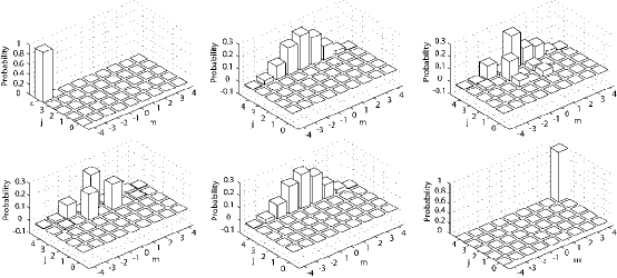
Figure 5: Projections $P(j,m)$ onto the symmetrized states for the Deutsch-Jozsa algorithm; $n=8$ and $f(x)$ is one iff the parity of $x$ is odd. The plots, proceeding left-to-right in the first and second rows, correspond to the projections of $\left|\psi_{1}\right>$ (top left) through $\left|\psi_{4}\right>$ (bottom right), indicated in Fig. 4. Note that the initial and final states for this example are $\left|\psi_{1}\right>=\left|0\right>$ and $\left|\psi_{4}\right>=\left|2^{n}-1\right>$.

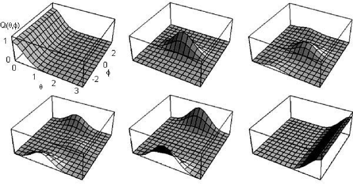
Figure 6: $Q(\theta,\varphi)$ for the Deutsch-Jozsa algorithm; the plots correspond to the states described in Fig. 5. Note that in each graph, the unit sphere has been mapped onto the $x$-$y$ plane; the transverse axes vary between $0\leq\theta\leq\pi$ and $-\pi\leq\varphi\leq\pi$.

For the $f(x)$ described above, we have calculated the projection of the state after each of these 131 steps onto the symmetric state basis; here, we only show in Fig. 5 the projections at the selected steps indicated in Fig. 4. The normalized relaxation rates can then be calculated at these instants from the projections. In Fig. 6, the projections onto the spin-coherent states is shown. The initial state $|\psi_{1}\rangle$ has $P(j,m)=\delta_{j,4}\delta_{m,-4}$ , which is transformed to a spin coherent state $\left|\psi_{2}\right>=\left|\theta=\frac{\pi}{2},\varphi=0\right>$ by Hadamard transformation. This spin coherent state has nonzero $P(j,m)$ values only in the $j=n/2$ subspace and is peaked at $m=0$, so that the state is vulnerable to superradiant decay. After implementation of half of the $f$-controlled-NOT gates ($\left|\psi_{3-2}\right>$), the $Q$-function exhibits a macroscopically-separated linear superposition, as shown in Fig. 6. The state $|\psi_{3-3}\rangle$ immediately before the second Hadamard transformation is again a spin coherent state with an opposite phase $\left|\theta=\pi/2,\varphi=\pi\right>$ compared to the state $\left|\psi_{2}\right>$.

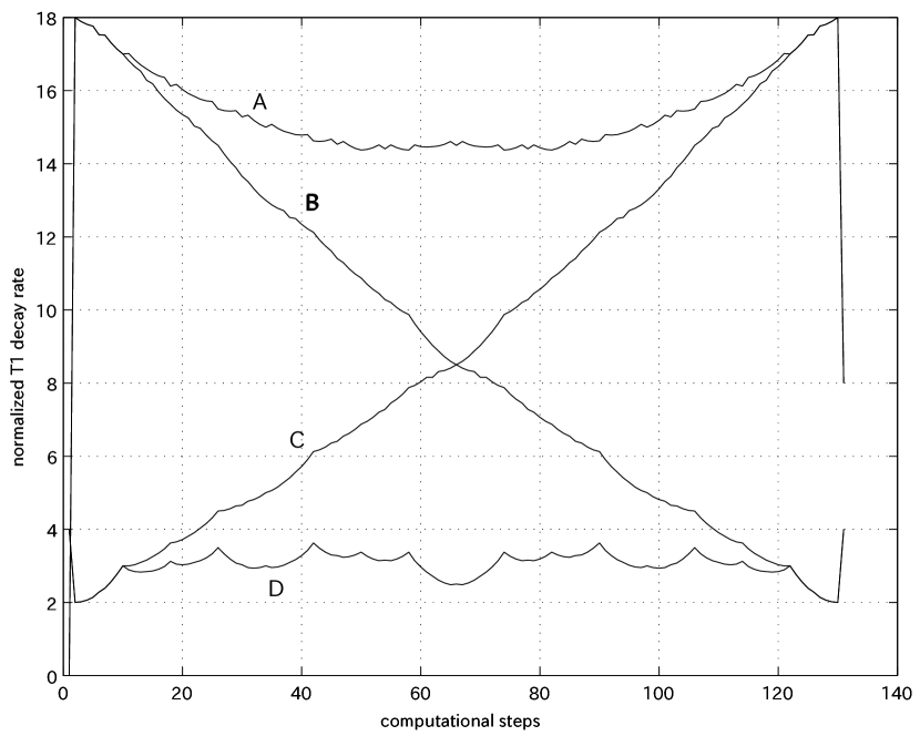
Figure 7: The normalized $T_{1}$ relaxation rates at each of the 131 computational steps in the Deutsch-Jozsa algorithm. The traces correspond to: (A) Unmodified algorithm, $f(x)=1$ if the parity of $x$ is even. (B) Unmodified algorithm, $f(x)=1$ if the parity of the last four bits of $x$ is even. (C) Improved algorithm, $f(x)$ as in A. (D) Improved algorithm, $f(x)$ as in B.

Figure 7A shows the evolution of the normalized $T_{1}$ relaxation rate at each of the 131 computational steps in the implementation of this algorithm. The $T_{1}$ relaxation rate is highest immediately after the first Hadamard gate and immediately before the second Hadamard gate, where the corresponding states $|\psi_{2}\rangle$ and $|\psi_{3-3}\rangle$ are spin-coherent states with a superradiant relaxation rate $\gamma/\gamma_{0}=18$. This relaxation rate should be compared to the overall $T_{1}$ relaxation rate $\gamma/\gamma_{0}=4$ for the case that $n=8$ spins are in the same spin-coherent state but interact individually with an external reservoir.

The normalized $T_{2}$ relaxation rate in the implementation of this algorithm jumps from zero for the ground state to ${\gamma}/{\gamma_{0}}\simeq 1.51$ for the spin-coherent state, and stays at the same rate for the remaining steps; this is due to the fact that the 128 $n$-control-bit CNOT gates used to implement $(-1)^{f(x)}$ only cause phase shifts, and do not alter the probabilities $P_{m_{1}m_{2}\dotsm m_{n}}$. Indeed, all functions $f(x)$ lead to the same $T_{2}$ relaxation rate in the intermediate 129 steps of the algorithm. This $T_{2}$ relaxation rate should be compared to the overall $T_{2}$ relaxation rate ${\gamma}/{\gamma_{0}}=4$ for the case that the $n=8$ spins are in the same spin coherent state but interact individually with an external reservoir. Note that a macroscopically separated linear superposition state $\frac{1}{\sqrt{2}}(|++\dotsm+\rangle+|--\dotsm-\rangle)$ has the same collective relaxation rate ${\gamma}/{\gamma_{0}}=4$.

One may infer that the Deutsch-Jozsa algorithm for this particular $f(x)$ function is vulnerable to collective $T_{1}$ relaxation processes, but is rather robust against collective $T_{2}$ relaxation processes.

Next, let us consider a different $f(x)$ that takes value one when the last four qubits are of odd parity, and zero otherwise. In this case, the final state of the algorithm is $\left|\psi_{4}\right>=|++++----\rangle$.

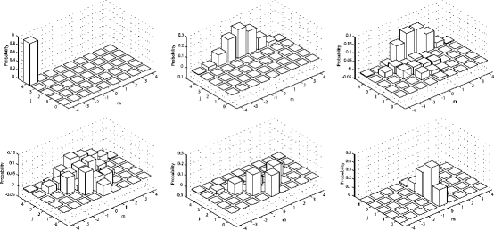
Figure 8: $P(j,m)$ for states $\left|\psi_{1}\right>$ through $\left|\psi_{4}\right>$ in Deutsch-Jozsa algorithm, $n=8$, $f(x)$ equalling one if the parity of the last four qubits is odd. Note that the initial and final state are $\left|\psi_{1}\right>=\left|0\right>$ and $\left|\psi_{4}\right>=\left|15\right>$.

Figure 8 shows the evolution of $P(j,m)$ of the $n=8$ qubit control register state. Even though the state $|\psi_{2}\rangle$ immediately after the first Hadamard transform is still subject to superradiant decay, the state $|\psi_{3-3}\rangle$ immediately before the second Hadamard transform and the final state $|\psi_{4}\rangle$ have a large support on more stable subradiant states $|j\leq n/2,m=-j\rangle$.The decreased $T_{1}$ relaxation rate for this case, compared to the previous case, is obvious in Fig. 7B.

III.1.2 Improved implementation

It is suggestive from the above examples that balanced functions $f(x)$ which result in final states with $m\simeq 0$ have rather stable $|\psi_{3}\rangle$ and $|\psi_{4}\rangle$ states against collective $T_{1}$ and $T_{2}$ processes. Therefore, external longitudinal and transverse relaxation occurs primarily after the first Hadamard transformation.

This problem can be resolved by starting the Deutsch-Jozsa algorithm with a state which has half up-spins and half down-spins. For instance, consider the initial state $|----++++\rangle$ for the $n=8$ case. This choice of the initial state does not change the fundamental structure of Deutsch-Jozsa algorithm at all; if the final state is found to be identical to the initial state, $f(x)$ is a constant function. However, the modified initial state leads to a dramatic improvement in the $T_{1}$ relaxation rate, as shown in Fig. 7C,D.

III.2 Grover’s data search algorithm

III.2.1 Standard implementation

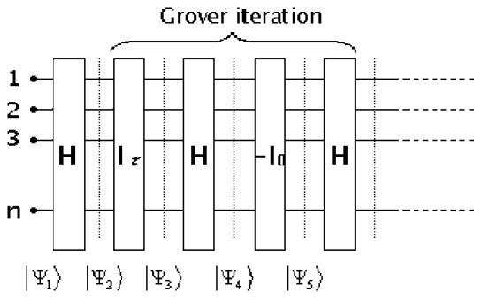
Figure 9: Circuit topology for Grover’s database search algorithm

One application of the Grover iterant in the database search algorithm consists of the following four steps, as shown in Fig. 9 Grover (1997).

Step1

: Initialization of $n$ qubit control register.

$$|\psi_{1}\rangle=|0\rangle=|---\dotsm-\rangle$$

Step2

: Hadamard transformation.

$$\underrightarrow{\ \ \ \widehat{H}\ \ \ }\ \ \ |\psi_{2}\rangle=\widehat{H}|0\rangle=\frac{1}{\sqrt{2^{n}}}\sum^{2^{n}-1}_{x=0}|x\rangle$$

Step3

: Phase flip of the target state $|\tau\rangle$.

$$\underrightarrow{\ \ \ \ \widehat{I}_{\tau}\ \ \ \ }\ \ \ |\psi_{3}\rangle=(\widehat{I}-2|\tau\rangle\langle\tau|)\widehat{H}|0\rangle\hskip 30.0pt$$

Step4

: Hadamard transform.

$$\underrightarrow{\ \ \widehat{H}\ \ \ }\ \ |\psi_{4}\rangle=\widehat{H}(\widehat{I}-2|\tau\rangle\langle\tau|)\widehat{H}|0\rangle$$

Step5

: Phase flip of the $|0\rangle$ component.

$$\underrightarrow{\ \ \ \ \widehat{I}_{0}\ \ \ }\ \ \ |\psi_{5}\rangle=-(\widehat{I}-2|0\rangle\langle 0|)\widehat{H}(\widehat{I}-2|\tau\rangle\langle\tau|)\widehat{H}|0\rangle$$

Defining the iterant $\widehat{Q}$ as $-\widehat{I}_{0}\widehat{H}\widehat{I}_{\tau}\widehat{H}$, the state $|\psi_{5}\rangle$ can be rewritten as

$$|\psi_{5}\rangle = \widehat{Q}|\psi_{1}\rangle$$ (28)

$$= -(\widehat{I}-2|0\rangle\langle 0|){\widehat{H}}^{2}|0\rangle+2(\widehat{I}-2|0\rangle\langle 0|)\widehat{H}|\tau\rangle\langle\tau|\widehat{H}|0\rangle$$

$$= (1-4|U_{\tau_{0}}|^{2})|0\rangle+2U_{\tau_{0}}\widehat{H}|\tau\rangle,$$

where $U_{\tau 0}=\langle\tau|\widehat{H}|0\rangle$.

The same rotation operator $\widehat{Q}$ translates the state $\widehat{H}|\tau\rangle$ to

$$\widehat{Q}\widehat{H}|\tau\rangle = -\widehat{I_{0}}\widehat{H}\widehat{I_{\tau}}\widehat{H}\widehat{H}|\tau\rangle$$ (29)

$$= (\widehat{I}-2|0\rangle\langle 0|)\widehat{H}|\tau\rangle$$

$$= \widehat{H}|\tau\rangle-2U_{\tau_{0}}^{\ast}|0\rangle.$$

It is clear from Eqs. (28) and (29) that the rotation operator $\widehat{Q}$ preserves the two-dimensional vector space spanned by $|0\rangle$ and $\widehat{H}|\tau\rangle$. The operator $\widehat{Q}$ rotates any linear superposition of $|0\rangle$ and $\widehat{H}|\tau\rangle$ by an angle $\theta\simeq 2|U_{\tau_{0}}|$ in this plane. The number of iterations that are required to transform an initial state $|0\rangle$ to a target state $\widehat{H}|\tau\rangle$ is therefore given by

$$l_{tot}\approx\frac{({{\pi}/{2}})}{\theta}=\frac{\pi}{4}\sqrt{2^{n}},$$ (30)

where $|U_{\tau_{0}}|=1\sqrt{2^{n}}$ is used. The target state is obtained with near unity probability by the Hadamard transformation of the final state, $\widehat{H}(\widehat{H}|\tau\rangle)=|\tau\rangle$.

Each iterant can be split into the phase flip operation of the target state $\widehat{I}_{\tau}$ and the inversion-about-the-average-probability-amplitude operation $-\widehat{H}\widehat{I}_{0}\widehat{H}$ Grover (1997). We will examine the system states after the inversion operation for the $l^{\text{th}}$ iterant.

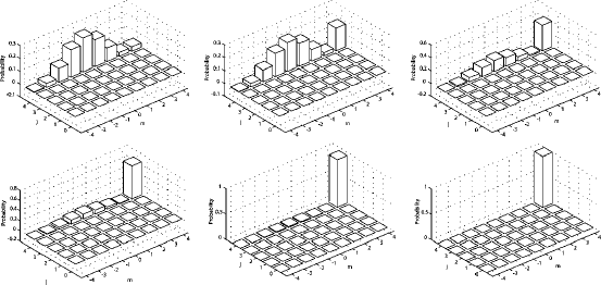
Figure 10: $P(j,m)$ of the control register states in the $n=8$ database search algorithm. The plots correspond to the states after Grover iteration $\ell\in\{1,3,5,7,10,12\}$; $\ell=1$ is top left and $\ell=12$ is bottom-right. The initial and final states are $|\psi_{1}\rangle=|0\rangle$ and $|\psi_{4}\rangle=|2^{n}-1\rangle$.

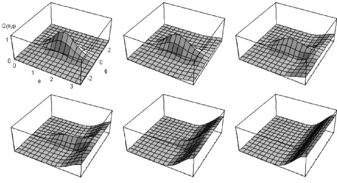
Figure 11: $Q(\theta,\varphi)$ of the control register states in the $n=8$ database search algorithm. The plots correspond to the states after Grover iteration $\ell\in\{1,3,5,7,10,12\}$; $\ell=1$ is top left and $\ell=12$ is bottom-right.

Fig. 10 shows $P(j,m)$ for $n=8$ after $l=1,3,5,7,10$ and $12$ iterations, for the case of $|\tau\rangle=|255\rangle=|++++++++\rangle$. Fig. 11 plots $Q(\theta,\varphi)$ for the same states. As expected, both plots of $P(j,m)$ and $Q(\theta,\varphi)$ indicate a monotonic decrease in the probability of finding the initial state $\widehat{H}|0\rangle$ and a monotonic increase in the probability of finding the target state. In this example, both the initial state $\widehat{H}|0\rangle$ and the target state $|\tau\rangle$ are in the completely symmetric ($j=n/2$) subspace, and so are all the intermediate states belong to this subspace. Therefore, one would expect that the implementation of the Grover algorithm for this target state is vulnerable to a collective longitudinal relaxation process.

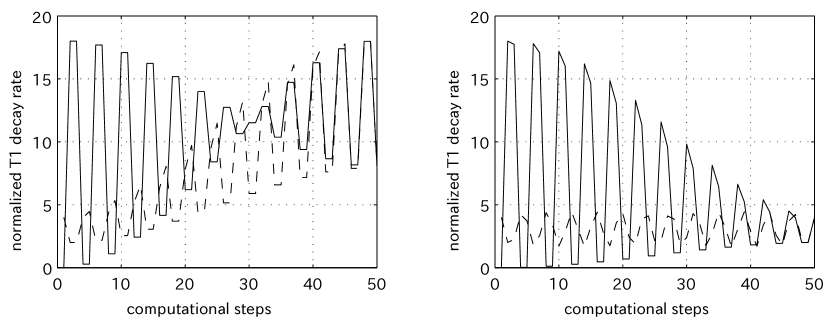
Figure 12: The normalized $T_{1}$ relaxation rates at each of the 50 computational steps for the $n=8$ database search example; the left figure applies to the target state $\left|\tau=255\right>$ and the right figure is for $\left|\tau=15\right>$. The first Hadamard gate is followed by twelve Grover iterations consisting of four steps of $-\hat{H}\hat{I}_{0}\hat{H}\hat{I}_{\tau}$. The solid and dashed lines represent results for the standard implementation using an initial state $|\psi_{1}\rangle=|0\rangle$ and the improved implementation using an initial state $|\psi_{1}\rangle=|15\rangle=|----++++\rangle$, respectively.

The solid line in the left panel of Fig. 12 shows the normalized $T_{1}$ relaxation rate at each of 50 selected evolution times, corresponding to the initial and final states, and the state after each gate in the 12 iterants. The $T_{1}$ relaxation rate is highest immediately after the first Hadamard gate and slowest immediately after the second Hadamard gate. The oscillatory behavior per iteration continues to the midpoint ($l=6$ Grover iterations in this case). The high $T_{1}$ relaxation rate corresponds to the state close to $\widehat{H}|0\rangle$ and the low $T_{1}$ relaxation rate corresponds to the state close to $|0\rangle$. At the mid-point, the phase of this oscillation is flipped. The high $T_{1}$ relaxation rate now corresponds to the state close to $\widehat{H}|\tau=255\rangle$ and the low $T_{1}$ relaxation rate corresponds to the state close to $|255\rangle$.

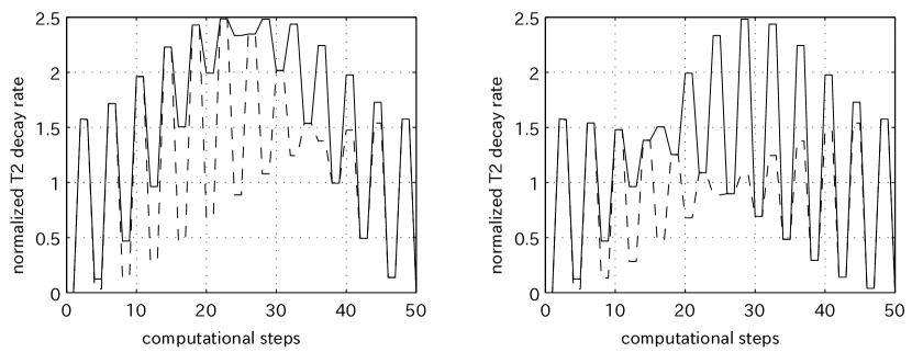
Figure 13: The normalized $T_{2}$ relaxation rates for the $n=8$ search algorithm; plots are labeled as in Fig. 12.

In the left panel of Fig. 13, the solid line indicates the normalized $T_{2}$ relaxation rate at the same 50 computational steps. The relaxation rate is increased after the first Hadamard gate since that state $\widehat{H}|0\rangle$ has a fairly large dispersion on the quantum number $m$, but is decreased after the second Hadamard gate, where the state is approximately $\sim|0\rangle-\frac{1}{8}\widehat{H}|255\rangle$ (unnormalized) which has a much smaller dispersion on $m$. The $T_{2}$ relaxation rate is further increased immediately after the third Hadamard gate, where the state is approximately $\sim\widehat{H}|0\rangle+\frac{1}{8}|255\rangle$. The $T_{2}$ relaxation rate is high again immediately before the last Hadamard gate, where the state is approximately $\sim\widehat{H}|255\rangle$ which has the same dispersion on $m$ as the state $\widehat{H}|0\rangle$, and is low again immediately before the second last Hadamard gate, where the state is approximately $\sim\frac{1}{8}\widehat{H}|0\rangle+|255\rangle$.

Evidently, this implementation of the search algorithm is vulnerable to both longitudinal and transverse relaxation processes.

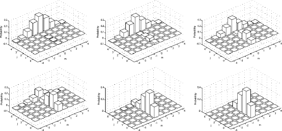
Figure 14: $P(j,m)$ of the control register states for the second $n=8$ example of the database search algorithm. The initial and final states are $|\psi_{1}\rangle=|0\rangle$ and $|\psi_{4}\rangle=|15\rangle$.

In Fig. 14, $P(j,m)$ for $n=8$ after $l=1,3,5,7,10$ and $12$ iterations is plotted for a different instance of the search algorithm, where $|\tau\rangle=|15\rangle=|----++++\rangle$ is the target state. As shown in the last panel , the target state $|\tau\rangle$ in this case has support largely in the subspaces where $j\in\{2,1,0\}$. The state transforms from an unstable superradiant state to a more stable subradiant state as the number of Grover iteration increases. The solid lines in the right panels of Figs. 12 and 13 present the calculated $T_{1}$ and $T_{2}$ relaxation rates for this instance.

III.2.2 Improved implementation

The vulnerability of the Grover algorithm implementation to collective longitudinal and transverse relaxation processes stems from the initial spin-coherent state $\widehat{H}|0\rangle$. In order to circumvent this weakness, we can start with an alternative initial state such as $|\gamma=15\rangle=|----++++\rangle$. If we replace a standard Grover iteration shown above with

$$\widehat{Q}=-(\widehat{I}-2|\gamma\rangle\langle\gamma|)\widehat{H}(\widehat{I}-2|\tau\rangle\langle\tau|)\widehat{H}\ ,$$ (31)

this new rotation operator preserves the two dimensional vector space spanned by $|\gamma\rangle$ and $\widehat{H}|\tau\rangle$. $U_{\tau_{\gamma}}=\langle\tau|\widehat{H}|\gamma\rangle$ is equal to $1/\sqrt{2^{n}}$ or $-1\sqrt{2^{n}}$, depending on $|\gamma\rangle$ and $|\tau\rangle$. The plus and minus signs correspond to the opposite rotation directions of the initial vector by a Grover iteration. Here an absolute rotation angle $\theta\simeq 2|U_{\tau_{\gamma}}|\equiv 2|\langle\tau|\widehat{H}\gamma\rangle|$ is identical to the previous rotation angle $2U_{\tau_{0}}=2\langle\tau|\widehat{H}|0\rangle$. Therefore, the $\sim\sqrt{2^{n}}$ successive operations of $\widehat{Q}$ rotates an initial state $|\gamma\rangle$ to the final state $\widehat{H}|\tau\rangle$, from which we can find the target state $|\tau\rangle$ by a single Hadamard transformation. In this way we can avoid the unstable spin coherent state $\widehat{H}|0\rangle$ from the implementation of Grover’s algorithm simply by using any computational basis state with $m=0$ as an initial state.

The improved $T_{1}$ and $T_{2}$ relaxation performance by this choice of an initial state is demonstrated by the dashed lines in Fig. 12 and 13.

IV Conclusion

We have studied the collective decoherence properties of $n$ qubit quantum registers under implementation of selected quantum algorithms. A perturbative treatment of longitudinal relaxation implies that it is preferable to modify quantum algorithms to maximize the evolution time spent in the vicinity of subradiant states $|j,m=-j\rangle$, and avoid unstable superradiant states. Here, we have shown that slight modifications of the initial states of the Deutsch-Jozsa and quantum search algorithms are advantageous in weighting more heavily the subradiant states, if error correcting codes or more complicated logical encoding is prohibitive due to limited resources. Ideally, one might use the $T_{1}$ transition rate as a parameter to optimize the gate decompositions and initial states used to implement a given algorithm. The optimal strategy whereby this can be done remains an open question.

In our approach, the transition rates were calculated only at selected discrete evolution times in each algorithm. In a forthcoming paper, we will present a finer grain analysis of the transition rates, where the algorithm is described in terms of single and two-qubit gates, and the state between each gate is considered in the overall transition rates. In addition, an argument will be espoused as to how such an analysis can approximate a continuous average over the evolution generated by a time-dependent Hamiltonian consisting of pairwise interactions and external single-qubit pulses.

The work of S.U. is partially supported by CREST, JST and that of C.P.M. and Y.Y is partially supported by NTT Basic Research Laboratories, SORST, JST and AFOSR under the contract of F49620-01-1-0556-P003-4.

Appendix A Clebsch-Gordan coefficients

$$\ \ \ \ \ \ \left[\begin{array}[]{c|c|c|c||c}\hline\cr\ \ \frac{3}{2}&\ \ \ \frac{3}{2}\ \ \ \ \ \frac{1}{2}\ \ \ \ \ \frac{1}{2}&\ \ \ \frac{3}{2}\ \ \ \ \ \frac{1}{2}\ \ \ \ \ \frac{1}{2}&\ \ \frac{3}{2}&j\\ \hline\cr\ \ \frac{3}{2}&\ \ \ \frac{3}{2}\ \ \ \ \ \frac{1}{2}\ \ \ \ \ \frac{1}{2}&-\frac{3}{2}\ -\frac{1}{2}\ -\frac{1}{2}&\ -\frac{3}{2}&m\\ \hline\cr\end{array}\right]\ \ \ \ \ \ \ \ \ \$$

$$\widehat{U}=\left[\begin{array}[]{c|ccc|ccc|c}\ \ 1&&&&&&&\\ \hline\cr&\frac{1}{\sqrt{3}}&-\frac{1}{\sqrt{6}}&\frac{1}{\sqrt{2}}&&&&\\ &\frac{1}{\sqrt{3}}&-\frac{1}{\sqrt{6}}&-\frac{1}{\sqrt{2}}&&&&\\ &\frac{1}{\sqrt{3}}&\frac{2}{\sqrt{6}}&0&&&&\\ \hline\cr&&&&\frac{1}{\sqrt{3}}&-\frac{1}{\sqrt{6}}&\frac{1}{\sqrt{2}}&\\ &&&&\frac{1}{\sqrt{3}}&-\frac{1}{\sqrt{6}}&-\frac{1}{\sqrt{2}}&\\ &&&&\frac{1}{\sqrt{3}}&\frac{2}{\sqrt{6}}&0&\\ \hline\cr&&&&&&&\ \ 1\\ \end{array}\right]\begin{array}[]{c}|+++\rangle\\ \hline\cr|++-\rangle\\ |+-+\rangle\\ |-++\rangle\\ \hline\cr|+--\rangle\\ |-+-\rangle\\ |--+\rangle\\ \hline\cr|---\rangle\\ \end{array}$$ (49)

Table 1: A diagonalizing matrix $\widehat{U}$ defined by (52) for the $n=3$ spin case. The Clebsch-Gordan coefficients for $(j,m)=(\frac{1}{2},-\frac{1}{2})$ states represent the subradiant states.

Since a symmetrized spin state $|j,m,\alpha\rangle$ satisfies the eigenvalue relations in Eq.(6) and the orthonormality relation, $\langle j^{\prime},m^{\prime},\alpha^{\prime}|j,m,\alpha\rangle=\delta_{jj^{\prime}}\delta_{mm^{\prime}}\delta_{\alpha\alpha^{\prime}}$, the squared total angular momentum $\widehat{J}^{2}$ is a diagonal matrix in this basis:

$$\langle j^{\prime},m^{\prime},\alpha^{\prime}|\widehat{J}^{2}|j,m,\alpha\rangle=j(j+1)\delta_{jj^{\prime}}\delta_{mm^{\prime}}\delta_{\alpha\alpha^{\prime}}.$$ (50)

By inserting two identity operators $\widehat{I}=\sum_{m_{1}\dotsi m_{n}}|m_{1}m_{2}\dotsi m_{n}\rangle\langle m_{1}m_{2}\dotsi m_{n}|$ before and after $\widehat{J}^{2}$ in the above equation, we obtain

$$\sum_{m_{1}^{\prime}\dotsi m_{n}^{\prime}}\sum_{m_{1}\dotsi m_{n}}\langle j^{\prime},m^{\prime},\alpha^{\prime}|m_{1}^{\prime},m_{2}^{\prime},\dotsi,m_{n}^{\prime}\rangle$$

$$\langle m_{1}^{\prime},m_{2}^{\prime},\dotsi,m_{n}^{\prime}|\widehat{J}^{2}|m_{1},m_{2},\dotsi,m_{n}\rangle$$

$$\langle m_{1},m_{2},\dotsi,m_{n}|j,m,\alpha\rangle=j(j+1)\delta_{jj^{\prime}}\delta_{mm^{\prime}}\delta_{\alpha\alpha^{\prime}}\ .$$ (51)

This equation suggests that the non-diagonal matrix $\langle m_{1}^{\prime},m_{2}^{\prime},\dotsi,m^{\prime}_{N}|\widehat{J}^{2}|m_{1},m_{2},\dotsi,m_{N}\rangle$ can be transformed into the diagonal matrix $\langle j^{\prime},m^{\prime},\alpha^{\prime}|\widehat{J}^{2}|j,m,\alpha\rangle$ with eigenvalues $j(j+1)$ by multiplying a unitary matrix $\widehat{U}$ and its inverse $\widehat{U}^{-1}$ from right and left of the non-diagonal matrix, where

$$\widehat{U}=\sum_{m_{1},\dotsi,m_{N}}\langle m_{1},m_{2},\dotsi m_{N}|j,m,\alpha\rangle.$$ (52)

Each column of this real unitary matrix provides the probability amplitude $c_{m_{1},\dotsi,m_{n}}$ for linear expansion of $|j,m,\alpha\rangle$ in terms of $|m_{1},m_{2},\dotsi,m_{n}\rangle.$, i.e.

$$|j,m,\alpha\rangle=\sum_{m_{1}\dotsi m_{n}}c_{m_{1}\dotsi m_{n}}|m_{1},m_{2},\dotsi m_{n}\rangle.$$ (53)

The coefficients $c_{m_{1},\dotsi,m_{n}}$ are the Clebsch-Gordan coefficients r_j .

According to the above argument, the symmetrized states $|j,m,\alpha\rangle$ are mathematically constructed by the following procedure.

1. Divide computational basis states into the groups with different total longitudinal quantum number $m=\sum^{n}_{i=1}m_{i};$ For instance, $n=3$ spin states are split into four subspaces $m=-\frac{3}{2},-\frac{1}{2},\frac{1}{2},\frac{3}{2}$ as shown in the right column in Table 1.

2. Calculate $\widehat{J}^{2}$ in terms of computational basis states. Here, non-zero elements appear only in block diagonal sub-matrices belonging to the same subspace designated by $m$.

3. Find the real unitary matrix $\widehat{U}$ which diagonalizes $\widehat{J}^{2}$, where the diagonal elements of the diagonalized matrix are identically equal to the eigenvalue $j(j+1)$.

4. The probability amplitudes of computational basis states for constructing each symmetrized state (Clebsch-Gordan coefficients) are given by each column of the real unitary matrix $\widehat{U}$. The example for $n=4$ is listed in the left part of Table 1.

The $n$-spin symmetrized states are grouped into different subspaces by their eigenvalues $j$ and $m$ as shown in Table 2. The first column with $j=\frac{n}{2}$ represents a set of completely symmetric states, which is often referred to as angular momentum eigenstates. These states have no degeneracy, so the total number of the completely symmetric states is $n+1$, corresponding to $m=\frac{n}{2},\frac{n}{2}-1,\dotsi,-\frac{n}{2}+1,-\frac{n}{2}$. The second column with $j=\frac{n}{2}-1$ and $m=\frac{n}{2}-1,\dotsi,-\frac{n}{2}+1$ represents $d={}_{n}C_{1}-{}_{n}C_{0}=(n-1)th$ fold degenerate states. The total number of eigenstates in this subspace is $(n-1)\times(n-1)=(n-1)^{2}$. The third column with $j=\frac{n}{2}-2$ and $m=\frac{n}{2}-2,\ \dotsi,-\frac{n}{2}+2$ represents $d={}_{n}C_{2}-{}_{n}C_{1}=\frac{n}{2}(n-3)th$ fold degenerate states. The total number of eigenstates in this subspace is $(n-3)\times\frac{n}{2}(n-3)=\frac{n}{2}(n-3)^{2}$ The final $j$ manifold ends with either $j=\frac{1}{2}$ (if $n$ is an odd number) or $j=0$ (if $n$ is an even number). In general the degeneracy of the states $|j,m\rangle$ is given by Dicke (1954),

$$\frac{n!(2j+1)}{(\frac{n}{2}+j+1)!(\frac{n}{2}-j)!}\ ,$$ (54)

which is independent of $m$.

$$\begin{array}[]{ccc|cccc}&&&j=\frac{N}{2}&j=\frac{N}{2}-1&j=\frac{N}{2}-2&\dotsi\\ &&&(d=1)&(d=N-1)&(d=\frac{N}{2}(N-3))&\dotsi\\ \hline\cr m&=&\frac{N}{2}&\frac{\ }{\ \ \ \ \ }&&&\\ m&=&\frac{N}{2}-1&\frac{\ }{\ \ \ \ \ }&\frac{\ }{\ \ \ \ \ }&&\\ m&=&\frac{N}{2}-2&\frac{\ }{\ \ \ \ \ }&\frac{\ }{\ \ \ \ \ }&\frac{\ }{\ \ \ \ \ }&\\ &&&\vdots&\vdots&\vdots&\dotsi\\ m&=&-\frac{N}{2}+2&\frac{\ }{\ \ \ \ \ }&\frac{\ }{\ \ \ \ \ }&\frac{\ }{\ \ \ \ \ }&\\ m&=&-\frac{N}{2}+1&\frac{\ }{\ \ \ \ \ }&\frac{\ }{\ \ \ \ \ }&&\\ m&=&-\frac{N}{2}&\frac{\ }{\ \ \ \ \ }&&&\\ \end{array}$$ (64)

Table 2: A distribution of symmetrized states $|j,m,\alpha\rangle$.

Appendix B Collective longitudinal $(T_{1})$ relaxation rate

The collective spin-reservoir interaction Hamiltonian, which is responsible for a $T_{1}$ relaxation process, is given by Eq. (1). We will solve the Schrödinger equation,

$$i\hbar\frac{d}{dt}|\psi(t)\rangle=(\widehat{\cal H}_{0}+\widehat{\cal H}_{I})|\psi(t)\rangle\ ,$$ (65)

with an initial state

$$|\psi(0)\rangle=|j,m,\alpha\rangle\otimes\Pi_{i}|0\rangle\ .$$ (66)

We assume that all bosonic modes with a continuous spectrum are in ground states at $t=0$. $\widehat{\cal H}_{0}=\hbar\omega\widehat{J}^{z}+\sum_{i}\hbar\omega_{i}\widehat{a}_{i}^{\dagger}\widehat{a}_{i}$ is a free Hamiltonian for the combined spin-boson system. A time dependent solution of the Schrödinger equation is

$$|\psi(t)\rangle=c_{m,0}(t)e^{-i\omega mt}|j,m,\alpha\rangle|0\rangle+$$

$$\sum_{i}c_{m-1,1_{i}}(t)e^{-i\omega(m-1)t-i\omega_{i}t}|j,m-1,\alpha\rangle|1_{i}\rangle\ ,$$ (67)

where $|0\rangle=\Pi_{i}|0\rangle_{i}$ and $|1_{i}\rangle=|0\rangle_{1}\dotsm|0\rangle_{i-1}|1\rangle_{i}\dotsm$.

Substituting Eq. (67) into Eq. (65), we obtain

$$i\hbar[\dot{c}_{m,0}(t)e^{-i\omega mt}|j,m,\alpha\rangle|0\rangle$$ (68)

$$+ \sum_{i}\dot{c}_{m-1,1_{i}}(t)e^{-i\omega(m-1)t-i\omega_{i}t}|j,m-1,\alpha\rangle|1_{i}\rangle$$

$$= \hbar\sum_{i}k_{i}[c_{m,0}(t)e^{i\omega mt}\sqrt{j(j+1)-m(m-1)}$$

$$\times |j,m-1,\alpha\rangle|1_{i}\rangle+c_{m-1,1_{i}}(t)e^{-i\omega(m-1)t-i\omega_{i}t}$$

$$\times \sqrt{j(j+1)-m(m-1)}|j,m,\alpha\rangle|0\rangle]\ .$$

Multiplying $\langle j,m,\alpha|\langle 0|$ and $\langle j,m,\alpha|\langle 1_{i}|$ on both sides of Eq. (68), we have the coupled mode equations for $c_{m,0}(t)$ and $c_{m-1,1_{i}}(t)$,

$$\dot{c}_{m,0}(t) = -i\sum_{i}k_{i}\sqrt{j(j+1)-m(m-1)}$$ (69)

$$\times e^{i(\omega-\omega_{i})t}c_{m-1,1_{i}}(t)\ ,$$

$$\dot{c}_{m-1,1_{i}}(t) = -ik_{i}\sqrt{j(j+1)-m(m-1)}$$ (70)

$$\times e^{i(\omega-\omega_{i})t}c_{m,0}(t)\ ,$$

The initial condition for the above equations is

$$c_{m,0}(0)=1.$$

$$c_{m-1,1_{i}}(0)=0.$$ (71)

We can integrate Eq. (70), taking initial condition Eq. (71) into account, and substitute $c_{m-1,1_{i}}(t)$ into Eq. (69) to obtain the following integro-differential equation

$$\dot{c}_{m,0}(t)=-\sum_{i}k_{i}^{2}[j(j+1)-m(m-1)]$$

$$\int_{0}^{t}dt^{\prime}e^{i(\omega-\omega_{i})(t-t^{\prime})}c_{m,0}(t^{\prime})dt^{\prime}$$ (72)

If we replace $c_{m,0}(t^{\prime})$ in the righthand side of Eq. (72) by $c_{m,0}(t)$ and replace the summation $\sum_{i}$ by an integral $\int\rho(\omega_{i})d\omega_{i}$ with an energy density of states $\rho(\omega_{i})$, (72) is reduced to Cohen-Tannoudji (1977)

$$\dot{c}_{m,0}(t)=-\frac{\gamma}{2}c_{m,0}(t)\ ,$$ (73)

where

$$\gamma=\frac{2\pi}{\hbar}k^{2}(\omega)[j(j+1)-m(m-1)]\rho(\omega)\ ,$$ (74)

where we neglect the frequency shift. Since $\gamma_{0}=\frac{2\pi}{\hbar}k^{2}\rho(\omega)$ is a longitudinal relaxation rate for a single spin, the collective relaxation rate is enhanced or suppressed by a factor of $j(j+1)-m(m-1)$.

Appendix C Collective transverse $(T_{2})$ relaxation rate

The collective spin-probe interaction Hamiltonian, by which a QND measurement of $\widehat{J}^{z}$ is realized, is given by Eq. (1). We assume the use of a single bosonic mode as a quantum probe and thus the summation over mode index $i$ is suppressed. We will solve the Schrödinger equation

$$i\hbar\frac{d}{dt}|\psi(t)\rangle=\widehat{\cal H}_{I}|\psi(t)\rangle\ ,$$ (75)

where a free Hamiltonian $\widehat{\cal H}_{0}$ is suppressed. The unitary time evolution operator in this case is reduced to

$$\widehat{U}(t)=\exp[-igt\widehat{J}^{z}\widehat{a}^{\dagger}\widehat{a}]\ .$$ (76)

We assume the initial state for the spin and probe systems is given by

$$|\psi(0)\rangle= [c_{m}|j,m,\alpha\rangle+c_{m^{\prime}}|j^{\prime},m^{\prime},\alpha^{\prime}\rangle]_{s}$$

$$\otimes\sum_{n}c_{n}|n\rangle_{p}.$$ (77)

The state after the interaction is obtained by

$$|\psi(t)\rangle = \widehat{U}(t)|\psi(0)\rangle$$

$$= \sum_{n}[c_{m}e^{igmnt}|j,m,\alpha\rangle_{s}$$

$$+ c_{m^{\prime}}e^{igm^{\prime}nt}|j^{\prime},m^{\prime},\alpha^{\prime}\rangle_{s}]\otimes c_{m}|n\rangle_{p},$$

where $\widehat{J}^{z}|j,m,\alpha\rangle$ and $\widehat{a}^{\dagger}\widehat{a}|n\rangle=n|n\rangle$ are used.

The reduced density operator $\widehat{\rho}_{s}^{(red)}$ for the spin system corresponding to Eq. (C) has the following non-zero components:

$$\widehat{\rho}_{s}^{(red)} \equiv\text{Tr}_{\rho}(|\psi\rangle\langle\psi|)$$ (79)

$$=[|c_{m}|^{2}|j,m,\alpha\rangle\langle j,m,\alpha|$$

$$\ +|c_{m^{\prime}}|^{2}|j^{\prime},m^{\prime},\alpha^{\prime}\rangle\langle j^{\prime},m^{\prime},\alpha^{\prime}|$$

$$\ +c_{m}c_{m^{\prime}}^{*}\sum_{n}|c_{n}|^{2}e^{-ig(m-m^{\prime})nt}|j,m,\alpha\rangle\langle j^{\prime},m^{\prime},\alpha^{\prime}|$$

$$\ +c_{m^{\prime}}c_{m}^{*}\sum_{n}|c_{n}|^{2}e^{-ig(m^{\prime}-m)nt}|j^{\prime},m^{\prime},\alpha^{\prime}\rangle\langle j,m,\alpha|]$$

Eq. (79) suggests that the off-diagonal element has an oscillation frequency broadening $\varDelta\omega=g|m-m^{\prime}|\langle\varDelta\widehat{n}^{2}\rangle^{1/2}$, where $\langle\varDelta\widehat{n}^{2}\rangle^{1/2}=\sum_{n}|c_{n}|^{2}(\widehat{n}-\langle\widehat{n}\rangle)^{2}$ is the variance of the particle number. If we consider this frequency broading as a continuous variable, the off-diagonal elements $c_{m}c_{m^{\prime}}^{*}$ and $c_{m^{\prime}}c_{m}^{*}$ relax with a rate given by

$$\varGamma=cg|m-m^{\prime}|\langle\varDelta\widehat{n}^{2}\rangle^{\frac{1}{2}}\ ,$$ (80)

where $c$ is a constant determined by the distribution $|c_{m}|^{2}$. For a single isolated spin in a linear superposition state where $|m-m^{\prime}|=1$, the transverse relaxation rate is $\varGamma_{0}=cg\langle\Delta\widehat{n}^{2}\rangle^{\frac{1}{2}}$. Therefore, the collective transverse relaxation rate is either or suppressed by a factor of $|m-m^{\prime}|$, compared to that of a single spin.

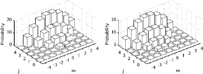
Figure 1: Normalized matrix elements for upward (left) and downward (right) transitions as a function of $j$ and $m$.

References

- Loss and DiVincenzo (1998) D. Loss and D. DiVincenzo, Phys. Rev. A 57, 120 (1998).
- Kane (1998) B. Kane, Nature 292, 133 (1998).
- Yamaguchi and Yamamoto (1998) F. Yamaguchi and Y. Yamamoto, Appl. Phys. A 57, 120 (1998).
- Ladd et al. (2002) T. Ladd, J. Goldman, F. Yamaguchi, Y. Yamamoto, E. Abe, and K. Itoh, Phys. Rev. Lett. 89, 017901 (2002).
- Slichter (1990) C. Slichter, Principles of Magnetic Resonance (Springer, New York, 1990).
- (6) A. Y. Kitaev, eprint quant-ph/9511026.
- Palma et al. (1996) G. Palma, K. Suominen, and A. Ekert, Proc. R. Soc. London, Ser. A 452, 567 (1996).
- Duan and Guo (1998) L.-M. Duan and G.-C. Guo, Phys. Rev. A 57, 737 (1998).
- Zanardi and Rasetti (1997) P. Zanardi and M. Rasetti, Phys. Rev. Lett. 79, 3306 (1997).
- Zanardi (1998) P. Zanardi, Phys. Rev. A 57, 3276 (1998).
- Lidar et al. (1998) D. Lidar, I. Chuang, and K. Whaley, Phys. Rev. Lett. 81, 2594 (1998).
- Knill et al. (2000) E. Knill, R. Laflamme, and L. Viola, Phys. Rev. Lett. 84, 2525 (2000).
- (13) D. Lidar and K. Whaley, eprint quant-ph/0301032.
- Dicke (1954) R. Dicke, Phys. Rev. 93, 99 (1954).
- Bonifacio et al. (1969) R. Bonifacio, D. Kim, and M. Scully, Phys. Rev. 187, 441 (1969).
- Arecchi et al. (1972) F. Arecchi, E. Courtens, R. Gilmore, and H. Thomas, Phys. Rev. A 6, 2211 (1972).
- Deutsch and Jozsa (1992) D. Deutsch and R. Jozsa, Proc. R. Soc. London, Ser. A 439, 553 (1992).
- Grover (1997) L. Grover, Phys. Rev. Lett. 80, 4329 (1997).
- Glauber (1963) R. Glauber, Phys. Rev. 130, 2529 (1963).
- Schwinger (1965) J. Schwinger, in Quantum Theory of Angular Momentum, edited by L. Biedenharm and H. V. Dam (Academic, 1965), p. 229.
- (21) For example, see J.J. Sakurai, Modern Quantum Mechanics, (Addison-Wesley, UK, 1993).
- Cohen-Tannoudji (1977) C. Cohen-Tannoudji, Quantum Mechanics: Vol. 2 (Wiley-Interscience, 1977).