Quantum dynamics of a model for two Josephson-coupled Bose–Einstein condensates

Abstract

In this work we investigate the quantum dynamics of a model for two single-mode Bose–Einstein condensates which are coupled via Josephson tunneling. Using direct numerical diagonalisation of the Hamiltonian, we compute the time evolution of the expectation value for the relative particle number across a wide range of couplings. Our analysis shows that the system exhibits rich and complex behaviours varying between harmonic and non-harmonic oscillations, particularly around the threshold coupling between the delocalised and self-trapping phases. We show that these behaviours are dependent on both the initial state of the system as well as regime of the coupling. In addition, a study of the dynamics for the variance of the relative particle number expectation and the entanglement for different initial states is presented in detail.

PACS: 75.10.Jm, 71.10.Fd, 03.65.Fd

1 Introduction

The phenomenon of Bose–Einstein condensation, while predicted long ago [1, 2], is nowadays responsible for many of the current perspectives on the potential applications of quantum systems. This point of view has arisen with the experimental observation of condensation in systems of ultracold dilute alkali gases, realised by several research groups using magnetic traps with various kinds of confining geometries. Reviews of the breakthroughs that have lead to the current state of development can be found in [3, 4]. These types of experimental apparatus open up the possibility for studying dynamical regimes at the frontier between the quantum and classical scenarios, where new macroscopic quantum phenomenon can emerge; for example, coherent atomic lasers [5], and the new chemistry of atomic-molecular condensates [6]. Subsequently, Bose–Einstein condensates are seen as one of the main tools to investigate, verify and improve our understanding of many concepts and principles in quantum physics, such as entanglement [7]. It is widely accepted that entanglement is the main resource needed for the implementation of quantum computation [8].

The work on ultracold atomic gases has demonstrated the occurence of Rabi oscillations due to quantum tunneling between two internal states of a condensate, similar to the Josephson effect in superconductors. Moreover, quite unexpected results were found in [9, 10], where it was shown that the temporal evolution of the expectation value of the number of particles exhibits a collapse and revival behaviour (see also e.g. [11]). This is a novel effect, not observed with spatial and temporal resolution in other systems where quantum effects take a macroscopic scale, like the superfluid and the superconducting systems.

From the theoretical point of view tunneling in Bose–Einstein condensates has been widely investigated using a simple two-mode Hamiltonian (see eq. (1) in the next section). This model has been studied by many authors using a variety of methods, such as the Gross-Pitaevskii approximation [12], mean-field theory [13, 14], quantum phase model [15], and the Bethe ansatz method [16, 17]. Our aim in this work is to expand on the theoretic knowledge of tunneling in Bose–Einstein condensates by undertaking a detailed and systematic analysis of the quantum dynamics of this two-mode Hamiltonian by means of the method of direct numerical diagonalisation. In particular, we will consider the temporal evolution of the expectation value for the relative number of particles between the two condensates for different choices of the coupling parameters and distinct initial states. In this procedure we will keep the total number of particles fixed, while the coupling of the Hamiltonian is varied. Using the numerical diagonalisation method, we are able to study the model across all coupling regimes.

We also implement this same approach to investigate the temporal evolution of entanglement for this model, and contrast this against the variance of the relative number of particles. As discussed in [18], there are generally two approaches for creating entanglement in many-body systems. One is to engineer a gapped system whose ground state is known to be entangled. By then sufficiently cooling the system to the ground state configuration, it will be entangled. In this respect there have been studies of ground state entanglement for the $XYh$ model [19, 20], the BCS model [21] and two-mode Bose-Einstein condensates including the present model [14]. Alternatively, one can manipulate a system so that a given initial state temporally evolves into an entangled state. From this point of view entanglement dynamics for coupled Bose-Einstein condensates have been investigated in [22], using the same model we study here, but with severe constraints on the choice of couplings, and also in [14]. Here we will investigate the behaviour of the entanglement evolution across different coupling regimes.

2 The model

We will study the dynamics of a model for two single-mode Bose–Einstein condensates which are coupled via Josephson tunneling. The model is not only applicable to tunneling in atomic Bose–Einstein condensates, but also mesoscopic solid state Josephson junctions [12, 15, 23] and non-linear optics [22]. The Hamiltonian is given by

$$H=\frac{k}{8}(N_{1}-N_{2})^{2}-\frac{\Delta\mu}{2}(N_{1}-N_{2})-\frac{{\cal E}_{\mathcal{J}}}{2}(a^{\dagger}_{1}a_{2}+a_{2}^{\dagger}a_{1})$$ (1)

where we follow the notational conventions of [12] for the couplings. Above, $a^{\dagger}_{i},a_{i}$ ($i=1,2$) are the creation and annihilation operators for bosons occupying one of two modes, labelled 1 and 2, and $N_{1}$ and $N_{2}$ are the respective number operators. The operator $N=N_{1}+N_{2}$ is the total boson number operator and it is conserved. The coupling $k$ provides the strength of the scattering interaction between bosons, $\Delta\mu$ is the external potential and ${\cal E}_{\mathcal{J}}$ is the coupling for the tunneling. We remark that a change of sign in the tunneling coupling ${{\cal E}_{\mathcal{J}}}\rightarrow{-{\cal E}_{\mathcal{J}}}$ is equivalent to the unitary transformation $a_{1}\rightarrow a_{1},\,a_{2}\rightarrow-a_{2}$. In that which follows we will mostly discuss the case $\Delta\mu=0$.

Let us now, for future use, distinguish different coupling regimes of the model characterised by different ratios of $k/{\cal E}_{\mathcal{J}}$. We first mention that there exists a threshold coupling $k/{\cal E}_{\mathcal{J}}=4/N$ which signifies the transition between delocalisation and self-trapping [13] (see also [18]):

• Delocalisation $\longrightarrow$ $k/{\cal E}_{\mathcal{J}}<4/N$

• Self-trapping $\longrightarrow$ $4/N<k/{\cal E}_{\mathcal{J}}$

Following [12], it is also useful to consider the following three regimes:

• Rabi regime $\longrightarrow$ $k/{\cal E}_{\mathcal{J}}<<1/N$

• Josephson regime $\longrightarrow$ $1/N<<k/{\cal E}_{\mathcal{J}}<<N$

• Fock regime $\longrightarrow$ $k/{\cal E}_{\mathcal{J}}>>N.$

For these three regimes it is known that an analogy can be drawn between the dynamics of (1) and the dynamics of certain pendulums [12]. Comparing the above classifications it is seen that the threshold coupling lies in the crossover between the Rabi and Josephson regimes, thus offering a candidate to precisely define the boundary between these regimes.

Below the quantum dynamics of (1) will be investigated using the method of direct numerical diagonalisation, which allows for a study across all couplings. It is well known that the time evolution of any physical quantity is determined through the temporal operator $U$, given by

$$U=\sum_{n=0}^{N}e^{-i\lambda_{n}t}|\psi_{n}\rangle\langle\psi_{n}|$$ (2)

where $\{\lambda_{n}\}$ and $\{|\psi_{n}\rangle\}$ are the eigenvalues and eigenvectors of the Hamiltonian (1). Therefore, the temporal evolution of any state can be calculated by

$$|\psi(t)\rangle=\sum_{n=0}^{N}a_{n}e^{-i\lambda_{n}t}|\psi_{n}\rangle,$$ (3)

where $a_{n}=\langle\psi_{n}|\phi\rangle$ and $|\phi\rangle$ represents the initial state. Using eqs. (2) and (3) we can compute the expectation value and the variance (which is a measure of the quantum fluctuations) of any physical quantity represented by a self-adjoint operator, as well as the entanglement. In particular, the temporal dependence of the expectation value of any operator $A$ can be computed using the expression

$$\langle A\rangle=\langle\psi(t)|A|\psi(t)\rangle,$$

while the variance is given by

$$\Delta(A)=\langle A^{2}\rangle-\langle A\rangle^{2}.$$

Following [24], for any pure state density matrix $\rho$ of a bipartite system the entanglement is defined by

$$E(\rho)=-{\rm tr}(\rho_{1}\log_{2}\rho_{1})=-{\rm tr}(\rho_{2}\log_{2}\rho_{2})$$

where ${\rho}_{1}$ is the reduced density matrix obtained by taking the partial trace of $\rho$ over the subsystem $2$. The definition for $\rho_{2}$ is analogous. Here we follow the approach argued in [14]. Due to indistinguishability, it is not useful to consider entanglement between individual bosons. Rather, we take the two modes of the Hamiltonian (1) to define two subsystems, which can be distinguished through the operators $N_{1}$ and $N_{2}$ representing measurement of each subsystem population. In this case, $E(\rho)$ is equivalent to [14]

$$E(\rho)=-\sum_{n=0}^{N}|c_{n}(t)|^{2}\log_{2}(|c_{n}(t)|^{2})$$

where the $c_{n}(t)$ are the co-efficients of a general state of the system

$$|\psi(t)\rangle=\sum_{n=0}^{N}c_{n}(t)|N-n,n\rangle.$$

The states $|m,n\rangle$, which collectively provide a basis for the Fock space, are given by

$$|m,n\rangle=\frac{(a_{1}^{\dagger})^{m}(a_{2}^{\dagger})^{n}}{\sqrt{m!}\sqrt{n!}}|0\rangle,$$

and $|0\rangle$ is the Fock space vacuum. For a system of $N$ total particles the maximal entanglement is $E_{\rm max}=\log_{2}(N+1)$.

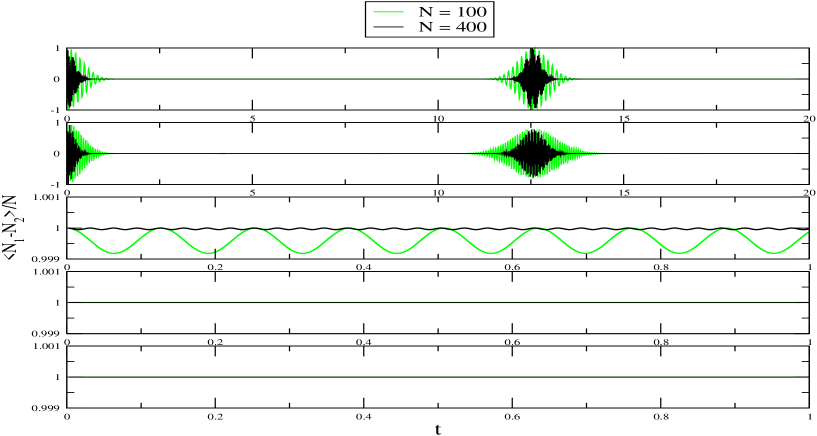
Figure 1: Time evolution of the expectation value for the relative number of particles for different ratios of the coupling $k/{\cal E}_{\mathcal{J}}$ from the top (Rabi regime) to the bottom (Fock regime): $k/{\cal E}_{\mathcal{J}}=1/N^{2},1/N,1,N,N^{2}$ for $N=100,400$ and the initial state is $|N,0\rangle$.

3 Expectation value of the relative particle number

First we investigate the quantum dynamics of the relative particle number operator $N_{1}-N_{2}$ (or the imbalance), in the three different regimes, Rabi, Josephson and Fock, as well as in the intermediate ones. For this purpose we use the expressions of the previous section together with the eigenvalues and eigenvectors obtained directly from numerical diagonalisation of the Hamiltonian (1).

From fig. 1, it is apparent that the qualitative behaviour in each region, using the same initial state, does not depend on the number of particles. (In this figure, as in the others following, the chosen time interval is one which most clearly shows the relevant dynamical behaviour.) We found that in the interval $k/{\cal E}_{\mathcal{J}}\in[1/N^{2},1/N]$ (close to the Rabi regime) the collapse and revival time takes the constant value $t_{cr}=4\pi$. Also, in the region where $k/{\cal E}_{\mathcal{J}}-1$ is small and negative, the expectation value still displays collapse and revival behaviour with harmonic oscillations occurring at the value $k/{\cal E}_{\mathcal{J}}=1$. At this coupling the period of oscillations is not independent of $N$. Still with reference to fig. 1, we observed in the region where $k/{\cal E}_{\mathcal{J}}-1$ is small and positive that the expectation value has small amplitude periodic oscillation close to the initial expectation value of $1$. The amplitude of the oscillations disappear as the ratio $k/{\cal E}_{\mathcal{J}}$ becomes larger (near the Fock regime) at which point the bosons remain localised to the subsystem of the initial configuration. However this transition from small amplitude harmonic oscillations to complete localisation appears to be smooth. Hereafter we will focus most of our attention to the Rabi and Josephson regimes, including the crossover, as this is where the most complex behaviour is to be found.

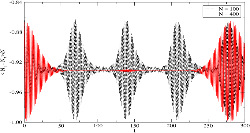
Figure 2: Time evolution for the expectation value of the relative number of particles for the initial state $|0,N\rangle$. The dot-dashed line is for $N=100$ and the solid line is for $N=400$ with ${\cal E}_{\mathcal{J}}=1$ and $k=8/N$.

In fig. 2, we plot the expectation value for the relative number of particles for two different cases: $N=100$ and $N=400$, with the initial state $|0,N\rangle$. Using the relation $k/{\cal E}_{\mathcal{J}}=8/N$ we reproduce figure 5 of [13], taking into account the different notational conventions and using a different time interval to show the collapse and revival for both cases. For this case we have followed the conventions used in [13] for the time scale by setting ${\cal E}_{\mathcal{J}}=1$ and $k=8/N$. It is apparent that under this convention the collapse and revival time is not independent of $N$. However, introducing a rescaled collapse and revival time $t_{cr}^{*}=8t_{cr}/N$, which corresponds to our adopted time scale convention, shows that $t_{cr}^{*}$ is independent of $N$. A distinguishing feature of fig. 2 is that the mean value (i.e. time-averaged value) of the imbalance is not zero, in contrast to the collapse and revival sequences shown in fig. 1. This is because the respective couplings lie in regimes on different sides of the threshold value $k/{\cal E}_{\mathcal{J}}=4/N$, and these cases respectively illustrate the behaviour associated with self-trapping and delocalisation.

In fig. 3 we can see in detail for the case $N=100$ the evolution of the dynamics from a collapse and revival sequence with $t_{cr}=4\pi$ for $k/{\cal E}_{\mathcal{J}}<4/N$, through the self-trapping transition at $k/{\cal E}_{\mathcal{J}}=4/N$, and toward small amplitude harmonic oscillations in the imbalance of the localised state when $k/{\cal E}_{\mathcal{J}}=1$. Where there is clear collapse and revival in the self-trapping phase we find that $t_{cr}$ increases with increasing $k/{\cal E_{\mathcal{J}}}$. Further increases in $k/{\cal E_{\mathcal{J}}}$ lead to a decaying of the collapse and revival sequence toward harmonic oscillations which occur at $k/{\cal E}_{\mathcal{J}}=1$.

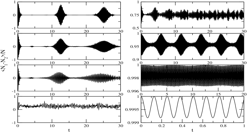
Figure 3: Time evolution of the expectation value between $k/{\cal E}_{\mathcal{J}}=1/N$ and $k/{\cal E}_{\mathcal{J}}=1$. On the left, from top to bottom $k/{\cal E}_{\mathcal{J}}=1/N,2/N,3/N,4/N$ and on the right, from top to bottom $k/{\cal E}_{\mathcal{J}}=5/N,10/N,50/N,1$, where $N=100$ and the initial state is $|N,0\rangle$.

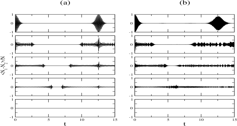
Figure 4: Relative number expectation values for (a) the Rabi regime ($k/{\cal E}_{\mathcal{J}}=1/N^{2}$); (b) between the Rabi and Josephson regimes ($k/{\cal E}_{\mathcal{J}}=1/N$). The initial states, from top to bottom are $|100,0\rangle,|90,10\rangle,|74,26\rangle,|60,40\rangle$ and $|50,50\rangle$.

Next we turn our attention to study the evolution of the expectation value $\langle N_{1}-N_{2}\rangle/N$ using a range of different initial conditions. In the first of these studies fig. 4, we illustrate the types of different behaviours that occur by using different initial states. Here, it is clear that the collapse and revival time depends on the choice of initial state. As expected the mean amplitude of the oscillations is related to the imbalance of the initial state: the mean amplitude is maximal when the initial state has all particles in the same subsystem ($|N,0\rangle$ and $|0,N\rangle$), and it is minimal when the initial state has the same number of particles in each subsystem ($|N/2,N/2\rangle$). In both regimes shown in fig. 4 the expectation value of the relative number of particles is symmetric about zero, with oscillations in the relative number disappearing when the imbalance of the initial state is zero.

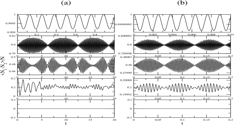
Figure 5: Relative number expectation values for (a) the Josephson regime ($k/{\cal E}_{\mathcal{J}}=1$); (b) between the Josephson and Fock regimes ($k/{\cal E}_{\mathcal{J}}=N$). The initial states are, from top to bottom: $|100,0\rangle,|90,10\rangle,|74,26\rangle,|60,40\rangle$ and $|50,50\rangle$.

As we vary the coupling ratio past the self-trapping threshold value we find an entirely different scenario. In fig. 5 the expectation value for the relative number of particles shows a variety of different behaviours. The dynamics is harmonic when the initial state corresponds to all particles in the same subsystem, and the oscillation amplitude is small. As the imbalance in the initial state decreases, we first see harmonic modulation of the amplitude of the oscillations, in stark contrast to the cases shown in fig. 4. Note here that the period of the modulation does not depend on the initial state. It is important to mention that in the interval $k/{\cal E}_{\mathcal{J}}\in[1/N,1]$, which is not shown, we find that the crossover from collapse and revival sequences of oscillations with zero mean to oscillations with mean approximately equal to the initial imbalance occurs at $k/{\cal E}_{\mathcal{J}}=4/N$, as expected.

When using other initial states, we can classify them into two categories: symmetric, such as a cat-state

$$|\phi_{\rm CAT}\rangle=\frac{1}{\sqrt{2}}(|N,0\rangle+|0,N\rangle)$$ (4)

and a maximally entangled state

$$|\phi_{\rm ME}\rangle=\frac{1}{\sqrt{N+1}}\sum_{n=0}^{N}|N-n,n\rangle,$$ (5)

or non-symmetric, such as $|N,0\rangle,|N-10,10\rangle,$ etc. The expectation value for the number of particles of any symmetric initial state is zero, due to symmetry of the Hamiltonian under interchange of the two subsystems. In such a case some insight into the behaviour of the system can be gleaned by investigating the variance of the imbalance, which will be explored in the next section.

When a non-zero external potential $\Delta\mu$ is added to the system, some new features appear in the various regimes. In the extreme Rabi regime, the imbalance population oscillates around zero, similar to the $\Delta\mu=0$ case, but here the dependence on the initial state is different and in particular the oscillation amplitude is not zero using the initial state $|N/2,N/2\rangle$. Another important point is that the initial states $|n_{1},n_{2}\rangle$ and $|n_{2},n_{1}\rangle$ produce the same expectation value behaviour. In the crossover between Rabi and Josephson regimes, a different behaviour is found: the oscillation amplitude of the number of particles also depends on the initial state, but here the initial states $|n_{1},n_{2}\rangle$ and $|n_{2},n_{1}\rangle$ do not produce the same expectation value behaviour. The symmetry breaking of the Hamiltonian due to the term $\Delta\mu$ is prominent in this case.

In the Josephson and Fock regimes the introduction of the external potential only produces a significant difference in comparison to the $\Delta\mu=0$ case when the initial imbalance is small. If we consider an initial state where the imbalance population is large, then the two initial states $|m,n\rangle$ and $|n,m\rangle$ produce essentially the same results, while when $|m-n|$ is close to zero the same initial states produce different results. This aspect can be understood when we write down the first two terms of the Hamiltonian (1) in the following way:

$$\left(\sqrt{\frac{k}{8}}(N_{1}-N_{2})-\sqrt{\frac{1}{2k}}\Delta\mu\right)^{2}-\frac{1}{2k}\Delta\mu^{2}.$$

When the fluctuations in the imbalance are small, we see from the terms in the brackets that the external potential will be dominant when

$$\Delta\mu>\frac{k}{2}\langle N_{1}-N_{2}\rangle.$$

This means that the largest effect of the external potential will generally occur when the initial state is symmetric.

4 Imbalance fluctuation and entanglement

Here we will study the extent to which the evolution of the imbalance variance and the entanglement are correlated, and how the choice of initial state, as well as the coupling regime, determine the main features of the evolution. On one hand, any state of the system (with fixed $N$) which is unentangled must have zero fluctuation in the imbalance. The converse however is not true, as the cat-state (4) has maximal imbalance variance but relatively small entanglement, and the maximally entangled state (5) has smaller imbalance variance than (4).

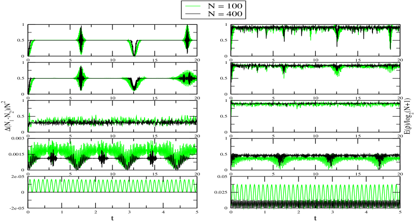
Figure 6: Time evolution of the relative particle number fluctuations (on the left) and entanglement (on the right) for the initial state $|N,0\rangle$ where $N=100,\,400$. From top to bottom the ratio of couplings used are $k/{\cal E}_{\mathcal{J}}=1/N^{2},1/N,4/N,10/N,1$.

For the results shown in fig. 6, we have chosen $|N,0\rangle$ as the initial state, which is unentangled. In the coupling regime $k/{\cal E}_{\mathcal{J}}\in[1/N^{2},1/N]$ where the tunneling is strong, we find that the behaviour of the variance of the relative particle number is similar to the collapse and revival character of the expectation value (cf. fig. 1). We can observe that the entanglement quickly approaches the maximum value and for all later times the system is mostly entangled. At the threshold coupling $k/{\cal E}_{\mathcal{J}}=4/N$, there is no collapse and revival behaviour in the imbalance variance and we see that the mean value starts to decrease. Beyond the threshold coupling, the mean value of both the imbalance variance and the entanglement decrease. When the ratio $k/{\cal E}_{\mathcal{J}}=1$ is reached, we find small oscillations close to zero for both the imbalance variance and the entanglement. From here to the Fock regime (not shown), the imbalance variance practically goes to zero and the entanglement essentially disappears.

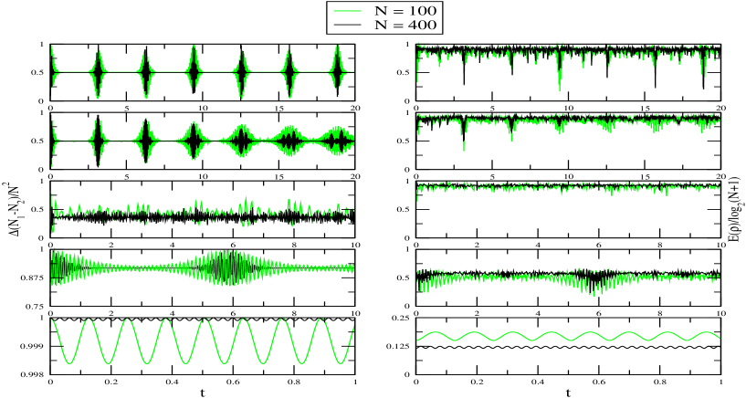
Figure 7: Time evolution of the relative particle number fluctuations (on the left) and entanglement (on the right) for the initial state $|\phi_{\rm CAT}\rangle$ where $N=100,\,400$. From top to bottom the ratio of couplings used are $k/{\cal E}_{\mathcal{J}}=1/N^{2},1/N,4/N,10/N,1$.

For fig. 7, the initial state is the cat-state (4) which has entanglement $E(\rho)=1$. In contrast to fig. 6, the mean value of the imbalance variance increases beyond the threshold coupling. As the ratio $k/{\cal E}_{\mathcal{J}}$ approaches unity, small amplitude periodic oscillations are observed very near to the maximal value of $N^{2}$. For the entanglement the picture is similar to fig. 6. For $k/{\cal E}_{\mathcal{J}}=1$ the entanglement is found to display periodic oscillations about a mean value close to the value for the entanglement of the initial state, which is non-zero in this instance.

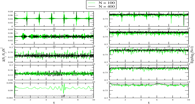
Figure 8: Time evolution of the relative particle number fluctuations (on the left) and entanglement (on the right) for the initial state $|\phi_{\rm ME}\rangle$ where $N=100,\,400$. From top to bottom the ratio of couplings used are $k/{\cal E}_{\mathcal{J}}=1/N^{2},1/N,4/N,10/N,1$.

Finally, fig. 8 shows the results obtained when the initial state is the maximally entangled state (5). Here, a much different behaviour is found in comparison to the previous examples. In the interval $k/{\cal E}_{\mathcal{J}}\in[1/N^{2},1/N]$ the mean values for the variance of the imbalance are smaller than in the previous two examples. At the threshold coupling the mean is substantially larger than the mean value below threshold coupling, and the mean value again decreases as $k/{\cal E}_{\mathcal{J}}$ approaches unity. The most striking feature at $k/{\cal E}_{\mathcal{J}}=1$ is that there is no discernable periodicity in the imbalance variance, whereas in the analogous cases shown in figs. 6, 7 there is clear periodicity. For the entanglement, it appears that the evolution is not substantially dependent on the coupling regime when the initial state is maximally entangled. All cases shown have much the same mean entanglement over time. Like the imbalance variance, there is also no periodicity in the entanglement evolution for the coupling $k/{\cal E}_{\mathcal{J}}=1$.

5 Conclusion

To summarise, we have investigated the quantum dynamics of a model for two Josephson-coupled Bose–Einstein condensates across a wide range of coupling regimes and various initial states, using the method of direct numerical diagonalisation. Our analysis shows that despite the apparent simplicity of the Hamiltonian, diverse features including collapse and revival of oscillations, amplitude modulated oscillations and non-harmonic behaviour are displayed. The most striking changes in the dynamics occur as the system crosses the threshold coupling $k/{\cal E}_{\mathcal{J}}=4/N$.

Acknowledgements

APT thanks CNPq-Conselho Nacional de Desenvolvimento Científico e Tecnológico (a funding agency of the Brazilian Government) for financial support and the Centre for Mathematical Physics at The University of Queensland for kind of hospitality. JL gratefully acknowledges funding from the Australian Research Council and The University of Queensland through a Foundation Research Excellence Award. AF thanks CNPq-Brazil.

References

- [1] S. N. Bose, Z. Phys. 26 (1924) 178
- [2] A. Einstein, Phys. Math. K1 22 (1924) 261
- [3] E. A. Cornell and C. E. Wieman, Rev. Mod. Phys. 74 (2002) 875
- [4] J. R. Anglin and W. Ketterle, Nature 416 (2002) 211
- [5] M. R. Andrews, C. G. Townsend, H. -J. Miesner, D. S. Durfee, D. M. Kurn and W. Ketterle, Science 275 (1997) 637
- [6] E. A. Donley, N. R. Claussen, S. T. Thompson and C. E. Wieman, Nature 417 (2003) 529
- [7] L. You, Phys. Rev. Lett. 90 (2003) 030402
- [8] M. A. Nielsen and I. L. Chuang, Quantum Computation and Quantum Information (Cambridge University Press, Cambridge, 2000)
- [9] J. Willians, R. Walser, J. Cooper, E. A. Cornell, M. Holland, Phys. Rev. A 61 (2000) 033612
- [10] M. R. Mathews, B. P. Anderson, P. C. Haljan, D. S. Hall, M. J. Holland, J. E. Willians, C. E. Wieman and E. A. Cornell, Phys. Rev. Lett. 83 (1999) 3358.
- [11] M. Greiner, O. Mandel, T. Esslinger, T.W. Hänsch and I. Bloch, Nature 415 (2002) 39
- [12] A. J. Leggett, Rev. Mod. Phys. 73 (2001) 307
- [13] G. J. Milburn, J. Corney, E. M. Wright and D. F. Walls, Phys. Rev. A 55 (1997) 4318
- [14] A. P. Hines, R. H. McKenzie and G. J. Milburn, Phys. Rev. A 67 (2003) 013609
- [15] J. R. Anglin, P. Drummond, A. Smerzi, Phys. Rev. A 64 (2001) 063605
- [16] J. Links and H.-Q. Zhou, Lett. Math. Phys. 60 (2002) 275
- [17] H.-Q. Zhou, J. Links, R. H. McKenzie and X. -W. Guan, J. Phys. A: Math. Gen. 36 (2003) L113
- [18] A. Micheli, D. Jaksch, J. I. Cirac and P. Zoller, Phys. Rev. A 67 (2003) 013607
- [19] T. J. Osbourne and M. A. Nielsen, Phys. Rev. A 66 (2002) 032110
- [20] A. Osterloh, L. Amico, G. Falci and R. Fazio, Nature 416 (2002) 608
- [21] M. A. Martín-Delgado, preprint quant-ph/0207026
- [22] L. Sanz, R. M. Angela and K. Furaya, J. Phys. A: Math. Gen. 36 (2003) 9737
- [23] Y. Makhlin, G. Schön and A. Shnirman, Rev. Mod. Phys. 73 (2001) 357
- [24] C. H. Bennett, H. J. Bernstein, S. Popescu and B. Schumacher, Phys. Rev. A 53 (1996) 2046