Separability Analyses of Two-Qubit Density Matrices

Abstract

We pursue a number of analytical directions, motivated to some extent initially by the possibility of developing a methodology for formally proving or disproving a certain conjecture of quantum-theoretical relevance (quant-ph/0308037). It asserts that the 15-dimensional volume occupied by the separable two-qubit density matrices is $(\sqrt{2}-1)/3$, as measured in terms of the statistical distinguishability metric (four times the Bures or minimal monotone metric). Somewhat disappointingly, however, the several various analyses that we report, though we hope of independent/autonomous interest, appear to provide small indication of how to definitively resolve the conjecture. Among our studies here are ones of: (1) the Bures volumes of the two-dimensional sections of Bloch vectors for a number of the Jakóbczyk-Siennicki two-qubit scenarios; (2) the structure of certain convex polytopes of separable density matrices; and (3) the diagonalization of $15\times 15$ Bures metric tensors.

I Introduction

In a previous study Slater (a), we formulated — based on some combination of numerical and analytic evidence — a conjecture that the volume, as measured in terms of the statistical distinguishability (SD) metric Braunstein and Caves (1994), of the 15-dimensional convex set of $4\times 4$ separable density matrices is

$$V_{SD}^{sep}=(\sqrt{2}-1)/3\approx 0.138071.$$ (1)

The numerator of (1), that is $\sigma_{Ag}\equiv\sqrt{2}-1$ (alternatively, $\sqrt{2}+1=1/(\sqrt{2}-1)$), has been previously termed the “silver mean” Christos and Gherghetta (1991). It is interesting to note that this SD conjecture (1) involves the first three positive integers alone, while the “golden mean” Livio (2002) is defined as $(\sqrt{5}+1)/2$ (or, alternatively as $(\sqrt{5}-1)/2=2/(\sqrt{5}+1)$).

A numerical integration based on two billion (separable and nonseparable) density matrices generated by a quasi-Monte Carlo (Faure-Tezuka) procedure had yielded an estimate of 0.137884 for $V^{sep}_{SD}$ Slater (a). (It now appears Slater (b) that it is possible to significantly accelerate the MATHEMATICA program employed, so that we may soon be able to report results for substantially larger sample sizes.) In Slater (2000a), an exact Bures probability of separability ($V^{sep}_{Bures}/V^{sep+nonsep}_{Bures}$) equal to $\sigma_{Ag}$ had been obtained for both the $q=1$ and $q=\frac{1}{2}$ two-qubit states Abe and Rajagopal (1999) inferred using the principle of maximum nonadditive [Tsallis] entropy — and also for an additional low-dimensional scenario (Slater, 2000a, sec. 2.2.1).

Since the Bures (minimal monotone Petz and Sudár (1996)) metric Hübner (1992, 179) is identically one-fourth the SD metric Braunstein and Caves (1994), that is

$$d_{Bures}(\rho,\rho+d\rho)^{2}=(1/4)d_{SD}(\rho,\rho+d\rho)^{2},$$ (2)

in the neighborhood of a density matrix $\rho$, the conjecture (1) becomes equivalent to one that the Bures volume is

$$V_{Bures}^{sep}=2^{-15}(\sqrt{2}-1)/3\approx 4.2136\cdot 10^{-6}.$$ (3)

(In Slater (a), we had also been led to a number of related conjectures, including one that $V^{sep}_{KM}=30V^{sep}_{Bures}$, for the two-qubit systems, where $KM$ denotes the Kubo-Mori monotone metric.)

In the present analysis, we undertake a line of research that hopefully — we, at least, initially thought — may contribute to formally proving/disproving this conjecture. This has seemed a quite formidable task, as a (naive “brute force”) symbolic integration approach, along the lines of the high-dimensional numerical integration followed in Slater (a), appears to be far beyond present computing technology (cf. Slater (b)). In this previous work Slater (a), we generated $4\times 4$ density matrices, which then had to be checked for possible separability. Here, our approach focuses at the outset on separable density matrices, and the nonseparable ones do not directly enter the picture (cf. Aravind (1997); Ericsson (2002); Kuś and Życzkowski (2001)).

The convex domain ($D$) of $4\times 4$ separable density matrices is 15-dimensional in nature. In sec. II.1 we systematically generate 16 pure product $4\times 4$ separable density matrices, convex combinations of these sixteen spanning some subset of $D$. (The entire domain $D$ itself, however, is the closed convex hull of the set of all — not just 16 — product states Clifton and Halverson (2000).) This approach can be interestingly contrasted (in sec. II.4) with that of Braunstein et al Braunstein et al. (1999), who used — in the $4\times 4$ case — an overcomplete basis of 36 density matrices to “give a constructive proof that all mixed states of $N$ qubits in a sufficiently small neighborhood of the maximally mixed state are separable”. They allowed negative weights on their basis matrices in their analysis, thus enabling them to obtain entangled density matrices. We view the convex weights ($w_{i},i=1,\ldots,15$) attached to the first of our 15 matrices as the parameters or variables of our problem. (Of course, then, we must have $w_{16}=1-\Sigma_{i=1}^{15}w_{i}$ as a bound or dependent parameter.)

Proceeding onward, in sec. II.2 we investigate the possibility of using certain of the results in sec. II.1 to obtain bounds on $V^{sep}_{Bures}$. We examine in sec. II.3 the associated $15\times 15$ Bures metric tensor, and in sec. II.4 consider the use of an overcomplete basis. In sec. II.5, we generate a polytope composed of $8\times 8$ three-qubit density matrices, while we obtain in sec. II.6 the Bures metric tensor in diagonal form. We obtain and plot in sec. II.7 the Bures volume elements for three of the two-dimensional two-qubit scenarios presented by Jakóbczyk and Siennicki Jakóbczyk and Siennicki (2001), and derive the associated “Euclidean” probabilities of separability.

II Analyses

II.1 Convex Polytope of $4\times 4$ Density Matrices

To generate the 16 extreme pure product basis matrices (cf. DiVincenzo et al. (2003); Pittenger (2003)), we start with four $2\times 2$ density matrices, the Bloch vectors of each of which extend to one of the four points $((v,v,v),(-v,-v,v),(-v,v,-v)$ and $(v,-v,-v)$, where $v=1/\sqrt{3}$) of an inscribed tetrahedron (a Platonic solid). Then, we obtain 16 extreme points of $D$, by taking all possible tensor products of pairs of these four $2\times 2$ density matrices. (We note that Schack and Caves (Schack and Caves, 2000, sec. 2.4) mentioned the possibility of this construction, among others, observing that the “4 projectors for a tetrahedron are linearly independent, making the corresponding tetrahedral representation [of a $2\times 2$ density matrix] unique”.)

These 16 extreme pure product density matrices have an interesting structure. Each one is a Bures distance of $\sqrt{2-2/\sqrt{3}}\approx 0.919402$ (and a Hilbert-Schmidt distance Życzkowksi and Sommers (2003) of $2/\sqrt{3}\approx 1.1547$) from six other matrices, and a Bures distance of $2/\sqrt{3}\approx 1.1547$ (and a HS distance of $4/3\approx 1.3333$) from the nine remaining matrices. (Using the trace of the matrix product of pairs of these matrices, as an alternative distance measure, we get the results 1/9 [for six] and 1/3 [for nine].) The Bures distance between two density matrices ($\rho_{1}$ and $\rho_{2}$), given by the formula,

$$d_{Bures}(\rho_{1},\rho_{2})=\sqrt{2-2\mbox{Tr}[(\rho_{1}^{1/2}\rho_{2}\rho_{1}^{1/2})^{1/2}}],$$ (4)

can only yield distances in the range $[0,\sqrt{2}]$. The Hilbert-Schmidt distance is defined as (Życzkowksi and Sommers, 2003, eq. (2.3))

$$d_{HS}(\rho_{1},\rho_{2})=||\rho_{1}-\rho_{2}||_{HS}=\sqrt{\mbox{Tr}[(\rho_{1}-\rho_{2})^{2}]}.$$ (5)

Let us also observe that an explicit distance formula is presently available for just one other “monotone” metric than the Bures, that is, the Wigner-Yanase metric (Gibilisco and Isola, 2003, eq. (5.1)), namely,

$$d_{WY}(\rho_{1},\rho_{2})^{2}=4\mbox{arccos}^{2}{\Big{(}\mbox{Tr}[\rho_{1}^{1/2}\rho_{2}^{1/2}]\Big{)}}.$$ (6)

(The class of all monotone metrics has, of course, a nondenumerable number of members.) In Fig. 1, we show a graph representation — in which only the links corresponding to the Bures distance $\sqrt{2-2/\sqrt{3}}\approx 0.919402$ are allowed — with the 16 extreme density matrices serving as the nodes. (The spectrum Cvetković et al. (1980); Biggs (1993) of the associated (0,1)-adjacency matrix consists of the integers 6, -2 [nine-fold] and 2 [six-fold].)

Figure 1: Graph representation of the 48 links between pairs of the 16 extreme pure product separable density matrices corresponding to a Bures distance equal to $\sqrt{2-2/\sqrt{3}}\approx 0.919402$ (and Hilbert-Schmidt distance of $2/\sqrt{3}\approx 1.1547$). The 16 nodes are grouped into four quartets.

In Fig. 2, we show a graph representation — in which, now, only those edges corresponding to the Bures distance of $2/\sqrt{3}\approx 1.1547$ are displayed. (Its spectrum consists of the integers 9, 1 [nine-fold] and -3 [six-fold].)

Figure 2: Graph representation of the 72 links between pairs of the 16 extreme pure product separable density matrices corresponding to a Bures distance equal to $2/\sqrt{3}\approx 1.1547$ (and Hilbert-Schmidt distance of $4/3\approx 1.33333$.)

II.2 Volume calculations

Additionally, the 16 extreme density matrices (and, it would seem any pure state, in general) are each a Bures distance of 1 (and a HS distance of $\sqrt{3}/2\approx 0.866025$) from the fully mixed state $I_{4}$. (The WY-distance from each of the extreme 16 matrices to $I_{4}$ is $2\pi/3$.) Now, a 15-dimensional Euclidean ball of radius 1 has a volume equal to $256\pi^{7}/2027025\approx 0.381443$ and one of radius $\sqrt{3}/2\approx 0.866025$, a volume equal to $27\sqrt{3}\pi^{7}/3203200\approx 0.044095$. These Euclidean volumes are certainly larger than the Bures and HS volumes of the separable plus nonseparable $4\times 4$ density matrices. These two latter values (precisely known only recently, making use of the theory of random matrices (Sommers and Życzkowski, 2003, eq. (4.12)) (Życzkowksi and Sommers, 2003, eq. (4.5))) are, respectively,

$$V_{Bures}^{sep+nonsep}=\frac{\pi^{8}}{165150720}\approx 0.0000574538;\hskip 14.22636ptV_{HS}^{sep+nonsep}=\frac{\pi^{6}}{851350500}\approx 1.12925\cdot 10^{-6}.$$ (7)

(Also, in Slater (a), we had been led to conjecture that, in the two-qubit case, $V^{sep+nonsep}_{KM}=64V^{sep+nonsep}_{KM}$, where denotes the Kubo-Mori monotone metric.) This Bures volume, remarkably, is the same as the 15-dimensional volume (“hypersurface area”) of a 15-dimensional Euclidean hemisphere (cf. Uhlmann (1996)) with radius 1 Sommers and Życzkowski (2003); Slater (a). (In the numerical integration (Slater, a, sec. 1.2) based on two billion sampled points, a very close estimate of 0.000574536 was obtained for $V^{sep}_{Bures}$.) Coupling this with the “silver mean” conjecture (3) easily yields an implied conjecture that the Bures “probability of separability” Życzkowski et al. (1998) is

$$P^{sep}_{Bures}=\frac{V_{Bures}^{sep}}{V_{Bures}^{sep+nonsep}}=\frac{(1680(\sqrt{2}-1)}{\pi^{8}}\approx 0.0733389.$$ (8)

The scalar curvature of the Bures metric at the fully mixed state $I_{4}$ is known — as a specific case of more general formulas (Dittmann, 1999a, Cor. 3) — to equal 570. We can, thus, attempt to apply the formula (Andai, 2003, p. 3676) (cf. (Petz, 2002, p. 936)),

$$V(B_{r}(\rho_{0}))=\frac{\sqrt{\pi^{n^{2}-1}}r^{n^{2}-1}}{\Gamma{(\frac{n^{2}+1}{2})}}\cdot\Big{(}1-\frac{\zeta(\rho_{0})r^{2}}{6(n^{2}+1)}+O(r^{4})\Big{)},$$ (9)

for the volume of a geodesic ball centered at the $n\times n$ density matrix $\rho_{0}$, where $\zeta(\rho_{0})$ is the scalar curvature at $\rho_{0}$. (The scalar curvature of the [monotone] Wigner-Yanase metric is a constant over the domain of $n\times n$ density matrices equal to $\frac{1}{4}(n^{2}-1)(n^{2}-2)$ (Gibilisco and Isola, , Thm. 7.2), which gives us “only” $52.5$ for $n=4$.) Taking the radius of the ball as $r=1$, and $\zeta(\rho_{0})=570$, $n=4$ and $\rho_{0}=I$, we get the result $V(B_{1}(I_{4}))=512\pi^{7}/883575\approx-1.75015$ plus a higher-order term. (Note the negative sign! So, it appears that more explicit terms in the asymptotic expansion (9) are needed to try to avoid this. In his dissertation, A. Andai has such an expansion (with an $O(r^{8})$ term), but considerably more differential-geometric information is needed beyond the scalar curvature to implement it (cf. Gray and Vanhecke (1979)).

If we fully mix, not the 16 extreme matrices, but only 15 of them in turn (the 15 nonzero $w_{i}$’s all equalling 1/15), we find that the resulting 16 density matrices are all a Bures distance of $\sqrt{2-2\sqrt{3/5}-1/\sqrt{5}}\approx 0.0599422$ (and a HS-distance of $1/(10\sqrt{3})\approx 0.057735$) from $I_{4}$. A 15-dimensional Euclidean ball with this radius has a volume of only
$256(10-\sqrt{5}-2\sqrt{15})^{15/2}\pi^{7}/(158361328125\sqrt{5})\approx 1.76774\cdot 10^{-19}$ (the comparable HS figure being $1.00698\cdot 10^{-19}$). Corresponding application of the formula (9) gives us a quite similar estimate of the Bures volume of $1.73225\cdot 10^{-19}$ (plus a higher-order term) of our 15-dimensional convex body of separable states.

If we fully mix only 14 of the 16 (the 14 nonzero $w_{i}$’s all equalling 1/14), then the resultant Bures distance from $I_{4}$ is either 0.0810507 (for 72 of the possible pairs) or 0.0973228 (for the other 48 possible pairs). (The comparable HS-distances are $\sqrt{11}/42\approx 0.0789673$ and $(\sqrt{5/3})/14\approx 0.0922139$.)

II.3 Bures metric tensor

Using our convex geometry/parameterization, we can further compute (Dittmann, 1999b, Prop. 2) the $15\times 15$ Bures metric tensor ($||g_{ij}||$) at $I_{4}$. (This fully mixed state is obtained by setting $w_{i}=1/16$ for all $i$, in forming the convex combination of the 16 extreme product basis matrices.) It has five eigenvalues equal to $17/s$, where $s=98304=2^{15}\cdot 3$, eight equal to $17/(3s)$ and a pair $17(31\pm\sqrt{769})/(6s)$, having the approximate values 0.00169725 and 0.000094224, being the roots of the quadratic equation

$$(2^{26}\cdot 3^{3})x^{2}-(2^{11}\cdot 3\cdot 7\cdot 31)x+17^{2}=0.$$ (10)

If we transform this tensor by the Jacobian (the determinant of which equals $2^{14}\sqrt{2}$) corresponding to returning from our choice of basis variables to that relying upon the naive parameterization of a two-qubit density matrix, say,

$$\begin{pmatrix}a_{11}&a_{12}+b_{12}i&a_{13}+b_{13}i&a_{14}+b_{14}i\\ a_{12}-b_{12}i&a_{22}&a_{23}+b_{23}i&a_{24}+b_{24}i\\ a_{13}-b_{13}i&a_{23}-b_{23}i&a_{33}&a_{34}+b_{34}i\\ a_{14}-b_{14}i&a_{24}-b_{24}i&a_{34}-b_{34}i&1-a_{11}-a_{22}-a_{33},\end{pmatrix}$$ (11)

we can obtain the invariant trace of the Bures metric tensor (cf. Frieden (1998)), which is $255/2^{16}$. The square root of the determinant of the transformed tensor gives us the invariant volume element at $I_{4}$. This we computed to equal $2^{-120}17^{7}\sqrt{17/2}\approx 9.00021\cdot 10^{-28}$.

If we allow the weight ($w_{1}$) assigned to the first, say, of the 16 matrices to vary between 0 and 1/8, and the weight ($w_{16}=1/8-w_{1}$) compensatingly likewise, keeping the fourteen other weights as 1/16, the determinant of the $15\times 15$ Bures metric tensor is a (high) 80-degree polynomial in $w_{1}$, but the graph (Fig. 3) of its square root multiplied by the Jacobian determinant (that is, the corresponding volume element $|g_{ij}|^{1/2}$) seems quite well-behaved — clearly peaking at $w_{1}=w_{16}=1/16$, that is at $I_{4}$. The integral of this function over [0,1/8] is $9.38545\cdot 10^{-29}$ — a result certainly not inconsistent with our “silver mean” conjecture (3) for the total Bures volume $V_{Bures}^{sep}$ of $D$, the full 15-dimensional convex set of $4\times 4$ separable states. The Bures distance between the two extremes on this plot (that is, one state with $w_{1}=0,w_{16}=1/8$ and one with $w_{1}=1/8,w_{16}=0$, while all other $w$’s remain fixed at 1/16) is $(6-\sqrt{34})/6\approx 0.0281747$, considerably larger than the indicated integral between these two endpoints.

Figure 3: Plot of volume element of $15\times 15$ Bures metric tensor in the neighborhood of the fully mixed state $I_{4}$, as a function of $w_{1}$ over the range [0,1/8], with $w_{i}=1/16$ for $i=2,\ldots,15$ and $w_{16}=1/8-w_{1}$. For $w_{1}=w_{16}=1/16$, one gets $I_{4}$. The function peaks at $I_{4}$, having the exact value $2^{-120}17^{7}\sqrt{17/2}\approx 9.00021\cdot 10^{-28}$ there.

In Fig. 4 we show the same form of plot as Fig. 3, but now using the trace of the $15\times 15$ metric tensor rather than the volume element.

Figure 4: Plot of trace of $15\times 15$ Bures metric tensor in the neighborhood of the fully mixed state $I_{4}$, as a function of $w_{1}$ over the range [0,1/8], with $w_{i}=1/16$ for $i=2,\ldots,15$ and $w_{16}=1/8-w_{1}$. For $w_{1}=w_{16}=1/16$, one gets $I_{4}$. The function peaks at $w_{1}=1/16$ with the value $255/2^{16}\approx 0.00389099$ there.

We were not able to compute determinants of the $15\times 15$ metric tensor when more than one of the convex weights was allowed to freely vary. (We were also unable to express a Bell state as a linear combination — of course, requiring negative weights — of the 16 extreme pure product density matrices.)

II.4 Overcomplete Basis

If we were to use in the two-qubit case, not the 16 extreme density matrices employed above, but the 36 extreme density matrices (forming an overcomplete basis), applied by Braunstein et al Braunstein et al. (1999), then we find that of the $35\cdot 36/2=630$ possible distinct unordered pairs of density matrices, 144 correspond to a Bures distance of $\sqrt{2-\sqrt{2}}$, 198 to $\sqrt{2}$ and 288 to 1. (Thus, as opposed to the analysis based on the 16 matrices, there are three, not two different sets of internodal distances.) In Fig. 5, we represent those 144 links with a Bures distance of $\sqrt{2-\sqrt{2}}$.

Figure 5: Graph representation of the 144 links between pairs of the 36 extreme pure product separable density matrices — based on the overcomplete “Pauli” basis of Braunstein et al Braunstein et al. (1999) for the two-qubit case — corresponding to a Bures distance equal to $\sqrt{2-\sqrt{2}}$. The nodes are grouped into sextets.

II.5 Convex Polytope of $8\times 8$ Density Matrices

We also extended the general approach above to the three-qubit case, by taking tensor products of all possible triplets of the same four $2\times 2$ density matrices with their Bloch vectors reaching the points of the inscribed tetrahedron. (The extension to the qubit-qutrit case seems more problematical, since there seems to be no natural immediate analogue of the tetrahedron to employ for choosing nine $3\times 3$ density matrices to tensor product with the four $2\times 2$ density matrices we have been utilizing.) This gives us 64 extreme product triseparable states. There are, then, $63\cdot 64/2=2016$ distinct pairs of intermatrix Bures distances. Of these, 288 are $\sqrt{2-2/\sqrt{3}}\approx 0.919402$, 864 are $2/\sqrt{3}\approx 1.1547$ and another 864 are $\sqrt{2-2/(3\sqrt{3})}\approx 1.27087$. (The corresponding HS-distances are $2/\sqrt{3}\approx 1.1547$, $4/3\approx 1.33333$ and $2\sqrt{13/3}/3\approx 1.38778$.)

In Fig. 6, we show a graph representation — in which only the edges corresponding to the Bures distance $\sqrt{2-2/\sqrt{3}}\approx 0.919402$ are allowed — with the 64 extreme density matrices serving as nodes. (The spectrum of the associated (0,1)-adjacency matrix consists of the integers 9, 5 [nine-fold], -3 [27-fold] and 1 [27-fold]. For the graph based on the Bures distance $2/\sqrt{3}$, the spectrum has 27, -5 [27-fold], and 3 [36-fold] and that based on $\sqrt{2-2/(3\sqrt{3})}$, 27, -9 [nine-fold], 3 [27-fold] and -1 [27-fold].) Graph representations with the other two possible links are perhaps too dense visually for a meaningful representation.

Figure 6: Graph representation of the 288 links between pairs of the 64 extreme pure product triseparable density matrices having Bures distance equal to $\sqrt{2-2/\sqrt{3}}\approx 0.919402$ (and Hilbert-Schmidt distance equal to $2/\sqrt{3}\approx 1.1547$). The 64 nodes fall into 4 groups of 16.

The 64 extreme matrices are all a Bures distance of $\sqrt{2-1/\sqrt{2}}\approx 1.13705$ (and a HS-distance of $\sqrt{7/2}/2\approx 0.935414$) from the fully mixed state $I_{8}$. Euclidean 35-dimensional balls of these radii have volumes of 0.0000299764 and $3.23277\cdot 10^{-8}$, respectively. (The formula (9) — taking into account that the scalar curvature at $I_{8}$ equals 9954 Dittmann (1999a)— gives us a “volume” $1.03199\cdot 10^{-14}$, but with a minus sign.) The trace of the associated $63\times 63$ Bures metric tensor was found at $I_{8}$ to equal $7/2^{74}$. The square root of the determinant of the tensor equals $(2^{2359}3^{72}\sqrt{2})^{-1}$. (Multiplication by the determinant of the Jacobian of the transformation back to the naive parameterization of the $8\times 8$ density matrices (cf. (11)) would give us the volume element at $I_{8}$.) The spectrum of the tensor consists of 26 eigenvalues equal to $1/(2^{75}3^{3})$, 26 equal to $1/(2^{75}3^{2})$ and 8 equal to $(1/(2^{75}3)$ — plus three ($1.90525\cdot 10^{-22},1.3992\cdot 10^{-24}$ and $6.10756\cdot 10^{-24}$) — that are the roots of the cubic equation,

$$(2^{219}\cdot 3^{6})x^{3}-(2^{145}\cdot 3^{3}\cdot 101)x^{2}+(2^{69}\cdot 3\cdot 499)x-1=0.$$ (12)

We have not, however, yet been able to compute the associated eigenvectors.

II.6 Diagonal $15\times 15$ Bures Metric Tensor

We were not only able — using MATHEMATICA — to find the (four distinct) eigenvalues, given above in sec. II.3, using the parameterization based on the 16 extreme pure product density matrices, of the $15\times 15$ Bures metric tensor at $I_{4}$, but also the associated set of orthonormal eigenvectors. Using the components of these eigenvectors as weights, we performed a linear transformation from the variables $w_{i}$ to a new set, call them $v_{i}$, so that the metric tensor was now diagonal (cf. Tod (1992); Cao (1991)). Additionally, at $I_{4}$, only two of the $v_{i}$’s were nonzero — let us denote them $v_{1}$ and $v_{7}$ (as this is how they arise in the analysis) — and these were precisely the ones associated with the paired eigenvalues that are the roots of the quadratic equation (10). So, at $I_{4}$, all $v_{i}$’s are zero, but for two that are the square roots of the roots of the quadratic equation

$$(2^{9}\cdot 769)x^{2}-(2\cdot 3\cdot 5\cdot 769)x-3^{3}=0.$$ (13)

These square roots are $\sqrt{\frac{15}{512}\pm\frac{399}{512\sqrt{769}}}$, having the approximate values of 0.239581 and 0.0345646. (The larger value is associated with the eigenvector for the larger root of (10).) The 15 $4\times 4$ density matrices weighted by the 15 $v_{i}$’s in the new expansion of a $4\times 4$ density matrix were all traceless $4\times 4$ Hermitian matrices. (They were mutually orthogonal, but their self-inner products did not all have the same value, though certainly they could be rescaled so that they do. If we do, in fact, rescale so that all self-inner products equal 2, then we have that $v_{1},v_{7}=\frac{1}{4}\sqrt{3\pm\frac{83}{\sqrt{769}}}$.) There was also a “constant” term (weighted by no parameter $v_{i}$) in this expansion, which was the density matrix of a pure state. We can write this density matrix as $|j\rangle\langle j|$, where

$$|j\rangle=\frac{1}{\sqrt{6(2+\sqrt{3})}}(-\frac{i(5+3\sqrt{3})}{1+\sqrt{3}},(-\frac{1}{2}+\frac{i}{2})(1+\sqrt{3}),(-\frac{1}{2}+\frac{i}{2})(1+\sqrt{3}),1).$$ (14)

Just as we completed the analysis immediately above, we noticed the appearance of a preprint of Kimura and Kossakowski Kimura and Kossakowski (cf. Byrd and Khaneja (2003)) in which the (somewhat similar) density operator expansion

$$\rho=\frac{\mbox{Tr}\rho}{N}I_{N}+\frac{1}{2}\Sigma_{i=1}^{N^{2}-1}(\mbox{Tr}\rho\lambda_{i})\lambda_{i}$$ (15)

is proposed. Here the $\lambda$’s ($i=1,\ldots,N^{2}-1$) are orthogonal generators of $SU(N)$ which satisfy

$$\mbox{(i)}\lambda_{i}^{\dagger}=\lambda_{i},\mbox{(ii)}\mbox{Tr}[\lambda_{i}]=0,(\mbox{iii})\mbox{Tr}[\lambda_{i}\lambda_{j}]=2\delta_{ij}.$$ (16)

We, then, reran our computer programs using this parameterization (employing the standard generators of $SU(4)$). We found that for the fully mixed state $I_{4}$ (where all $\langle\lambda_{i}\rangle=\mbox{Tr}[\rho\lambda_{i}]$ are equal to zero), not only that the $15\times 15$ Bures metric tensor was diagonal, but also that all its diagonal entries (eigenvalues) were equal to a common value, that is, 17/262144, where $262144=2^{18}$. The square root of the determinant of the tensor was, then, equal to $(17/262144)^{15/2}$, which upon multiplication by the determinant $2^{14}\sqrt{2}$ of the Jacobian for the change-of-variables back to the naive parameterization (11) of the $4\times 4$ density matrices, gives us again the invariant volume element $2^{-120}17^{7}\sqrt{17/2}\approx 9.00021\cdot 10^{-28}$.

Also, when we let one parameter vary freely ($\langle\lambda_{1}\rangle$, say) from 0, the Bures metric tensor remained diagonal, unlike the situation in our earlier analysis. However, it appeared that if we were to let all 15 of the parameters vary freely, then the $15\times 15$ Bures metric tensor is not diagonal. (We generated the [very large] symbolic entries of this tensor and then substituted random values of the 15 parameters, in reaching this conclusion.) This has the practical, as well as theoretical significance that one can readily compute the determinant of a symbolic multivariate diagonal $15\times 15$ matrix, but certainly not one with many off-diagonal nonzero entries.

The $15\times 15$ Bures metric tensor obtained using the naive parametrization (11) is itself quasi-diagonal, with the only off-diagonal structure being the $3\times 3$ submatrix pertaining to the diagonal entries $a_{11},a_{22},a_{33}$. The six off-diagonal nonzero entries are $2^{-17}$ and the 15 diagonal entries are $2^{-16}$. The volume element (square root of the determinant) at $I_{4}$ is, as mentioned previously, $2^{-120}17^{7}\sqrt{17/2}$.

II.7 Jakóbczyk-Siennicki Two-Qubit Analyses

Jakóbczyk and Siennicki Jakóbczyk and Siennicki (2001) studied — using the same $SU(4)$ parameterization (15) as employed by Kimura and Kossakowski Kimura and Kossakowski (which we used to obtain a diagonal equal-entry $15\times 15$ Bures metric tensor [sec. II.6]) — two-dimensional sections of a set of Bloch vectors corresponding to two-qubit density matrices. In an interesting set of diagrams, they depicted both the domains of these $4\times 4$ density matrices (Jakóbczyk and Siennicki, 2001, Fig. 1) and their convex subsets of separable states (Jakóbczyk and Siennicki, 2001, Fig. 2) (in those specific cases in which there were nontrivial inclusions).

We have, first, analyzed the case they denote by the letter C, in which only the sixth and fifteenth $SU(4)$ generators are assigned nonzero weight in the density matrix expansion (15). We found that the total Bures volume (of the indicated triangular domain) was $3.27995\cdot 10^{-6}$. Then, using further results of theirs, we computed the Bures volume of the separable subset to be $6.43885\cdot 10^{-7}$. Thus, the probability of separability (the ratio of these two quantities) Życzkowski et al. (1998); Slater (2000b) for this particular scenario (labeled CK’) was 0.196309. (Viewing the corresponding illustration of the separable and nonseparable regions in (Jakóbczyk and Siennicki, 2001, Fig. 2) simply naively as a Euclidean diagram, we obtain a “Euclidean probability of separability” that is much higher, being the ratio of $1/\sqrt{6}+\sqrt{2}\pi/9$ to $2^{5/2}/3^{3/2}$, that is, $(9+2\pi\sqrt{3})/24\approx 0.82845$. Also, we were not able to compute enough digits of accuracy to meaningfully address the question of whether these quantities might possibly correspond to analytically exact expressions.) In Fig. 7 we show the Bures volume element over this two-dimensional triangular domain of $4\times 4$ density matrices. (The fully mixed state $I_{4}$ corresponds to the origin.)

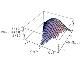
Figure 7: Bures volume element over the triangular domain of two-parameter $4\times 4$ (separable and nonseparable) density matrices, denoted C by Jakóbczyk and Sennini (Jakóbczyk and Siennicki, 2001, Fig. 1). The Bures volume was computed to be $6.43885\cdot 10^{-7}$. The fully mixed state $I_{4}$ is at the origin.

In Fig. 8 we analogously show the Bures volume element for the two-dimensional scenario Jakóbczyk and Siennicki denote by the letter G (in which only the sixth and eighth $SU(4)$ generators are allowed to bear nonzero weight).

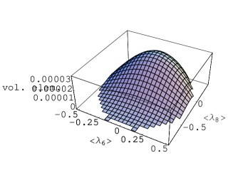
Figure 8: Bures volume element over the elliptical domain of two-parameter $4\times 4$ (separable and nonseparable) density matrices, denoted G by Jakóbczyk and Sennini (Jakóbczyk and Siennicki, 2001, Fig. 1).

As a Euclidean figure, the area of this elliptical domain is $(9\pi\sqrt{3/2})/32\approx 1.08215$, while the area of the separable subdomain is $(9(2+\pi)\sqrt{3/2})/64\approx 0.885535$. The naive Euclidean probability of separability is, then, simply $(2+\pi)/(2\pi)\approx 0.81831$. Our attempts to compute with reasonable confidence the corresponding Bures volumes (and, thus, the Bures probability of separability) were impeded by considerable MATHEMATICA numerical integration difficulties we have not yet resolved.

In Fig. 9 we further show the Bures volume element for the two-dimensional scenario Jakóbczyk and Siennicki denote by the letter E (in which only the third and nineth $SU(4)$ generators are allowed to bear nonzero weight).

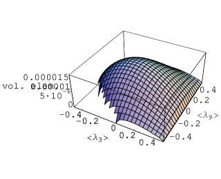
Figure 9: Bures volume element over the hyperbolic domain of two-parameter $4\times 4$ (separable and nonseparable) density matrices, denoted E by Jakóbczyk and Sennini (Jakóbczyk and Siennicki, 2001, Fig. 1).

As a Euclidean figure, the area of this hyperbolic domain is $2\sqrt{2}/3\approx 0.942809$, while the area of the separable subdomain is simply $2/3\approx 0.666667$. The naive Euclidean probability of separability is, then, $1/\sqrt{2}\approx 0.707107$. Our attempts to compute with reasonable confidence the corresponding Bures volumes (and, thus, the Bures probability of separability) were again impeded by numerical integration problems.

III Concluding Remarks

Let us point out a number of papers Kellerhals (1989, 1995); Ratcliffe et al. (1999) (see also (McMullen and Schulte, 2002, Chap. 6)), in which the volumes of non-Euclidean regular polytopes — such as we have encountered in this study (secs. II.1 II.5) — are computed. For an (Euler angle) parameterization of the $4\times 4$ density matrices different from those discussed above, see Tilma et al. (2002). (This parameterization was used in the numerical integration Slater (a), in which the “silver mean” conjectures ((1), (3)) were formulated, as the domain of possible values of the parameters is readily expressible as a 15-dimensional hyperrectangle.)

Let us conclude on something of a discouraging note, however, in so far as we had been hoping initially to be able to report some progress or conceptual breakthrough in formally resolving our “silver mean conjectures” ((1), (3)), as to the statistical distinguishability/Bures volumes of the 15-dimensional convex set of separable two-qubit states. (We continue to pursue the possibility of developing companion conjectures for the 35-dimensional convex set of qubit-qutrit states Slater (b), in terms of the Bures and a number of other monotone metrics, as well as the Riemannian, but non-monotone Hilbert-Schmidt metric Życzkowksi and Sommers (2003); Ozawa (2000).) The analyses presented above — though perhaps of interest from a number of perspectives — appear to help little in this regard.

One possible further approach we have not yet investigated in any depth is the application of the concept of minimal volume Bavard and Pansu (1986); Bowditch (1993); Bambah et al. (1986), seeing that the Bures metric does, in fact, serve as the minimal monotone metric Petz and Sudár (1996). (For a smooth manifold $M$, the minimal volume of $M$ is defined to be the greatest lower bound of the total volumes of $M$ with respect to complete Riemannian metrics, the sectional curvatures of which are bounded above in absolute value by 1 Gromov (1982). We note that lower bounds on the scalar curvature are available from the work of Dittmann Dittmann (1999a).) In Bavard and Pansu (1986), demonstrating a conjecture of Gromov, the minimal volume of $\bf{R}^{2}$ (the infinite Euclidean plane) was shown to be $\frac{2\pi}{\sigma_{Ag}}$. (An exposition of this result is given in Bowditch (1993).) In Bambah et al. (1986) the value of $\frac{1}{2\sigma_{Ag}}$ was obtained for a certain supremum of volumes.