A modulated mirror for atomic interferometry

Abstract

A novel atomic beam splitter, using reflection of atoms off an evanescent light wave, is investigated theoretically. The intensity or frequency of the light is modulated in order to create sidebands on the reflected de Broglie wave. The weights and phases of the various sidevands are calculated using three different approaches: the Born approximation, a semiclassical path integral approach, and a numerical solution of the time-dependent Schr dinger equation. We show how this modulated mirror could be used to build practical atomic interferometers.

1 Introduction.

A number of experimental techniques have been developed to enable the interference of atoms to be observed, as the present special issue illustrates. The essential requirement for producing quantum interference is that a system can pass between two points in its configuration space $\sl via\rm$ more than one path — that is, the quantum amplitude for a passage $\sl via\rm$ either path is non-negligible for a given evolution of the system. The two paths can be visualized as forming a closed loop in configuration-space. If the relative phase between the two quantum amplitudes can vary, then the system can finish in one of two (or more) final states, with probabilities depending on this phase.

The well-known features just mentioned are illustrated by the three main elements of a typical particle interferometer: a first beam splitter, one or more mirrors to bring the two paths back together in position, and a second beam splitter to close the loop. Diffraction or refraction can also be used to play the role of a “mirror” in bending an otherwise straight path for the interfering particle.

In this paper we describe a new beam splitter for neutral atoms, and also show how a practical interferometer can be made, having a number of promising properties such as simplicity, and fairly high (about 8%) transmission efficiency into the useful output states. The beam splitter is a vibrating mirror — that is a surface which reflects atom incident upon it, and which moves rapidly to and fro along the normal direction. Such a beam splitter can form the basis of a number of interferometer designs. An especially interesting possibility is a very simple interferometer having only a $\sl single\rm$ “optical element” — a horizontal mirror is used, and atoms bounce repeatedly on it. Gravity plays the essential role of bringing the atomic trajectories back to the mirror surface, and the same vibrating mirror is used to separate and recombine the interferometer arms.

The ability to create a variety of motions of the mirror surface enables one to manipulate the reflected de Broglie waves in a general manner — both delicate adjustments and large shifts of the atomic momentum can be produced. In the general case, one notes that at normal incidence, the path length for a wave to travel along the $z$-axis from a position $z$, be reflected at $z_{\rm m}$ , and then return to $z$, is $2(z-z_{\rm m})$. By varying $z_{\rm m}$ in time, the variation in path length can be understood as forming an “optical element” such as a prism, lens, or phase grating. Here the “lens” (or other element) is extended in $\sl time\rm$ and affects the motion along the mirror normal $z$, while a conventional lens is extended in $\sl position\rm$ and affects the motion transverse to its axis. Narrow slits and amplitude gratings can be made by switching the mirror reflectivity between one and zero. Our proposal relies on the possibility of vibrating the mirror rapidly (typical vibration frequencies are in the MHz region). This would be difficult for a traditional mirror made of matter, but is easy to achieve for a mirror formed by a light field, since laser beam intensities or frequencies can be modulated rapidly using acousto-optic modulators.

In the following, we first briefly consider beam splitter in general, and the basic principle of the vibrating mirror (Sect. 2). An ideal mirror for atoms would consist of a sharp potential barrier [1]. In practice, one cannot find an ideal mirror, and an important type of mirror for atoms is a quasi-resonant evanescent light wave at the surface of a dielectric [2]. This produces a potential $V\exp(-2\kappa z)$ having an exponential dependence on atomic position $z$. We consider atoms bouncing on such a potential, and calculate the effect of a time-modulation of the amplitude $V(t)$ — for the exponential function, such a modulation is equivalent to moving the potential along the $z$-axis by $z_{\rm m}$ given by

$$V(t){\rm e}^{-2\kappa z}\equiv V(0){\rm e}^{-2\kappa(z-z_{\rm m}(t))}\qquad\mbox{or}\qquad 2\kappa z_{\rm m}(t)=\ln(V(t)/V(0)).$$ (1.1)

In sections 3 and 4 we consider two perturbative methods to calculate the probability for an atom to be scattered by the vibrating mirror from one energy eigenstate (or plane wave) to another. The first method uses the Born approximation in first order; this approximation is valid when the first order scattering probability is low. The second method calculates the phase accumulated by an atom undergoing reflection from a vibrating mirror, using an action integral along the classical path of an atom reflected by a stationary mirror. The range of validity now includes the physically interesting situation where the scattering probability from one eigenstate to another is of the order of 1. In section 5 we consider the case of an initial wave-packet rather than a single plane wave, and compare the approximate analytic results with those of a numerical solution of the Schrödinger equation. This enables us to confirm the validity of the various methods. In section 6 we then go on to consider the application of these ideas to make a realistic atom interferometer.

2 Atom beam splitters.

Up to now many atomic beam splitters have been suggested, and several demonstrated. In the following list we mention the beam splitter used in existing interferometers. These are, to our knowledge, the longitudinal Stark method [3]; the simple Young’s slits arrangement [4, 5]; micro-fabricated gratings [6]; the Raman pulse technique [7, 8]; the optical Ramsey interferometer [9, 10]; and the longitudinal Stern-Gerlach interferometer [11]. There has been rapid progress and some very promising results, in term of the minimum detectable phase shift in a given integration time, combined with a large effective area of the interferometer — both are important since for most experiments the phase change produced by the effects to be measured is proportional to the area of the loop in parameter-space.

Methods to produce larger beam separations have been investigated, notably adiabatic passage in a “dark” state [12, 13]; the magneto-optical beam splitter [14], and Bragg reflection at crystalline surfaces [15]. The Raman pulse method has also already been used to produce very large splittings by the use of many pulses. The vibrating mirror can produce a beam separation $\Delta p$ of the order of several $\hbar\kappa$ for an incident momentum $p=100\hbar\kappa$, as we will show. This allows a useful effective area for the interferometer without making it too sensitive to misalignments. (The parameter $\kappa$ in Eq. (1.1) is of the order of the wave vector for light in resonance with the atomic transition, so $\hbar\kappa$ is approximately equal to the familiar “recoil” momentum.)

The basic idea of the vibrating mirror is familiar from optics. To calculate the effect of a reflection from a mirror whose position $z_{\rm m}$ varies sinusoidally, $z_{\rm m}(t)=z_{0}\sin\omega t$, we assume the incident and refected waves can be written

$$\phi_{\rm inc}(z,t)=\exp i(-kz-\Omega t)$$ (2.1)

$$\phi_{\rm refl}(z,t)\simeq\exp i(kz-\Omega t-u\sin\omega t+\pi)$$ (2.2)

The reflected wave here is an approximate solution of the wave equation, valid when $u\omega\ll\Omega$. We look for a solution having a node on the mirror surface:

$$\phi_{\rm inc}(z_{\rm m}(t),t)+\phi_{\rm refl}(z_{\rm m}(t),t)=0$$ (2.3)

This implies that

$$u=2kz_{0}$$ (2.4)

The reflected wave has a carrier frequency $\Omega$ plus a frequency modulation imposed by the mirror. It can be decomposed into its component frequencies as follows:

$$\exp i(-\Omega t-u\sin\omega t)=\exp(-i\Omega t)\sum_{n=-\infty}^{\infty}J_{n}(u)\exp(-in\omega t).$$ (2.5)

The weight of a given sideband $\Omega\pm n\omega$ is thus given by $|J_{n}(2kz_{0})|^{2}$.

Our vibrating mirror for matter waves works along the same general principles. An atom ar-riving with the momentum $p_{\rm i}$ has an energy $\hbar\Omega=p_{\rm i}^{2}/2M$. After reflection its final momentum $p_{\rm f}$ is given by

$$\frac{p_{\rm f}^{2}}{2M}=\frac{p_{\rm i}^{2}}{2M}+n\hbar\omega$$ (2.6)

where $n$ is a positive or negative integer. For $\hbar\omega\ll p_{\rm i}^{2}/2M$, the momentum transfer $\Delta p=p_{\rm f}-p_{\rm i}$ is simply given by

$$\Delta p\simeq n\frac{\hbar\omega M}{p_{\rm i}}=nq$$ (2.7)

where the elementary momentum spacing $q$ is equal to

$$q\equiv\frac{\hbar\omega M}{p_{\rm i}}$$ (2.8)

The efficiency of the transfer from $p_{\rm i}$ to $p_{\rm f}$, for the case of a vibrating exponential potential, is the subject of the following sections.

3 Perturbative calculation in the Born approximation.

In this section we present a perturbative calculation of the momentum transfer for atoms reflected off a modulated evanescent potential. Since the problem is invariant under a translation parallel to the mirror surface, we only consider the motion along the $z$-axis, defined normal to the surface.

3.1 The coupling between unperturbed states

The Hamiltonian is split into two parts:

$H=H_{0}+V_{1}$

where $H_{0}$ is the un-modulated part:

$$H_{0}=\frac{p^{2}}{2M}+V_{0}\exp(-2\kappa z)$$ (3.1)

This Hamiltonian is responsible for the standard reflection of atoms off the evanescent wave [2]. $V_{0}$ is the light shift of the ground state of the atom at the prism-vacuum interface located at $z=0$. We consider that the atom adiabatically follows the energy state given by (3.1) without emitting any spontaneous photons. For simplicity, we further do not consider possible atom-surface interactions (van der Waals potential, e.g.), supposing that the atom remains far enough from the surface so that these are negligible compared to the evanescent wave potential in $H$. $V_{1}$ is the modulated part of the atom-laser interaction [16]:

$$V_{1}=\epsilon V_{0}\exp(-2\kappa z)\sin(\omega t)$$ (3.2)

We will treat the case that the modulation amplitude $\epsilon$ is between 0 and 1.

We evaluate the efficiency of the momentum transfer along $Oz$ by calculating perturbatively the coupling between eigenstates of the unperturbed Hamiltonian $H_{0}$ induced by the time dependent part $V_{1}$. The eigenstates of $H_{0}$, characterized by their asympotic momenta $p>0$, are given by [17] ($P\equiv p/\hbar\kappa$ is the scaled momentum):

$$\Psi_{P}^{0}(z)=\sqrt{\frac{2P}{\pi L}\sinh(\pi P)}K_{iP}[w(z)]$$ (3.3)

where $K_{iP}[w(z)]$ is the Bessel $K$-function of imaginary parameter $iP$, and

$$w(z)=\frac{\sqrt{2MV_{0}}}{\hbar\kappa}\exp(-\kappa z)$$ (3.4)

These wavefunctions are the eigenfunctions of the unperturbed Hamiltonian $H_{0}$, normalized in a box between $z=0$ and $z=L\gg\kappa^{-1}$.

According to Fermi’s golden rule, the probability for an atom initially in $\Psi_{\rm i}^{0}(z)$ (corresponding to an incident momentum $p_{\rm i}$) to make a transition to $\Psi_{\rm f}^{0}(z)$ (corresponding to a momentum $p_{\rm f}$) is given by:

$$W_{\rm fi}=\frac{1}{\Phi}\frac{\pi}{2\hbar}|\langle\Psi_{\rm f}^{0}|\epsilon V_{0}\exp(-2\kappa z)|\Psi_{\rm i}^{0}\rangle|^{2}\rho(E_{\rm f}=E_{\rm i}\pm\hbar\omega)$$ (3.5)

where $\rho(E_{\rm f}=E_{\rm i}\pm\hbar\omega)$ is the density of states at the final energy:

$$\rho(E_{\rm f}=E_{\rm i}\pm\hbar\omega)=\frac{dn}{dE}=\frac{ML}{\pi\hbar p_{\rm f}}$$ (3.6)

and $\Phi$ corresponds to the flux of the incident atomic wave:

$$\Phi=\frac{p_{\rm i}}{2ML}$$ (3.7)

The coupling term in (3.5) can be obtained analytically [18], yielding:

$$W_{\rm fi}=\frac{\epsilon^{2}\pi^{2}}{64}\sinh(\pi P_{\rm i})\sinh(\pi P_{\rm f})\left\{\frac{(P_{\rm i}+P_{\rm f})(P_{\rm i}-P_{\rm f})}{\sinh(\frac{\pi}{2}(P_{\rm i}+P_{\rm f}))\sinh(\frac{\pi}{2}(P_{\rm i}-P_{\rm f}))}\right\}^{2}$$ (3.8)

We now discuss this result in the limits of large and small momenta $P_{\rm i}$, $P_{\rm f}$, respectively.

3.2 Semiclassical limit

In the limit $P_{\rm i},P_{\rm f}\gg 1$, we may replace by exponentials the sinh function in (3.8) whose arguments are of the order of $P_{\rm i}$,$P_{\rm f}$. The transition probability is then approximated by ($\Delta P\equiv P_{\rm f}-P_{\rm i}$):

$$W_{\rm fi}=\frac{1}{4}\epsilon^{2}P_{\rm i}^{2}\left(\frac{\frac{\pi}{2}\Delta P}{\sinh(\frac{\pi}{2}\Delta P)}\right)^{2}=\frac{1}{4}\epsilon^{2}P_{\rm i}^{2}\beta^{2}(\Delta P)$$ (3.9)

The function

$$\beta(x)=\frac{\frac{\pi}{2}x}{\sinh(\frac{\pi}{2}x)}$$ (3.10)

appearing in (3.9) is equal to unity for $x=0$ and decreases exponentially for $|x|\gg 1$. It describes the decrease of the efficiency of the momentum transfer if the potential undergoes too many oscillations during the reflection of the atom. Indeed the interaction time of the atom with the evanescent wave is given by

$$\tau=\frac{M}{\kappa p_{\rm i}}$$ (3.11)

and the momentum transfer can be written

$$\frac{\Delta p}{\hbar\kappa}\approx\omega\tau\equiv Q$$ (3.12)

where $Q\equiv q/\hbar\kappa$. The rapid decrease of the function $\beta(x)$ means that only a few $\hbar\kappa$ of momentum can be transferred efficiently.

In figure 1, we show $W_{\rm fi}$ at $p_{\rm i}=100\>\hbar\kappa$ for the upper and the lower sideband, as a function of $Q$. Note that the results (3.8) and (3.9) predict an asymmetry in the transfer efficiency between the upper and lower sideband $P_{f\pm}=\sqrt{P_{\rm i}^{2}\pm 2P_{\rm i}Q}$. This asymmetry is due to the fact that the monemtum transfer $\Delta P_{\pm}=P_{f\pm}-P_{\rm i}$ is not the same for the two sidebands :

$$|\Delta P_{+}|-|\Delta P_{-}|\approx-\frac{Q^{2}}{P_{\rm i}}$$ (3.13)

Since the transfer efficiency (3.9) depends strongly on the momentum transfer, this difference shows up in the ratio $W_{+}/W_{-}$ between the weights of the sidebands:

$$\frac{W_{+}}{W_{-}}\approx\exp\left(\pi\frac{Q^{2}}{P_{\rm i}}\right)=\exp\left(\pi\frac{\hbar\omega^{2}M^{2}}{p_{\rm i}^{3}\kappa}\right)$$ (3.14)

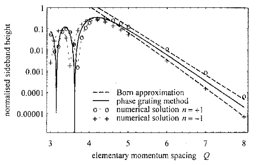
Fig. 1.—: Heights of the sidebands for orders $n=\pm 1$ as a function of $Q\equiv\omega\tau$. The incident momentum is $p_{\rm i}=100\>\hbar\kappa$, and the modulation depth is $\epsilon=1$. The values are normalized to an incident wave with unit amplitude. Dashed lines: the result of the Born approximation, $W_{\rm fi}$ (Eq. (3.8)), multiplied by a factor $p_{\rm i}/p_{\rm f}$ in order to normalize the amplitude of the incident wave. The upper (lower) line corresponds to $n=+1(-1)$. Solid line: result of the semmiclassical approximation, $|a_{1}|^{2}$, (Eq. (4.20)). Circles: numerical solution (Sect. 5) for the normalized momentum distribution $|\psi(p)/\psi(p_{\rm i})|^{2}$ with $p^{2}=p_{\rm i}^{2}+2M\hbar\omega$ (i.e. sideband $n=+1$). For the sake of clarity, the points have been joined in the region $Q<4.2$ (light dashed line). The parameters of the numerical calculation are given in the text (Sect. 5). Crosses: same as before, but now $n=-1$.

3.3 Quantum limit

In the limit of small momenta $P_{\rm i},P_{\rm f}\ll 1$, one expects the evanescent wave mirror to produce the same resuts as a “hard” ideal mirror (Sect. 2.), since the wavelength of the incident atom is then longer than the characteristic decay length $1/2\kappa$ of the mirror potential. In this limit expression (3.8) becomes:

$$W_{\rm fi}\approx\frac{1}{4}\epsilon^{2}P_{\rm i}P_{\rm f}$$ (3.15)

This result can be interpreted by noting that the vibrating evanescent wave mirror, in this regime [17], behaves as an ideal mirror moving as

$$z_{\rm m}(t)=\frac{1}{2\kappa}\ln(1+\epsilon\sin\omega t)$$ (3.16)

For a small modulation amplitude $\epsilon$, this given a sinusoidal variation having amplitude $z_{0}=\epsilon/2\kappa$. Following the discussion of section 2, the weight of the first sideband is then given by $|J_{1}(u)|^{2}\approx u^{2}/4$ where the argument $u=\epsilon P_{\rm i}$ (using Eq. (2.4) and $k=p/\hbar$). The flux into the sideband $P_{\rm f}$ is then given by (3.15), per unit flux in the incident state.

4 Semiclassical path integral approach.

In this section, we present a semi-classical perturbation method which allows us to derive the atomic wave function after reflection off the modulated mirror. This method is similar to the one developed for the problem of atomic wave diffraction by a thin phase grating [19]. It leads to a perturbed wave function which is phase-shifted with respect to the wave function obtained for a non-modulated mirror. The phase shift is simply the integral of the modulated potential along the classical unperturbed trajectory of the bouncing atom. In [19], this method was derived using a Feynman path integral approach which allowed for a detailed study of the approximations involved in the derivation. For the sake of simplicity, we present here an alternative derivation based on a modification of the standard WKB treatment so that it can be applied to a time-modulated potential.

4.1 Phase shift of the semiclassical wave function

Consinder the wave function $\Psi^{0}(z)$ which is an eigenstate of $H_{0}$ at the energy $E_{\rm i}$. We look for a perturbed wave function of the following form

$$\Psi(z,t)=\Psi^{0}(z){\rm e}^{-iE_{\rm i}t/\hbar}\exp(iS_{1}(z,t)/\hbar)$$ (4.1)

where $S_{1}(z,t)$ is a small correction introduced by the modulated part of the potential. The time-dependent Schrödinger equation gives:

$$\frac{\partial S_{1}}{\partial t}-\left(\frac{i\hbar}{m\Psi^{0}(z)}\frac{d\Psi^{0}}{dz}\right)\frac{\partial S_{1}}{\partial z}-\frac{i\hbar}{2M}\frac{\partial^{2}S_{1}}{\partial z^{2}}+\frac{1}{2M}\left(\frac{\partial S_{1}}{\partial z}\right)^{2}=-V_{1}(z,t)$$ (4.2)

In the semiclassical limit, where the de Broglie wavelenght of the particle is much smaller than the typical length scale $\kappa^{-1}$ of the potential $V_{0}(z)$, we can approximate $\Psi^{0}(z)$ in the classically allowed region by the well-known WKB result:

$$\Psi_{WKB}^{0\pm}(z)=\frac{1}{\sqrt{k(z)}}\exp\left(\pm i\int^{z}k(z^{\prime})dz^{\prime}\right)$$ (4.3)

where the local wave vector $k(z)$ is given by

$$k(z)=\frac{1}{\hbar}\sqrt{2M(E_{\rm i}-V_{0}(z))}$$ (4.4)

Using now this result for $\Psi^{0}(z)$, we can write

$$-\frac{i\hbar}{M\Psi_{WKB}^{0\pm}(z)}\frac{d\Psi_{WKB}^{0\pm}}{dz}\approx\pm\frac{\hbar k(z)}{M}=v(z)$$ (4.5)

where $v(z)$ is the classical velocity of the particle moving in the unperturbed potential. It can be either negative (before reflection) or positive (after reflection). Note that we have neglected in (4.5) the derivative of the prefactor of (4.3) which would lead to small corrections. The equation of evolution for $S_{1}$ can now be written

$$\frac{\partial S_{1}}{\partial t}+v(z)\frac{\partial S_{1}}{\partial z}=-V_{1}(z,t)+\frac{i\hbar}{2M}\frac{\partial^{2}S_{1}}{\partial z^{2}}-\frac{1}{2M}\left(\frac{\partial S_{1}}{\partial z}\right)^{2}$$ (4.6)

This equation can be solved formally by the method of characteristics: using the characteristic curve $z_{c}(t)$ defined by

$$\frac{d}{dt}z_{c}(t)=v(z_{c}(t))$$ (4.7)

the left hand side of (4.6) can be written

$$\left(\frac{\partial}{\partial t}+v(z)\frac{\partial}{\partial z}\right)S_{1}=\frac{d}{dt}S_{1}(z_{c}(t),t)$$ (4.8)

The characteristic curve $z_{c}(t)$ is the classical trajectory corresponding to a reflection in the unperturbed potential [17]:

$$z_{c}(t)=\frac{1}{2\kappa}\ln\left[\frac{V_{0}}{E_{\rm i}}\cosh^{2}(t-t_{0})/\tau\right]$$ (4.9)

At the “bouncing time” $t=t_{0}$, the atom reaches its classical turning point.

Substituting (4.8) in (4.6), we have the implicit solution

$$S_{1}(z,t) = {}-\int_{-\infty}^{t}dt^{\prime}V_{1}(z^{\prime}=z_{c}(t^{\prime}),t^{\prime})$$ (4.10)

$${}+\frac{1}{2M}\int_{-\infty}^{t}dt^{\prime}\left(i\hbar\frac{\partial^{2}S_{1}}{\partial z^{2}}-\left(\frac{\partial S_{1}}{\partial z}\right)^{2}\right)(z^{\prime}=z_{c}(t^{\prime}),t^{\prime})$$

In the limit $t\rightarrow-\infty$, (4.10) vanishes and (4.1) then reduces to the unperturbed wave function. We are interested here in the case $t-t_{0}\gg\tau$, when the final time $t$ is in the asymptotic region after the reflection.

We now neglect the second term of the right hand side of (4.10). We will investigate the validity of this approximation in detail later on, but we can justify it here in a few words. We are neglecting a second derivative $\partial^{2}S_{1}/\partial z$ and a second order term $(\partial S_{1}/\partial z)^{2}$. The second derivative should have a small contribution in the semiclassical regime of interest here; its effect is mostly to correct the classical motion and to change the prefactor entering in (4.3). The second order term $(\partial S_{1}/\partial z)^{2}$ should be small compared to the first order term entering in (4.2), since we expect $S_{1}$ itself to be a small correction to the unperturbed wave function.

Using the expression (3.2) for $V_{1}(z^{\prime},t^{\prime})$, the integration in (4.10) now yields the phase shift [20]:

$$\frac{S_{1}(z,t)}{\hbar} = -\frac{\epsilon}{\hbar}\frac{p_{\rm i}^{2}}{2M}\int_{-\infty}^{t}\frac{\sin\omega t^{\prime}}{\cosh^{2}(t^{\prime}-t_{0})/\tau}dt^{\prime}$$ (4.11)

$$= -\epsilon P_{\rm i}\beta(\omega\tau)\sin\omega t_{0}$$

Since we have $t-t_{0}\gg\tau$, this result does not explicitly depend on the upper bound $t$, up to small terms of order $\exp[-2(t-t_{0})/\tau]$.

We recover the function $\beta(\omega\tau)=\beta(Q)$ defined in (3.10). The “bouncing time” $t_{0}(z,t)$ of the classical trajectory (4.9) is fixed such that latter ends at time $t$ at the position $z$: $z_{c}(t)=z$. Expanding the trajectory (4.9) for $t-t_{0}\gg\tau$, we find:

$$z=\xi_{\rm eff}+\frac{p_{\rm i}}{M}(t-t_{0})$$ (4.12)

where the “effective mirror” position $\xi_{\rm eff}$ equals [17]

$$\xi_{\rm eff}(p_{\rm i})=\frac{1}{2\kappa}\ln\left[\frac{V_{0}}{4E_{\rm i}}\right]$$ (4.13)

We obtain finally

$$\frac{S_{1}(z,t)}{\hbar}=-u\sin\left(\omega t-\frac{q}{\hbar}(z-\xi_{\rm eff})\right)$$ (4.14)

where the modulation index $u$ is given by:

$$u=\epsilon P_{\rm i}\beta(Q).$$ (4.15)

4.2 The final energy spectrum

The reflected wave function in the asymptotic region $\kappa z\gg 1$ can now be written

$$\Psi_{\rm fin}(z,t)=C\exp\frac{i}{\hbar}(-E_{\rm i}t+p_{\rm i}z+\hbar\eta+S_{1}(z,t))$$ (4.16)

In this expression $C$ is a normalization factor and $\eta=\eta(p_{\rm i})$ is the phase shift of the wave function due to the reflection off the non-modulated evanescent potential. Replacing $S_{1}(z,t)$ by its expression (4.14), and using (2.5) to expand the result in terms of energy sidebands, we have

$$\Psi_{\rm fin}(z,t)=C{\rm e}^{i\eta}\sum_{n=-\infty}^{\infty}a_{n}\exp\frac{i}{\hbar}(-E_{n}t+p_{n}z)$$ (4.17)

where the $n$’th sideband has energy $E_{n}$ and momentum $p_{n}(q\equiv\hbar\omega M/p_{\rm i})$:

$$E_{n}=E_{\rm i}+n\hbar\omega$$ (4.18)

$$p_{n}=p_{\rm i}+nq$$ (4.19)

and its amplitude $a_{n}$ equals:

$$a_{n}=J_{n}(u)\exp(-inq\,\xi_{\rm eff}/\hbar)$$ (4.20)

Note also that, if the phase of the modulated potential at $t=0$ is shifted by $\phi$, then the phases of the sidebands are shifted accordingly:

$$\omega t\rightarrow\omega t-\phi\qquad\Rightarrow\qquad a_{n}\rightarrow a_{n}{\rm e}^{in\phi}$$ (4.21)

As usual in phase modulation problems, there are two limiting regimes for the result (4.17–4.20), depending on the order of magnitude of the modulation index $u$. For a low modulation index, $u\ll 1$, the Bessel functions $J_{n}(u)$ have magnitude $(u/2)^{|n|}$, and the diffracted spectrum consists essentially of the carrier $n=0$ and the two first sidebands $n=\pm 1$. In this regime, we recover the result (3.9) of the Born approximation for the first sideband, evaluated for a semiclassical momentum $p_{\rm i}\gg\hbar\kappa$:

$$|a_{1}|^{2}=|J_{1}(u)|^{2}\simeq\frac{u^{2}}{4}=\frac{1}{4}\epsilon^{2}P_{\rm i}^{2}\beta^{2}(Q)=W_{\rm fi}$$ (4.22)

where we have assumed in addition $Q\ll P_{\rm i}$ so that $Q\simeq\Delta P$. Note, however, that the semiclassical approach does not account for the asymmetry of the sideband weights (3.14); this property is related to the approximations involved (see below).

The semiclassical result (4.17) and (4.20) extends the Born result (3.9) into the region of high modulation index $u\gg 1$, where several lines are present with an appreciable weight. The most intense lines correspond to $n\sim\pm u$, and they lead to a velocity change for the atom $\Delta v_{\rm at,max}\simeq uq/m$. For $\epsilon\ll 1$, where the vibration of $z_{\rm m}(t)$ is harmonic ($2\kappa z_{\rm m}(t)=\epsilon\sin\omega t$), we can relate $\Delta v_{\rm at,max}$ to the “maximal velocity of the vibrating mirror” $v_{\rm mir,max}=\epsilon\omega/2\kappa$:

$$\Delta v_{\rm at,max}=2v_{\rm mir,max}\beta(Q)$$ (4.23)

For a “hard” mirror formed with a potential step, one would expect simply $\Delta v_{\rm at,max}=2v_{\rm mir,max}$. The reduction factor $\beta(Q)$ ($\beta(Q)\ll 1$ for $Q>1$), which appears either in the modulation index $u$ (see (4.15)) or in $\Delta v_{\rm at,max}$ (see (4.23)) is due to the “softness” of the potential. Indeed, the efficiency of the momentum transfer is proportional to the Fourier transform of the potential “seen” by the atom during the reflection (4.11):

$$V_{0}(z_{c}(t))=\frac{E_{\rm i}}{\cosh^{2}(t-t_{0})/\tau},$$ (4.24)

the transform being evaluated at the modulation frequency $\omega$. Since this Fourier transform has a natural cutoff frequency of the order of $\tau^{-1}$, the transfer efficiency decreases for modulation frequencies larger than this limit, i.e. $Q>1$. The same reduction factor $\beta(Q)$ appears in the classical problem of a particle bouncing on a modulated exponential potential. The equation of motion for the particle is:

$$M\frac{d^{2}z}{dt^{2}}=2\kappa V_{0}{\rm e}^{-2\kappa z}(1+\epsilon\sin\omega t)$$ (4.25)

The energy change in the reflection can be written:

$$E_{\rm f}-E_{\rm i}=\int_{-\infty}^{\infty}M\frac{dz}{dt}\frac{d^{2}z}{dt^{2}}dt=-\epsilon V_{0}\omega\int_{-\infty}^{\infty}\cos(\omega t){\rm e}^{-2\kappa z}dt$$ (4.26)

using an integration by parts. We evaluate this last integral along the atomic trajectory in the non-modulated potential, obtaining

$$\frac{E_{\rm f}-E_{\rm i}}{E_{\rm i}}=-2\epsilon Q\beta(Q)\cos\omega t_{0}$$ (4.27)

The maximal atomic velocity change (for $\cos\omega t_{0}=\pm 1$) is then:

$$\frac{\Delta v_{\rm at,max}}{v_{\rm i}}=\epsilon Q\beta(Q)$$ (4.28)

or

$$\Delta v_{\rm at,max}=\epsilon\frac{\omega}{\kappa}\beta(Q)$$ (4.29)

which is identical to (4.23). Note finally that exactly the same dependence on $Q$ appears in the diffraction of atoms by a standing wave at oblique incidence [21, 19].

4.3 Validity of the semiclassical approach

The first validity condition for a semiclassical approach requires

$$P_{\rm i}\gg 1$$ (4.30)

i.e. an incident de Broglie wavelenght much smaller than the decay lenght of the potential.

A second constraint on the validity of (4.17) results from the use of the method of characteristics. Since the expression (4.11) for $S_{1}(z,t)$ has been obtained by integrating over the classical trajectory of the atoms in the absence of the modulated potential, we require that this classical trajectory is only slightly perturbed by the modulation. Otherwise the perturbative expansion underlying (4.11) would not be possible. This condition is fulfilled in two cases. One can first take a very small modulated potential ($\epsilon\ll 1$); the frequency of the modulation can then be chosen freely. The other option is to take an arbitrarily large modulation factor (up to $\epsilon=1$), but to impose a modulation frequency $\omega$ much greater than the characteristic “frequency” of the bouncing process $1/\tau$, where $\tau$ is the reflection time. The modulated potential then induces a fast atomic micromotion, which is superimposed on the slow unperturbed bouncing motion. In the following, we focus on this second option, since it may lead to important transfer of momentum for the atoms. This condition can be written:

$$\omega\tau=Q\gg 1$$ (4.31)

In the previous calculation, an additional approximation is involved, which consists in neglecting in the expression (4.10) for $S_{1}(z,t)$ the contributions of the terms $\partial^{2}S_{1}/\partial z^{2}$ and $(\partial S_{1}/\partial z)^{2}$. Before going further in a quantitative estimation of the corresponding error, we can point out two consequences of this approximation, which appear clearly in the result (4.17). First, (4.17) does not strictly fulfill the dispersion relation for matter waves $E_{n}=p_{n}^{2}/2M$. Equations (4.18) and (4.19) only constitute a linearized version of this dispersion relation for small $nq$, and this induces a small phase error, that should be compensated by the contribution of these two partial derivatives neglected in (4.10). Secondly the momentum distribution deduced from (4.17) is a symmetric comb centered on $p_{\rm i}$, with sidebands whose weight is proportional to $|a_{n}|^{2}=|a_{-n}|^{2}$. However we know from the Born treatment (Sect. 3) that an asymmetry appears in the spectrum, when the parameter $Q^{2}/P_{\rm i}$ becomes of the order of 1 or larger (see (3.13)). We show now how one can recover this validity condition from a detailed analysis of the contributions of the two partial derivatives mentioned above.

We estimate the magnitude of the second term of the right hand side of (4.10), in order to determine the region of parameter space where it can be neglected with respect to the leading term. As an estimation we take $S_{1}(z,t)=0$ before the bouncing time ($t<t_{0}$), and we use for $t>t_{0}$ the asymptotic expression for $S_{1}^{(0)}(z,t)$ given in (4.14) . We obtain in this way, for $t>t_{0}$:

$$\frac{\partial S_{1}}{\partial z}=uq\cos(\omega t_{0})$$ (4.32)

$$\frac{\partial^{2}S_{1}}{\partial z^{2}}=\frac{uq^{2}}{\hbar}\sin(\omega t_{0})$$ (4.33)

We now choose a time $t$ such that $t-t_{0}$ is larger than the reflection time $\tau$ and we evaluate the two contributions that have been neglected in the integral appearing in (4.10):

$$\left|\frac{i}{2M}\int_{-\infty}^{t}\frac{\partial^{2}S_{1}}{\partial z^{\prime 2}}(z^{\prime},t^{\prime})dt^{\prime}\right|\sim u\frac{Q^{2}}{P_{\rm i}}\frac{t-t_{0}}{2\tau}$$ (4.34)

$$\left|\frac{1}{2M\hbar}\int_{-\infty}^{t}\left(\frac{\partial S_{1}}{\partial z^{\prime}}\right)^{2}(z^{\prime},t^{\prime})dt^{\prime}\right|\sim u^{2}\frac{Q^{2}}{P_{\rm i}}\frac{t-t_{0}}{2\tau}$$ (4.35)

The relative magnitude of these two terms depends on the index of modulation. Equation (4.34) is the leading term in the regime of low modulation index ($u\ll 1$), whereas (4.35) is dominant in the high modulation domain ($u\gg 1$).

We note that the magnitude of the two terms (4.34) and (4.35) increases linearly with time, as expected for corrections to the phase of $\Psi_{\rm fin}(z,t)$ whose role is to restore the correct dipersion relation for the de Broglie wave. In practice, we can evaluate these two terms for a time $t$ located well after the classical turning time $t_{0}$. We take for instance:

$$t-t_{0}\simeq 4\tau$$ (4.36)

After the time $t$, the values of the $a_{n}$ coefficients appearing in the final wave function (4.17) do not change anymore, and we can impose “by hand” the correct dispersion relation; in other words, we then replace the wave function (4.17) by

$$\Psi_{\rm fin}^{\prime}(z,t)=C{\rm e}^{i\eta}\sum_{n}a_{n}\exp\frac{i}{\hbar}(-E_{n}t+p_{n}^{\prime}z)$$ (4.37)

with $p_{n}^{\prime}\equiv\sqrt{2ME_{n}}$.

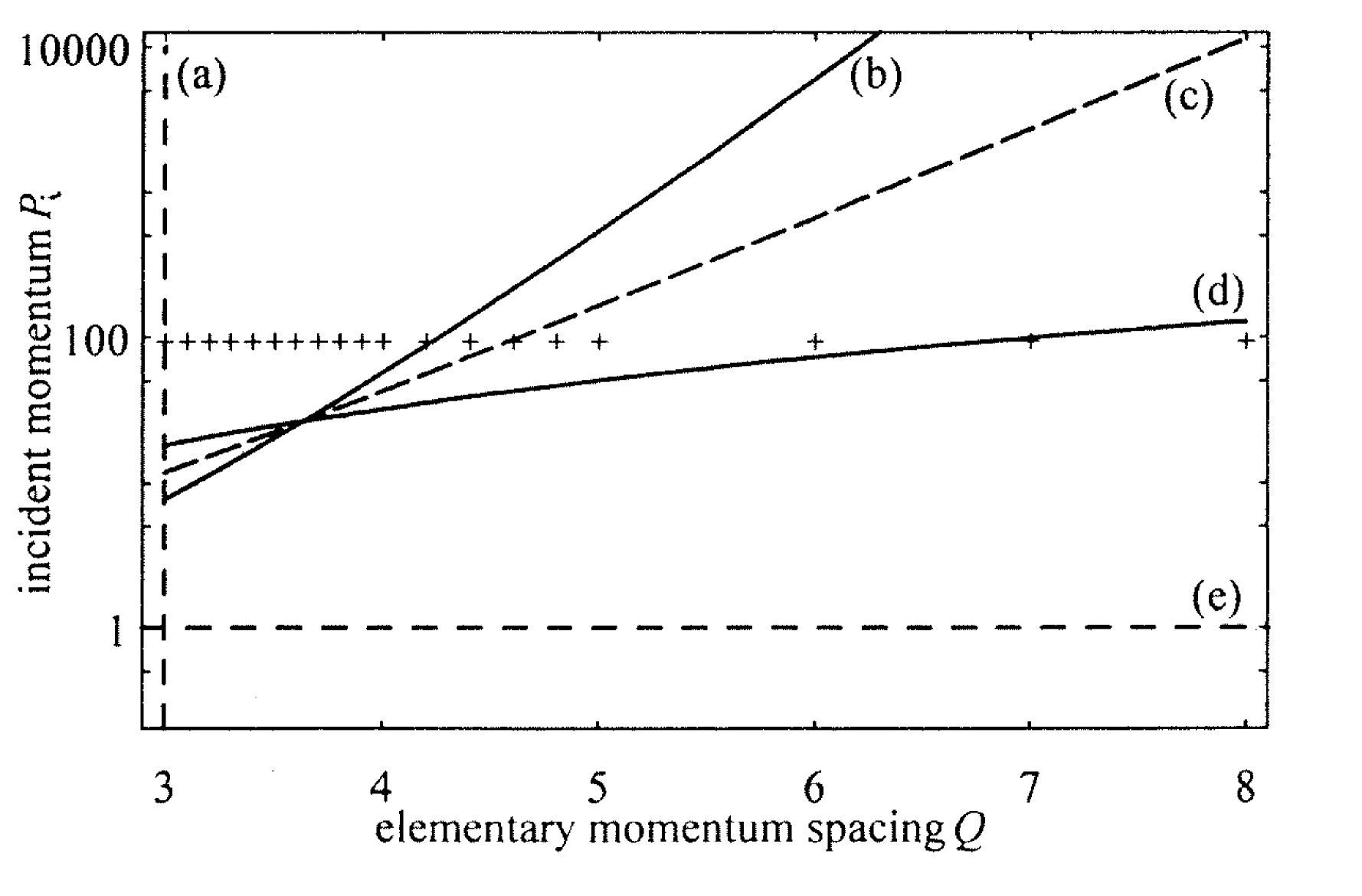
Fig. 2.—: Regions of validity of the semiclassical approach, as a function of $Q$ and $P_{\rm i}=p_{\rm i}/\hbar\kappa$. The modulation depth was taken as $\epsilon=1$. The semiclassical approach is valid in the region between the lines (b) and (d). The line (c) ($u=1$) separates the regimes of high (above) and low (below) modulation index $u$. (a) Line $Q=3$, (Eq. (4.30)) defining the region for a fast classical micromotion of the atom. (b) Limit $2(\Delta P_{max})^{2}=P_{\rm i}$ (Eq. (4.39)). (d) Limit $2Q^{2}=P_{\rm i}$ (Eq. (4.38)). (e) Limiting condition $p_{\rm i}=\hbar\kappa$ for the semiclassical regime. Crosses: parameters corresponding to the numerical solution (Fig. 1 and Sect. 5).

In the regime of low modulation index, the leading correction (4.34) is small compared with the main contribution to $S_{1}/\hbar$ if:

$$2Q^{2}\ll P_{\rm i}$$ (4.38)

As expected, we recover here the condition required for having a quasi-symmetric spectrum.

In the regime of high modulation index, the main contribution to the phase factor $S_{1}/\hbar$ is very large compared to 1, and we now have to require that the leading phase correction (4.35)

be small compared to 1. We then obtain:

$$2(\Delta P_{\rm max})^{2}\ll P_{\rm i}$$ (4.39)

where $\Delta P_{\rm max}$ represent the maximal appreciable momentum transfer, measured in units of $\hbar\kappa$:

$$\Delta P_{\rm max}=uQ=\epsilon P_{\rm i}Q\beta(Q)$$ (4.40)

The validity region delimited by the two equations (4.38) and (4.39), together with (4.30) and (4.31), is plotted in figure 2.

5 Reflection of wave packets.

In order to check the approximate results (3.8) and (4.20), we have performed a direct numerical integration of the Schrödinger equation, giving the evolution of an atomic wave packet bouncing on the atomic mirror. As in sections 3 and 4, we restricted ourselves to the one-dimensional problem, since the atomic degrees of freedom parallel to the plane of the mirror factorize out. We choose an initial Gaussian wave packet and we integrate the evolution of the atomic wave function in position space using a 4’th order Runge-Kutta algorithm [22].

The position of the initial wave packet is chosen far enough from the mirror position so that its propagation towards the mirror is initially the same as for a free particle. For instance, for the evolution shown in figure 3, the initial wave packet was centered at $\kappa z_{\rm i}=13$, with a standard deviation $\kappa\delta z_{\rm i}=2$. The initial momentum was $p_{\rm i}=100\>\hbar\kappa$, with a standard deviation $\delta p_{\rm i}=0.25\>\hbar\kappa$. We have checked that the final momentum distribution is independent of the value of $\delta p_{\rm i}$, provided that $\delta p_{\rm i}\ll q$, i.e. in the limit of well-resolved orders.

In our calculation, the particles are confined in a square box whose limits are $\kappa z_{\rm min}=-25$ and $\kappa z_{\rm max}=25$. The boundary conditions for the wave function $\psi(z)$ are $\psi(z_{\rm min})=\psi(z_{\rm max})=0$. The expression of the potential in the $z\geq 0$ domain is the same as the one used in section 3 (see Eq. (3.1) and (3.2)). In the $z<0$ domain, the potential is chosen to be null. This form for the potential allows us to study the fraction of atoms that reach the point $z=0$. In a real experiment these atoms would actually hit the surface of the dielectric supporting the evanescent light wave. They would either stick to the dielectric, or be reemitted with a thermal velocity; in any case they would be lost for the subsequent use of the bouncing atomic beam. For the values of the parameters used in the following examples, we have checked that this fraction of atoms is always negligible, even for a $100\%$ modulated potential ($\epsilon=1$) .

After the reflection, i.e. when the reflected wave is in a region where the influence of the potential is negligible, we calculate the momentum distribution $|\bar{\psi}(p)|^{2}$, where $\bar{\psi}(p)$ is the Fourier transform of $\psi(z)$. Two example momentum distributions are shown in figure 4. We have checked that the result for $|\bar{\psi}(p)|^{2}$ does not depend on the time at which the Fourier transform is taken, as expected from the simple evalotion of $\bar{\psi}(p)$ after reflection: $\bar{\psi}(p,t_{2})=\bar{\psi}(p,t_{1})\exp(ip^{2}(t_{2}-t_{1})/2M\hbar)$. On the other hand, the shape of the position distribution $|\psi(z)|^{2}$ changes long after the reflection. For instance the oscillations appearing in figure 3, which result from the superposition of wave packets with momenta $p_{\rm i}$, $p_{\rm i}\pm q$, will eventually disappear when the three wave packets become separated from each other because of their different group velocities.

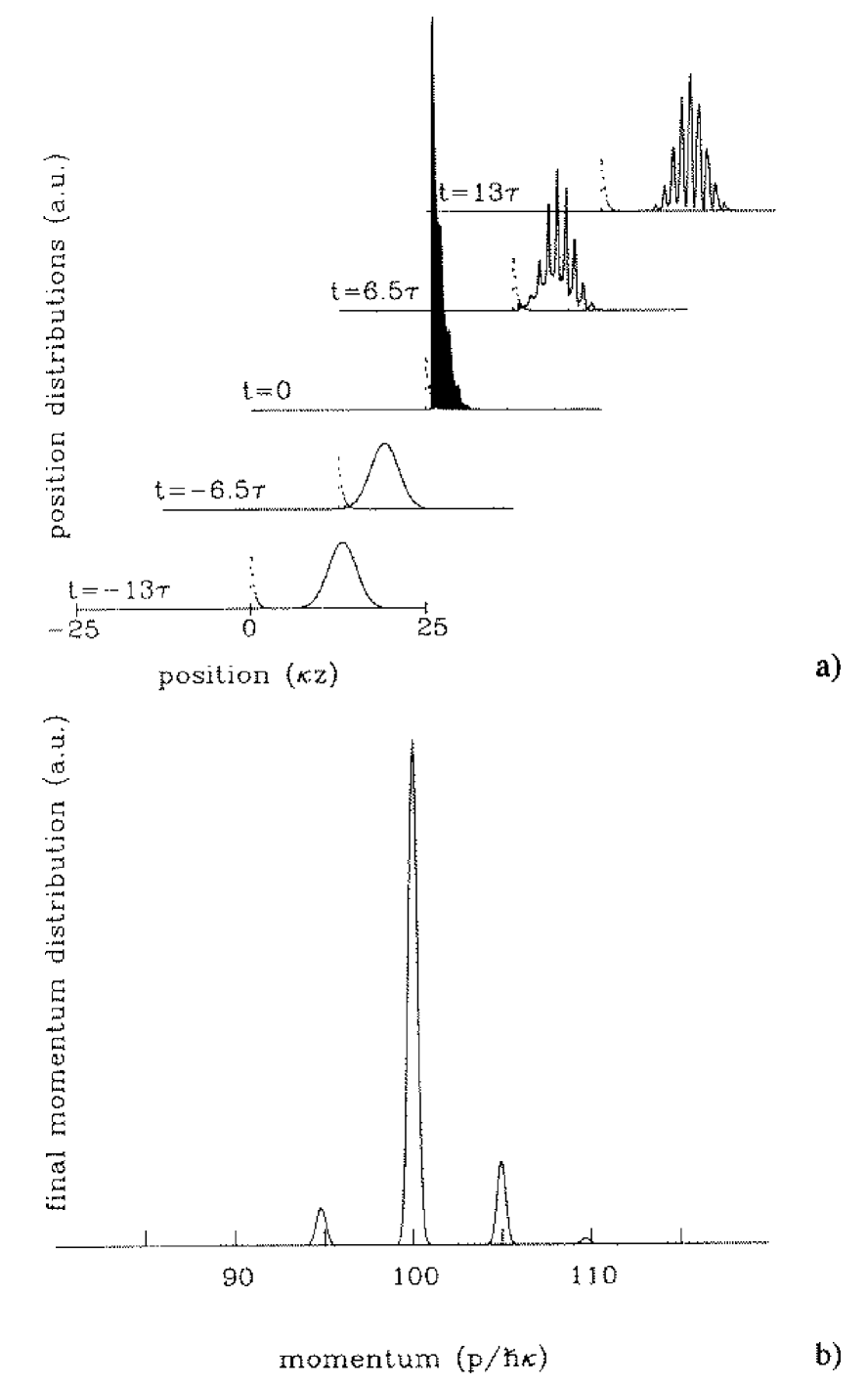
Fig. 3.—: a) Reflection of a wave packet at the modulated mirror. The position distribution at $t=0$ has been cut for the sake of clarity, its actual maximum height is about 15 times the height of the incident wave packet. The parameters used are: initial position $\kappa z_{\rm i}=13$ with standard deviation $\delta\kappa z_{\rm i}=2$, initial momentum $p_{\rm i}=100\>\hbar\kappa$ with standard deviation $\delta p_{\rm i}=0.25\>\hbar\kappa$, modulation frequency $\omega=5/\tau$ so that $q=5\>\hbar\kappa$, modulation depth $\epsilon=1$. b) Final momentum distribution.

We now compare the predictions of this numerical treatment with those of the approach presented in section 4. To this purpose, we consider again the initial Gaussian wave packet:

$$\bar{\psi}(p,0)=\exp\left(-\frac{(p+p_{\rm i})^{2}}{4\delta p_{\rm i}^{2}}\right)\exp\left(-\frac{i}{\hbar}pz_{\rm i}\right).$$ (5.1)

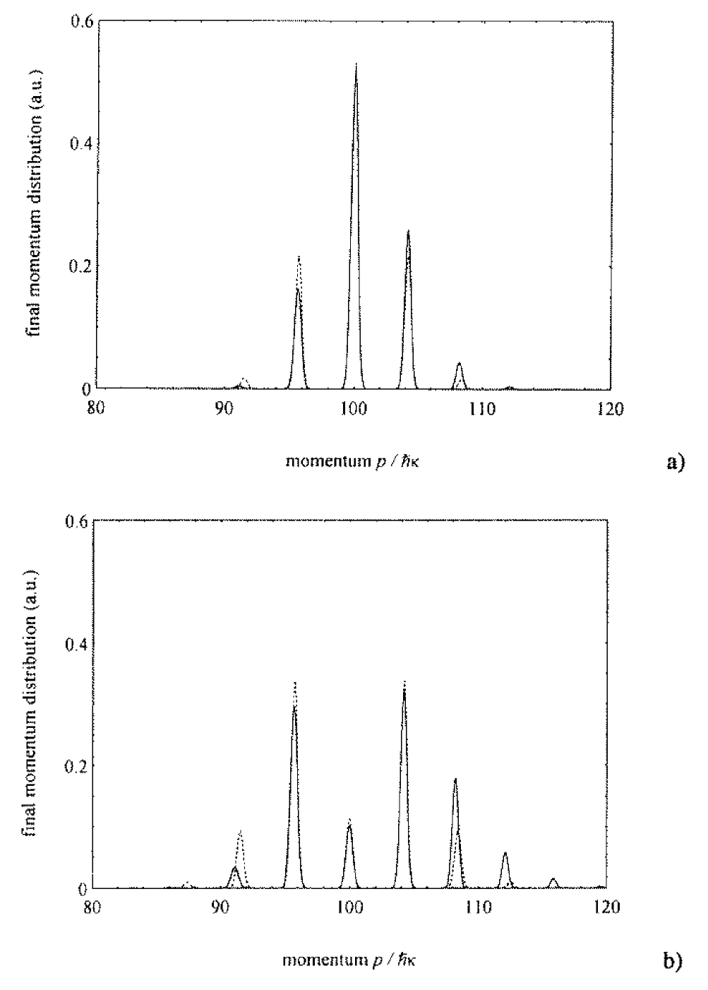
Fig. 4.—: Final momentum distributions, given by the numerical solution (solid line) and the semiclassical approach (dashed line). The parameters used are: initial momentum $p_{\rm i}=100\>\hbar\kappa$, momentum width $\delta p_{\rm i}=0.25\>\hbar\kappa$ (standard deviation), modulation frequency $\omega=4.2/\tau$ (momentum transfer $\Delta p=4.2\>\hbar\kappa$). The situation adopted in (a) (modulation depth $\epsilon=0.6$) maximizes the product of the carrier and first sideband; that in (b)($\epsilon=1$) maximizes the product of the sidebands $n=\pm 1$.

Using the approximate results of section 4, the final wave packet is given by

$$\bar{\psi}(p,t)=\sum_{n}a_{n}{\rm e}^{i\eta}\exp\left(-\frac{(p-nq-p_{\rm i})^{2}}{4\delta p_{\rm i}^{2}}\right)\exp\left(-\frac{i}{\hbar}pz_{\rm i}-\frac{i}{\hbar}\frac{p^{2}t}{2M}\right)$$ (5.2)

where the $a_{n}$ coefficients, given in (4.20), must be evaluated at $p-nq$. The results of the two approaches are shown in figure 4, the solid line for the numerical solution and the dotted line for the semiclassical approximation. The initial wave packet is the same as above. The momentum transfer is $q=4.2\>\hbar\kappa$ and the modulation amplitude $\epsilon$ equals 0.6 (Fig. 4a) and 1 (Fig. 4b). We see that the agreement between the predictions of the two methods is good, although not perfect. In particular, the numerical treatment shows an asymmetry between the heights of the two sidebands $|\bar{\psi}(p_{\rm i}\pm q)|^{2}$, while the approximate treatment predicts equal sideband weights, because of the relation $|J_{n}(x)|=|J_{-n}(x)|$ (see discussion in Sect. 4).

A more systematic comparison of the predictions of this numerical approach with the results derived with the Born approximation and with the semiclassical approach is presented in figure 1. We have determined, for the same initial wave packet as above, and for several values for $q$, the heights of the sidebands $n=\pm 1$. We see that the agreement between the three methods, in their expected range of validity, is quite satisfactory.

6 An atom interferometer.

The vibrating mirror can be used in a number of ways to make an interferometer. In what follows we will consider the case of atoms normally incident on the mirror surface, and making three or more bounces on it. In other words, we rely on the possibility of having a source of slow atoms released above the mirror [23, 24]. With a fast beam of atom, either which could not be reflected at normal incidence, or for which the time to perform repeated bounces is too long, one would need several mirrors — used at grazing incidence if necessary.

Figure 5 illustrates an interferometer based on three consecutive bounces on a vibrating mirror. This is similar in conception to an interferometer constructed from three diffraction gratings [6, 25]. For an incident energy $E_{\rm i}$, we consider two output channels with energies equal to $E_{\rm i}$ and $E_{\rm i}+\hbar\omega$. Each of these two channels can be reached via two paths, which are shown by full lines in figure 5; the other paths, shown dashed in figure 5, do not contribute since we assume that the mirror is “turned off” when these paths hit it.

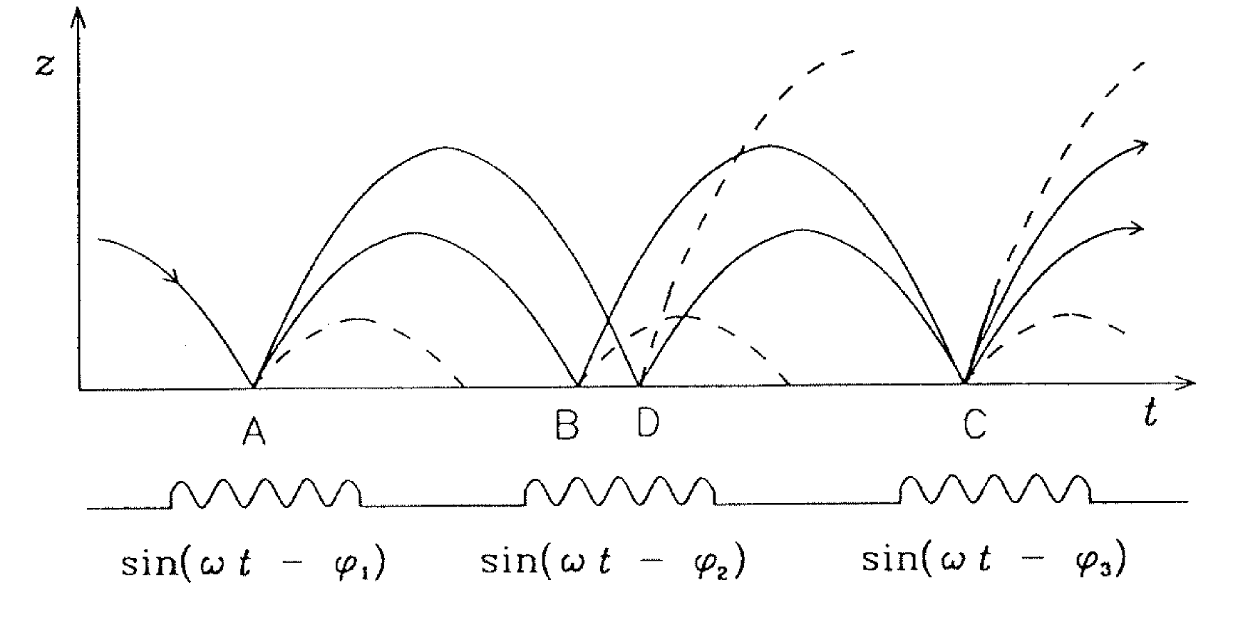
Fig. 5.—: Space-time diagram showing a monochromatic interferometer using three bounces on a vibrating mirror. The paths shown lie at local minima of the classical action. At each reflection, paths corresponding to sidebands of order higher than 1 are omitted for clarity, and paths which return to the mirror when the latter is non-reflecting are shown dashed.

The probability amplitude to exit in a given channel is calculated using the propagators for the region where the atom is in free fall, and the phase shifts corresponding to the interaction with the mirror. The free fall propagator can be evaluated using the integral of the action along the relevant classical paths. We write these in the form $\exp(i\alpha_{AB})$ for the various paths as shown in figure 5. We write $\phi_{m}$ the phase of the mirror vibration at the $m^{\rm th}$ bounce. This phase is dictated purely by the origin in time of the sinusoidal modulation of the mirror for that bounce. Using the expressions (4.20) and (4.21) for the coefficients $a_{n}$ giving the amplitude for transmission into the $n$’th sideband, we now get the two probability amplitudes for transmission into the channels:

$${\cal A}(E_{\rm i}) = a_{0}^{(1)}a_{1}^{(2)}a_{-1}^{(3)}{\rm e}^{i(\phi_{2}-\phi_{3})}{\rm e}^{i(\alpha_{AB}+\alpha_{BC})}$$ (6.1)

$${}+a_{1}^{(1)}a_{-1}^{(2)}a_{0}^{(3)}{\rm e}^{i(\phi_{1}-\phi_{2})}{\rm e}^{i(\alpha_{AD}+\alpha_{DC})}$$

$${\cal A}(E_{\rm i}+\hbar\omega) = a_{0}^{(1)}a_{1}^{(2)}a_{0}^{(3)}{\rm e}^{i\phi_{2}}{\rm e}^{i(\alpha_{AB}+\alpha_{BC})}$$ (6.2)

$${}+a_{1}^{(1)}a_{-1}^{(2)}a_{1}^{(3)}{\rm e}^{i(\phi_{1}-\phi_{2}+\phi_{3})}{\rm e}^{i(\alpha_{AD}+\alpha_{DC})}$$

where the superscript ($m$) indicates the bounce number. For simplicity we have omitted here the contribution of the phases $\eta(p)$ which appear in (4.17). This contribution is the same for the two paths and it cancels out in the final interference pattern.

By choosing a symmetric geometry, we impose the conditions $\alpha_{AB}=\alpha_{DC}$ and $\alpha_{AD}=\alpha_{BC}$ so that the final interferometric phase is given simply by the reflections; it can be written $\theta=\phi_{1}-2\phi_{2}+\phi_{3}$. Note that the other phases associated with the reflections, $q\xi_{\rm eff}$ and, as already noted, $\eta(p)$, exactly cancel out because of the symmetry. In other words all the phases which depend on the incident atomic momentum disappear, and the interferometer will produce high-contrast fringes even when illuminated by a beam of atoms having a broad momentum distribution. The “tradional” three-grating interferometer has the same property. Note also that, for any phase grating including the present one, the $a_{n}$ coefficients satisfy $a_{0}^{*}a_{-1}=-a_{0}a_{1}^{*}$. This ensures that the total probability for ending in one channel or the other, $|{\cal A}(E_{\rm i})|^{2}+|{\cal A}(E_{\rm i}+\hbar\omega)|^{2}$, is independent of the interferometric phase $\theta$.

The fringe amplitude for this interferometer can be written

$${\cal F}=2{\rm Re}\left[(a_{0}a_{1}^{*})^{(1)}(a_{1}a_{-1}^{*})^{(2)}(a_{-1}a_{0}^{*})^{(3)}{\rm e}^{i\theta}\right]$$ (6.3)

This quantity would give ${\cal F}=\cos\theta$ for an ideal interferometer such as a Mach Zehnder. Using the semiclassical approximation (4.20), and denoting $u_{m}$ the index of modulation for the $m$’th bounce, one has

$${\cal F}=2(J_{0}(u_{1})J_{1}(u_{1}))(J_{1}(u_{2}))^{2}(J_{0}(u_{3})J_{1}(u_{3}))\cos\theta$$ (6.4)

This fringe amplitude $\cal F$ is optimised for $u_{1}=u_{3}=1.08$ and $u_{2}=1.84$, and we get $|{\cal F}|_{\rm max}=0.078$. To maximize in these conditions the separation of the interferometer arms we choose $\epsilon_{2}=1$ at the middle bounce, and (4.15) then gives $\epsilon_{1}=\epsilon_{3}\simeq 1.08/1.84\simeq 0.6$ for the first and third bounces. For example, if the initial momentum is $p_{\rm i}=100\>\hbar\kappa$, (4.15) leads to $\Delta p=4.2\>\hbar\kappa$ for these values of the $\epsilon$’s and $u$’s. This gives a good indication of the optimum case: the numerical solution of the Schrödinger equation gives the maximum $|{\cal F}|_{\rm max}\simeq 0.081$ at $\Delta p\simeq 4.2\>\hbar\kappa$, for the same value of $p_{\rm i}$ (see Figs. 4a and 4b). To optimise instead the fringe contrast, one would use the case $|a_{0}|=|a_{1}|$ for the first and third bounces, producing $100\%$ contrast, with a slightly reduced fringe amplitude.

As an example, consider a cesium atom normally incident on an evanescent wave near-resonant with the atomic transition $6S_{1/2}\rightarrow 6P_{3/2}$. Taking $\kappa\simeq 2\pi/852$ nm, the momentum $100\>\hbar\kappa$ corresponds to a velocity of 35 cm/s, and a bounce height of 6 mm, which is readily realisable in practice. The momentum change $4.2\>\hbar\kappa$ is produced with $\omega=2\pi\times 1.7$  MHz. The two interferometer arms are separated in distance by about 0.5 mm, when both are near their maximum height, and in time by about 3 ms (the difference in arrival times at the second bounce). Thus macroscopic path separation can be obtained.

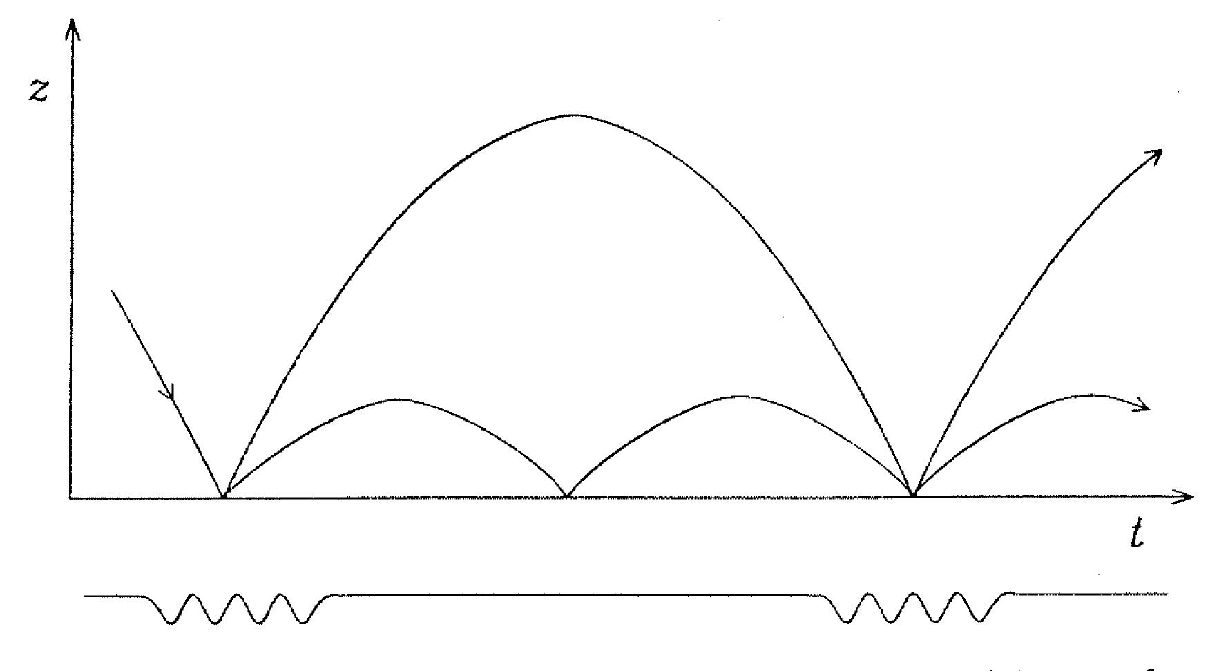
Fig. 6.—: Interferometer design in which the interference phase is sensitive to the acceleration due to gravity. Since the vibrating mirror can only transfer a few $\hbar\kappa$ of momentum, a practical design would involve several bounces before the arms are recombined, as described in the text.

The interference phase will be destroyed not only by mechanical fluctuations of the dielectric surface supporting the evanescent wave, but also by intensity fluctuations of the evanescent wave itself. To estimate the effect of the latter, we note that if the intensity fluctuates by a fraction $\epsilon$, then the effective mirror position (Eq. (4.13)) moves by $\epsilon/2\kappa$. The change produced in the interferometer phase is then $\epsilon p/\hbar\kappa$ radians; this can be understood simply as a higher sensitivity to fluctuations when the de Broglie wavelenght is small, or, equivalently, when the interferometer area is large. One must eliminate not only fluctuations in time but also in the transverse spatial profile of the laser beam forming the evanescent wave “mirror”. To make a flat mirror, one could use a Gaussian laser beam of waist $w$ internally reflected from a concave glass surface of radius of curvature R: when $w=\sqrt{2R/\kappa}$ the glass surface curvature compensates the Gaussian fall-off of the laser beam intensity profile, and the mirror presents a flat reflecting surface for the atoms. A transverse magnetic quadrupole field could help to confine the atom without perturbing the vertical motions of the interferometer arms.

The most obvious first use of the vibrating mirror interferometer is simply to investigate the preservation of coherence during a reflection off the evanescent wave mirror — this could be done by introducing more and more bounces between the splitting and recombining of the two interferometer arms. A second use is as a probe of the acceleration due to gravity. For this, one would not use the symmetric arrangement which we have considered so far, but instead one allows the two arms to bounce many times until they are recombined “automatically” after $m$ (and $m+1$) bounces, where $mp^{\prime}=(m+1)p$, with $p^{\prime 2}=p^{2}+2M\hbar\omega$ (Fig. 6). The mirror is vibrated only for the initial and final bounces; in between it is stationary. For this case, the interferometer phase is dominated by the contributions from the free flights between bounces. One finds that while such an interferometer provides a sensitive probe of the acceleration due to gravity, it is also highly chromatic, producing fringes only for a very small class of incident momenta centred around $p$.

Conclusion.

To summarize, we have presented here the principles of a vibrating mirror for atoms, which constitutes a novel beam splitter for atomic de Broglie waves. We have investigated two analytical theoretical approaches for this new scheme, in order to determine the amplitudes and the phases of the outgoing atomic waves. The results are in excellent agreement with a numerical approach to the problem.

The typical momentum transferred by a vibrating mirror formed with an evanescent light wave is a few photon momenta. Although this is not as large as the transfers obtained by some
other devices, we believe that it should provide, because of its conceptual simplicity, a convenient tool for atom optics and interferometry. Indeed, unlike other atom optics components such as micro-fabricated gratings, it is quite easy to change rapidly (on the microsecond scale) the modulation factor of the light wave forming the mirror. This gives in return a direct control upon the phases and intensities of the diffracted de Broglie waves, and this allows one to conceive simple and useful atomic interferometric devices, such as the ones shown in figures 5 and 6.

References

- [1] Haavig D.L. and Reifenberger R., Phys. Rev. B 26 (1982) 6408
-
[2]
Cook R.J. and Hill R.K., Opt. Commun. 43 (1982) 258;
Balykin V.I., Letokhov V.S., Ovchinnikov Y.B. and Sidorov A.I., Sov. Phys. JETP Lett. 45 (1987) 353 -
[3]
Sokolov Yu.L. and Yakovlev V.P., Sov. Phys. JETP
56 (1982) 7;
Sokolov Yu.L., The Hydrogen Atom, G.F. Bassani, M. Inguscio and T.W. Hänsch Eds. (Springer, Berlin 1989). - [4] Carnal O. and Mlynek J., Phys. Rev. Lett. 66 (1991) 2689.
- [5] Shimizu F., Shimizu K. and Takuma H., Phys. Rev. A 46 (1992) R17
- [6] Keith D.W., Ekstrom C.R., Turchette Q.A. and Pritchard D.E., Phys. Rev. Lett. 66 (1991) 2693.
-
[7]
Kasevich M. and Chu S., Phys. Rev. Lett. 67
(1991) 181;
Kasevich M. and Chu S., Appl. Phys. B 54 (1992) 321. - [8] Weiss D.S., Young B.N. and Chu S., Phys. Rev. Lett. 70 (1993) 2706.
-
[9]
Riehle F., Kisters Th., Witte A., Helmcke J. and Bordé Ch.J.,
Phys. Rev. Lett. 67 (1991) 177;
Riehle F., Witte A., Kisters Th. and Helmcke J., Appl. Phys. B 54 (1992) 333. -
[10]
Sterr U., Sengstock K., Möller J.H., Bettermann D.
and Ertmer W., Appl. Phys. B 54 (1992) 341;
Rieger V., Sengstock K., Sterr U., Möller J.H. and Ertmer W., Opt. Commun. 99 (1993) 172 - [11] Robert J., Miniatura Ch., Le Boiteux S., Reinhardt J., Bocvarski V. and Baudon J., Europhys. Lett. 16 (1991) 29.
- [12] Goldner L.S., Gerz C., Spreeuw R.J.C., Rolston S.L., Westbrook C.I. and Phillips W.D., Phys. Rev. Lett. 72 (1994) 997
- [13] Lawall J. and Prentiss M., Phys. Rev. Lett. 72 (1994) 993.
- [14] Pfau T., Kurtsiefer Ch., Adams C.S., Sigel M. and Mlynek J., Phys. Rev. Lett. 71 (1993) 3427.
- [15] Clauser J.F., Physica B 151 (1988) 262.
- [16] The decay constant of the modulated potential (3.2) may be different from the one of the static potential. In this work, however, we restrict ourselves to identical ’s.
- [17] Henkel C., Courtois J.-Y., Kaiser R., Westbrook C. and Aspect A., Laser Phys. 4 (1994) 1042.
- [18] “Table of Integrals, Series, and Products”, I.S. Gradshteyn and I.M. Ryzhik Eds. (Academic Press Inc., San Diego, 1980) formula 6.576.4.
- [19] Henkel C., Courtois J.-Y. and Aspect A., J. Phys. II France 4 (1994) 1955
- [20] Gradshteyn I.S., op. cit., formula 17.23.19. Note that the formula 17.23.19 has to be normalized correctly.
- [21] Martin P.J., Gould P.L., Oldaker B.G., Miklich A.H. and Pritchard D.E., Phys. Rev. A 36 (1987) 2495
- [22] Press W.H., Flannery B.P., Teukolsky S.A. and Vetterling W.T., Numerical Recipes (Cambridge University Press, Cambridge, 1986).
- [23] Kasevich M.A., Weiss D.S. and Chu S., Opt. Lett. 15 (1990) 607.
- [24] Aminoff C.G., Steane A.M., Bouyer P., Desbiolles P., Dalibard J. and Cohen-Tannoudji C., Phys. Rev. Lett. 71 (1993) 3083.
-
[25]
Colella R., Overhauser A.W. and Werner S.A.,
Phys. Rev. Lett. 34 (1975) 1472;
Golub R. and Lamoureaux S.K., Phys. Lett. A 162 (1992) 122;
Rasel E. et al., Proceedings fo the workshop on “Waves and Particles in Light and Matter”, Trani, 1992 (Plenum Press, 1994) p. 429.