Spatial overlap of nonclassical ultrashort light pulses and formation of polarization-squeezed light

Abstract

We investigate the spatial overlap of nonclassical ultrashort light pulses produced by self-phase modulation effect in electronic Kerr media and its relevance in the formation of polarization-squeezed states of light. The light polarization is treated in terms of four quantum Stokes parameters whose spectra of quantum fluctuations are investigated. We show that the frequency at which the suppression of quantum fluctuations of Stokes parameters is the greatest can be controlled by adjusting the linear phase difference between pulses. By varying the intensity of one pulse one can suppress effectively the quantum fluctuations of Stokes parameters. We study the overlap of nonclassical pulses inside of an anisotropic electronic Kerr medium and we show that the cross-phase modulation effect can be employed to control the polarization-squeezed state of light. Moreover, we establish that the change of the intensity or of the nonlinear phase shift per photon for one pulse controls effectively the squeezing of Stokes parameters. The spatial overlap of a coherent pulse field with an interference pulse produced by mixing two quadrature-squeezed pulses on a beam splitter is analyzed. It is found that squeezing is produced in three of the four Stokes parameters, with the squeezing in the first two being simultaneous.  
PACS: 42.50.Dv, 42.50.Lc.

Keywords: ultrashort light pulses, electronic Kerr nonlinearity, self-phase modulation, cross-phase modulation, polarization-squeezed light.

I Introduction

Quantum states of light with squeezed polarization have recently been in the focus of theoretical and experimental investigations. The quantum analysis of the light polarization is generally based on four Stokes parameters associated with four Hermitian Stokes operators [1, 2]. By definition, the quantum state of light with the level of quantum fluctuations of Stokes operators smaller than the level corresponding to the coherent state is called polarization-squeezed (PS) state. Its existence was predicted theoretically in [3] and was revealed experimentally in a series of recent experiments [4, 5, 6]. Historically, the first experimental realization of a PS state of light implied the mixing of a strong orthogonally-polarized coherent beam with squeezed vacuum on a 50/50 beam splitter (BS) [4]. The optical parametric amplification ($\chi^{2}$) has also been successfully employed to generate the PS state of light [7, 8, 9]. In the last decade the improvement of fiber optics techniques in the pulse field regime facilitated experiments directed to produce nonclassical solitons [10, 11] or highly stable zero-dispersion quadrature-squeezed ultrashort light pulses (USPs) [12, 13, 14]. Recently it has been found experimentally that the simple spatial overlap of two orthogonally polarized quadrature-squeezed pulses leads to the formation of the PS light [5, 6].

The self-phase modulation (SPM) effect, which is responsible for the quadrature squeezing of pulses in optical Keer-like media ($\chi^{3}$), does not influence the photon statistics of pulses since the photon number is a constant of motion [15]. It was noted for the first time in [16], that a consistent time-dependent quantum description of the SPM effect must necessarily account for the additional noise related to nonlinear absorbtion (the imaginary part of nonlinear susceptibility). In [17] the Kerr nonlinearity has been treated as a Raman-like one, the quantum and thermal noises being considered as a fluctuating addition to the relaxation nonlinearity in the interaction Hamiltonian. The addition is necessary in order to preserve the commutation relations among the pulse field-amplitude operators. Hence, the resulting quantum equation of motion for the total field includes the Hermitian-phase noise operator which describes the coupling of the field to a collection of localized, independent, medium oscillators. Besides, the average value of the noise operator on the coherent state is considered to be zero. The time-delayed Raman response of nonlinearity, which is around $50$ fs in fused-silica fibers, varies over frequencies of interest and is caused by back action of nonlinear nuclear vibrations on electronic ones. However, the contribution of Raman oscillators to the Kerr effect is secondary to the one of the electronic motion. Indeed, if we deal with the nonlinear propagation of USPs, for instance through fused-silica fibers, since the Raman oscillators contribute with less than $20\%$ to the Kerr effect, the contribution of the electronic motion on $\sim 1$ fs time scale is more than $80\%$ [18]. The analysis of the SPM effect then has to focus on contribution of the electronic motion, especially in the case of USPs with a duration much less than the time-delayed Raman response or in case the pulse’s frequencies are far from any Raman resonances. An attempt to develop a quantum theory of the pulse SPM primarily due to the electronic motion has been undertaken in [19], but the electronic nonlinearity has been modeled as a Raman-like one. The electronic nonlinear response function in the frequency domain over the bandwidths of interest is considered constant and approximated with a delta function in the time domain. This implies an instantaneous electronic response of the Kerr nonlinearity. In real situations the nonlinear response of electronic nonlinearity is finite. It results in a non-delta relaxation function in the proper analytical description of the Kerr effect. Such a consistent description based on the momentum operator, which is connected with the evolution of the field in space and incorporates the relaxation function of the electronic nonlinearity, has been implemented in [20, 21], where the correlation functions and spectra of quadrature components of USPs subjected to the SPM effect in the electronic Kerr medium are investigated. Since the momentum operator is in the normally ordered form, in order to satisfy the commutation relations for time-dependent Bose operators there is no need for additional fluctuating terms. The approach developed in [20, 21] for the SPM effect has been extended in [22] to the case of two USPs undergoing, besides the SPM effect, the cross-phase modulation (XPM) effect.

In this paper we apply the quantum theory of the SPM and combined SPM-XPM effects developed in [20, 21] and [22], respectively, to the case of spatial overlap and interference on a BS of quadrature-squeezed pulses. The nonclassical USPs are obtained by undergoing the SPM effect in an inertial electronic Kerr medium. The finite relaxation time of the electronic Kerr nonlinearity is accounted for and the dispersion of linear properties is described in the first approximation of the dispersion theory. We show that the approach for the SPM effect based on the momentum operator allows an adequate calculation of correlation functions and fluctuation spectra of quantum Stokes operators.

The paper is organized as follows. In Section II the quantum model of SPM effect for USPs based on the momentum operator for the pulse field is exposed briefly. We present the space-evolution equation for time dependent Bose operators, its solution, as well as some elements of the algebra of Bose operators. Section III introduces the quantum characterization of polarization of light in terms of Stokes operators, as well as their correlation functions and spectra. In Section IV we analyze the overlap between a coherent USP and a quadrature-squeezed one, the latter USP being produced by employing the SPM effect in an electronic isotropic Kerr medium. The average values, the correlation functions of Stokes operators $\hat{S}_{2}$ and $\hat{S}_{3}$ are computed, and the spectrum of $\hat{S}_{2}$ is graphically represented. This analysis is continued in Section V by investigating the spatial overlap of two independent quadrature-squeezed USPs. In Section VI we study the overlap of two quadrature-squeezed pulses inside a nonlinear anisotropic Kerr medium in the presence of the combined SPM-XPM effect. The momentum operator for the XPM effect introduces the section. Here we show that the XPM effect can be employed to control the formation of polarization-squeezed spectra. Section VII is dedicated to the interference on a BS of two independent quadrature-squeezed USPs and their overlap with a coherent USP or with squeezed vacuum. We reveal that the squeezing is possible in three Stokes parameters $\hat{S}_{0}$, $\hat{S}_{1}$, and $\hat{S}_{2}$. We compare our analytical results with the experimental ones reported in [5, 6]. Our concluding remarks are presented in Section VIII.

II SPM effect in electronic Kerr medium

The traditional way to derive the quantum equation for the SPM effect is based on the interaction Hamiltonian. As a consequence one obtains a time-evolution equation. The transition to space-evolution equation is usually realized by enforcing the replacement $t\rightarrow z/u$, where $z$ is the distance passed inside the Kerr medium and $u$ is the group velocity. This approach is reasonable for single-mode radiation. However, the analytical description of the nonlinear pulse propagation contains both $t$ and $z$. The consistent quantum description of the Kerr effect requires then the use of the momentum operator connected with the evolution of the pulse field in space [23].

When accounting for the finite relaxation time of the Kerr nonlinearity the SPM effect is described with the following momentum operator [20, 21, 22]:

$$\hat{G}_{\rm{spm}}(z)=\hbar\beta\int_{-\infty}^{\infty}dt\int_{-\infty}^{t}H(t-t_{1})\hat{\mathbf{N}}\bigl{[}\hat{n}(t,z)\hat{n}(t_{1},z)\bigl{]}dt_{1}$$ (1)

where $\hbar$ is the Plank constant, the factor $\beta$ is defined by the Kerr nonlinearity of the medium ($\beta=\hbar\omega_{0}k_{0}n_{2}/8n_{0}V$ [22, 24]), $\hat{\mathbf{N}}$ is the normal ordering operator, $H(t)$ is the causal nonlinear response function [$H(t)\neq 0$ at $t\geq 0$ and $H(t)=0$ at $t<0$], $\hat{n}(t,z)=\hat{A}^{+}(t,z)\hat{A}(t,z)$ is the “photon number density” operator in the cross-section $z$ of the medium, and $\hat{A}(t,z)$ and $\hat{A}^{+}(t,z)$ are the photon annihilation and creation Bose operators with the commutation relation $[\hat{A}(t_{1},z),\hat{A}^{+}(t_{2},z)]=\delta{(t_{2}-t_{1})}$, respectively. The thermal noise is neglected and the expression (1) is averaged over the thermal fluctuations. In our approach the pulse duration $\tau_{p}$ is much greater than the relaxation time $\tau_{r}$, and the Kerr medium is lossless and dispersionless; that is, the frequencies of the pulse are off resonance.

In Heisenberg representation, the space evolution of $\hat{A}(t,z)$ is given by the equation [23]

$$i\hbar\frac{\partial\hat{A}(t,z)}{\partial z}=\left[\hat{G}_{\rm{spm}}(z),\hat{A}(t,z)\right].$$ (2)

Then, with (1) the space evolution equation of $\hat{A}(t,z)$ in the moving coordinate system ($z=z^{{}^{\prime}}$, $t=t^{{}^{\prime}}-z/u$, where $t^{{}^{\prime}}$ is the running time and $u$ is the group velocity)

$$\frac{\partial\hat{A}(t,z)}{\partial z}-\hat{O}(t)\hat{A}(t,z)=0$$ (3)

has the solution given by

$$\hat{A}(t,z)=e^{\hat{O}(t)}\hat{A}(t),$$ (4)

where $\hat{O}(t)=i\gamma q(\hat{n}(t))$, $\gamma=\beta z$, $\hat{n}(t)=\hat{A}^{+}(t)\hat{A}(t)$ is the “photon number density” operator at the entrance into the medium, $\hat{n}(t)=\hat{n}(t,z=0)$, and $q(\hat{n}(t))=\int_{-\infty}^{\infty}h(t_{1})\hat{n}(t-t_{1})dt_{1}$, with $h(t)=H(|t|)$.

In comparison with the so-called nonlinear Schrödinger equation, used in the quantum theory of optical solitons (see for instance [25] and references therein), in (3) the light pulse dispersion spreading in the medium is absent. This approach corresponds to the first approximation of the dispersion theory [24]. Note that the structure of $q(\hat{n}(t))$ is like that of the linear response in the quantum description of a USP spreading in the second-order approximation.

The statistical features of pulses at the output of the medium can be evaluated by using the algebra of time-dependent Bose operators [20, 21]. For example, in such algebra we have a permutation relation of the form:

$$\hat{A}(t_{1})e^{\hat{O}(t_{2})}=e^{\hat{O}(t_{2})+{\mathcal{D}}(t_{2}-t_{1})}\hat{A}(t_{1})$$ (5)

where ${\mathcal{D}}(t_{2}-t_{1})=i\gamma h(t_{2}-t_{1})$, $2\gamma$ is the nonlinear phase shift per photon. By using the theorem of normal ordering [20, 21] one obtains the average values of the Bose operators over the initial coherent summary state $|\alpha(t)\rangle$:

$$\langle e^{\hat{O}(t)}\rangle = e^{i\phi(t)-\mu(t)},$$ (6)

$$\langle e^{\hat{O}(t_{1})+\hat{O}(t_{2})}\rangle = e^{i\phi(t_{1})+i\phi(t_{2})-\mu(t_{1})-\mu(t_{2})-{\mathcal{K}}(t_{1},t_{2})}.$$ (7)

The parameters $\phi(t)=2\gamma\bar{n}(t)$, $\mu(t)=\gamma^{2}\bar{n}(t)/2$ are connected with SPM of the pulse. Here $\phi(t)$ is the nonlinear phase addition caused by SPM. The eigenvalue $\alpha(t)$ of the annihilation operator $\hat{A}(t)$ over the coherent state $|\alpha(t)\rangle$ can be written as $\alpha(t)=|\alpha(t)|e^{i\varphi(t)}$, where $\varphi(t)$ is the linear phase of the pulse. Then $|\alpha(t)|^{2}=\langle\hat{n}(t)\rangle\equiv\bar{n}(t)$. The time dependence can be separated in $|\alpha(t)|$ by introducing the pulse’s envelope $r(t)$ so that $|\alpha(t)|=|\alpha(0)|r(t)$ with $r(0)=1$. For the simplicity of notations let $\phi(t=0)\equiv\phi_{0}$ and $\bar{n}(t=0)\equiv\bar{n}_{0}$. In (6) and (7) ${\mathcal{K}}(t_{1},t_{2})=\mu_{0}\,r^{2}(t_{1}+\tau/2)g(\tau)$ is the temporal correlator due to SPM, where $\mu_{0}=\gamma\bar{n}_{0}$, $g(\tau)=(1+|\tau|/\tau_{r})h(\tau)$, and $\tau=t_{2}-t_{1}$.

Notice that in our approach there is no assumption about the form of the relaxation function $H(t)$ of the Kerr nonlinearity. It is positive at any instant $t>0$ and zero otherwise. If the SPM efect is due primarily to the electronic motion occurring on $\sim 1$ fs time scale ($\tau_{r}\leq 1$ fs), then in the absence of one- and two-photon and Raman resonances, the relaxation function at $t\geq 0$ can be approximated in the form [24]:

$$H(t)=(1/\tau_{r})\exp{\left(-t/\tau_{r}\right)}.$$ (8)

In the following sections this specific form of the relaxation function is used when evaluating the Fourier transform of $h(\tau)$ and $g(\tau)$.

III Quantum characterization of the light polarization; Stokes operators

The quantum description of the polarization of light is usually done in terms of four Stokes operators $\hat{S}_{\alpha}$ ($\alpha=\overline{0,3\mathstrut}$) [1, 2]. For two spatially overlapping USPs the Stokes operators are introduced as follows:

$$\hat{S}_{0}(t) = \hat{A}^{+}_{1}(t)\hat{A}_{1}(t)+\hat{A}^{+}_{2}(t)\hat{A}_{2}(t)~{}~{}\,=Tr[\hat{D}^{+}_{1}(t)\hat{D}_{1}(t)],$$ (9)

$$\hat{S}_{1}(t) = \hat{A}^{+}_{1}(t)\hat{A}_{1}(t)-\hat{A}^{+}_{2}(t)\hat{A}_{2}(t)~{}~{}\,=Tr[\hat{\sigma}_{3}\hat{D}^{+}_{1}(t)\hat{D}_{1}(t)],$$ (10)

$$\hat{S}_{2}(t) = \hat{A}^{+}_{2}(t)\hat{A}_{1}(t)+\hat{A}^{+}_{1}(t)\hat{A}_{2}(t)~{}~{}\,=Tr[\hat{\sigma}_{1}\hat{D}^{+}_{2}(t)\hat{D}_{1}(t)],$$ (11)

$$\hat{S}_{3}(t) = i[\hat{A}^{+}_{2}(t)\hat{A}_{1}(t)-\hat{A}^{+}_{1}(t)\hat{A}_{2}(t)]=Tr[-\hat{\sigma}_{2}\hat{D}^{+}_{2}(t)\hat{D}_{1}(t)]$$ (12)

where $\hat{\sigma}_{k}$ are Pauli matrices ($k=\overline{1,3\mathstrut}$), and $D$-matrices are:

$$D_{1}(t)=\left(\begin{array}[]{cc}\hat{A}_{1}(t)&0\\ 0&\hat{A}_{2}(t)\\ \end{array}\right),\quad D_{2}(t)=\left(\begin{array}[]{cc}0&\hat{A}_{1}(t)\\ \hat{A}_{2}(t)&0\\ \end{array}\right).$$ (13)

The definition of Stokes operators $\hat{S}_{k}$ in terms of Pauli matrices (10)-(12) suggests that in quantum optics they play a similar role to the Pauli matrices $\hat{\sigma}_{k}$ which in quantum theory of angular momentum describe the rotations in two-spinor formalism. Indeed, apart from a normalization factor, the commutation relations for Stokes operators are identical to those for Pauli matrices; $[\hat{S}_{i}(t),\hat{S}_{j}(t)]=2i\varepsilon_{ijk}\hat{S}_{k}(t)$, where indices $i,j,k=1,2,3$ are taken by cyclic permutations. The energy operator $\hat{S}_{0}(t)$ commutes with any $\hat{S}_{k}(t)$, i.e., $[\hat{S}_{0}(t),\hat{S}_{k}(t)]=0$. In addition, the Stokes operators generate a special non-abelian unitary group of symmetry transformations SU2 that obeys the same Lie algebra as the three-dimensional rotation group of Pauli matrices. Since the Stokes operator $\hat{S}_{0}(t)$ describes the total energy of the two pulse field at the time $t$, $\hat{S}_{k}(t)$ characterize light polarization and form a Cartesian axis system. The polarization state is visualized as a vector on the Poincaré sphere and each point on the sphere corresponds to a definite polarization state whose variation is characterized by the motion of the point on the sphere. If the Stokes vector points in the direction of $\hat{S}_{1}$, $\hat{S}_{2}$, or $\hat{S}_{3}$, than the polarized part of the beam is horizontally, linearly at $45^{\circ}$, or right-circularly polarized, respectively. When Stokes vectors of two USPs point in opposite directions pulses do not interfere. The radius of Poincaré sphere, i.e., the average length of the Poincaré vector ${\mathcal{R}}(t)=(\sum_{k=1}^{3}\langle\hat{S}_{k}(t)\rangle^{2})^{1/2}$, defines the average intensity of the polarized part of the radiation. The ratio of the intensity of the polarized part to the total average intensity $\langle\hat{S}_{0}(t)\rangle$ is called degree of polarization ${\mathcal{P}}(t)={{\mathcal{R}}(t)}/\langle\hat{S}_{0}(t)\rangle$ and it is an important measure in quantum optics.

To analyze the behavior of quantum fluctuations of Stokes operators $\hat{S}_{\alpha}$ we introduce their correlation functions:

$$R_{S_{\alpha}}(t,t+\tau)=\langle\hat{S}_{\alpha}(t)\hat{S}_{\alpha}(t+\tau)\rangle-\langle\hat{S}_{\alpha}(t)\rangle\langle\hat{S}_{\alpha}(t+\tau)\rangle.$$ (14)

In the frame of the quantum model for the SPM effect presented in Section II the correlation functions (14) can be analytically computed by using permutation relations of the type (5) and the averages (6) and (7) of time-dependent Bose operators (see for example [26]). The average values in (14) are calculated on the summary coherent quantum state $|\alpha(t)\rangle=|\alpha_{1}(t)\rangle\otimes|\alpha_{2}(t)\rangle$. We assume here that the initial USPs are in coherent states, the $j$-th pulse’s operator $\hat{A}_{j}(t)$ acting only on the corresponding state vector $|\alpha_{j}(t)\rangle$ within the associated sub-Hilbert space ${{\mathcal{H}}_{j}}$, so the factorization of the quantum states of the two sub-Hilbert spaces takes place. The orthogonal basis of summary states belongs to the global Hilbert space ${\mathcal{H}}={{\mathcal{H}}_{1}}\otimes{{\mathcal{H}}_{2}}$. This basic assumption is followed in the paper when calculating the quantum average of physical quantities of interest. If both USPs are in coherent states, then $R_{S_{\alpha}}(t,t+\tau)=\delta(\tau)$. As is well known from experiments, if USPs undergo some nonlinear transformations (for example, parametric amplification or SPM effect) and further overlap spatially, than the formation of PS state of light is allowed. This means that, in the theoretical description of the formation of the PS state in such processes, the correlation functions of Stokes parameters are different from $\delta$-function. However, the polarization squeezing cannot be obtained in all Stokes parameters at the same time. We show bellow, by analytically deriving the correlation functions of Stokes parameters that the spatial overlap of quadrature-squeezed pulses, the overlap of nonclassical pulses inside an anisotropic Kerr medium in the presence of combined SPM-XPM effect, or the interference of nonclassical USPs on a BS, lead to the formation of the PS state.

With the correlation function calculated in agreement with (14) one can proceed with the evaluation of the spectra $S_{S_{\alpha}}(\omega,t)$ of quantum fluctuations of Stokes operators at any instant $t$ by merely applying the Wiener-Khintchine (WK) theorem, which states that

$$S_{S_{\alpha}}(\omega,t)=\int^{\infty}_{-\infty}R_{S_{\alpha}}(t,t+\tau)e^{i\omega\tau}d\tau.$$ (15)

For two coherent USPs that overlap spatially the spectrum of quantum fluctuations of $\hat{S}_{\alpha}$ is frequency independent and constant, i.e., $S^{coh}_{S_{\alpha}}(\omega,t)=1$. Consequently, the deviation from the coherent level $S^{*}_{S_{\alpha}}(\omega,t)=S_{S_{\alpha}}(\omega,t)-1$ can be used as a measure of quantum fluctuations behavior. Thus, since the case $0<S^{*}_{S_{\alpha}}(\omega,t)$ corresponds to anti-squeezing, the case $-1\leq S^{*}_{S_{\alpha}}(\omega,t)<0$ corresponds to the suppression of quantum fluctuations of $\hat{S}_{\alpha}$.

IV Overlapping coherent and quadrature-squeezed pulses

In the quantum model for the SPM effect in Kerr media developed in [20, 21] and shortly exposed in Section II the finite relaxation time of the electronic nonlinearity is accounted. Note that this approach leads to an accurate calculation of correlation functions and fluctuation spectra of quadrature components for USPs subjected to the combined SPM-XPM effect in electronic Kerr media [22]. Within the quantum model [20, 21] we consider the spatial overlap of a coherent USP ($\hat{A}_{1}(t)$) with a quadrature-squeezed one ($\hat{A}_{2}(t,l)$). The nonclassical USP is obtained by passing a Kerr medium of length $l$ [$\gamma=\beta l$, $\hat{A}_{2}(t,l)=e^{\hat{O}(t)}\hat{A}_{2}(t)$]. The Stokes operators are defined in agreement with (9)-(12) with D-matrices in the form:

$$D_{1}(t)=\left(\begin{array}[]{cc}\hat{A}_{1}(t)&0\\ 0&\hat{A}_{2}(t,l)\\ \end{array}\right),\quad D_{2}(t)=\left(\begin{array}[]{cc}0&\hat{A}_{1}(t)\\ \hat{A}_{2}(t,l)&0\\ \end{array}\right).$$ (16)

We point out that the Kerr effect does not affect the photon statistics [15] and, in the assumption that one can neglect the dispersion effects, the operators $\hat{S}_{0}$ and $\hat{S}_{1}$, as well as their dispersions, are conserved. Below, by investigating the fluctuation spectra, we show that the overlap of USPs produces the squeezing of quantum fluctuations in $\hat{S}_{2}$ or $\hat{S}_{3}$. With the use of Eqs. (4) and (6) we estimate the average values of these operators. We have: $\langle\hat{S}_{0}(t)\rangle=\sum_{i=1}^{2}\bar{n}_{i}(t)$, $\langle\hat{S}_{1}(t)\rangle=\bar{n}_{1}(t)-\bar{n}_{2}(t)$,

$$\langle\hat{S}_{2}(t)\rangle = 2[\bar{n}_{1}(t)\bar{n}_{2}(t)]^{1/2}e^{-\mu_{2}(t)}\cos{[\Phi_{2}(t)-\varphi_{1}(t)]},$$ (17)

$$\langle\hat{S}_{3}(t)\rangle = 2[\bar{n}_{1}(t)\bar{n}_{2}(t)]^{1/2}e^{-\mu_{2}(t)}\sin{[\Phi_{2}(t)-\varphi_{1}(t)]},$$ (18)

where $\Phi_{2}(t)=\phi_{2}(t)+\varphi_{2}(t)$. Note that $\langle\hat{S}_{3}(t)\rangle$ is shifted in phase with $-\pi/2$ in comparison with $\langle\hat{S}_{2}(t)\rangle$, in complete agreement with the Heisenberg uncertainty relation for noncommuting observables. To investigate the behavior of quantum fluctuation of Stokes operators $\hat{S}_{2}$ and $\hat{S}_{2}$ we proceed by evaluating their correlation functions (14). It is not difficult to show that in the approximation $\gamma\ll 1$ by using Eqs. (4)-(7) the correlation function $R_{S_{2}}(t,t+\tau)$ has the following analytical form:

$$R_{S_{2}}(t,t+\tau)=\delta(\tau) + h(\tau)\bar{n}_{1}(t)\phi_{2}(t)\sin{2[\varphi_{1}(t)-\Phi_{2}(t)]}$$ (19)

$$+ g(\tau)\bar{n}_{1}(t)\phi^{2}_{2}(t)\sin^{2}{[\varphi_{1}(t)-\Phi_{2}(t)]}.$$ (20)

With the correlation function (20) the fluctuation spectrum of $\hat{S}_{2}$ can be obtained by applying the WK theorem (15). Allowing for a small change of the envelope $r(t)$ during the relaxation time $\tau_{r}$ and accounting the fact that for the electronic nonlinearity (8) we have: $\int_{-\infty}^{\infty}h(\tau)e^{i\omega\tau}d\tau=2L(\omega)$ and $\int_{-\infty}^{\infty}g(\tau)e^{i\omega\tau}d\tau=4L^{2}(\omega)$ [20, 21, 22], for the fluctuation spectrum of $\hat{S}_{2}$ we finally obtain

$$S_{S_{2}}(\Omega,t)=1 + 2L(\Omega)\bar{n}_{1}(t)\phi_{2}(t)\sin{2[\varphi_{1}(t)-\Phi_{2}(t)]}$$ (21)

$$+ 4L^{2}(\Omega)\bar{n}_{1}(t)\phi^{2}_{2}(t)\sin^{2}{[\varphi_{1}(t)-\Phi_{2}(t)]},$$ (22)

where $L(\Omega)=1/(1+\Omega^{2})$. Here the dimensionless frequency $\Omega=\omega\tau_{r}$ is introduced for the simplicity of notations. The correlation function of $\hat{S}_{3}$, as well as its fluctuation spectrum, can be easily obtained by shifting (20) and (22) in phase with $\pi/2$, respectively. Since the spectral density of quantum fluctuations (22) depends on the relaxation time of the electronic nonlinearity, the latter defines the level of quantum fluctuations below to the one corresponding to the coherent state. The second term on the r.h.s. of Eq. (22), which can be negative for a definite linear phase difference $\Delta\varphi(t)=\varphi_{2}(t)-\varphi_{1}(t)$ between USPs, indicates clearly that the level of quantum fluctuations of $\hat{S}_{2}$ can be less than that corresponding to the coherent state, $S_{S_{2}}^{coh}(\Omega,t)=1$. Let $\Delta\varphi(t)$ at a definite reduced frequency $\Omega_{0}$ has the form

$$\Delta\varphi_{opt}(t)=\frac{1}{2}\arctan{\left(\frac{1}{L(\Omega_{0})\phi_{2}(t)}\right)}-\phi_{2}(t).$$ (23)

Then, at this $\Delta\varphi_{opt}(t)$ the fluctuation spectrum (22) reaches the minimum value

$$S_{S_{2}}(\Omega_{0},t)=1+2\bar{n}_{1}(t)\phi^{2}_{2}(t)L^{2}(\Omega_{0})-2\bar{n}_{1}(t)\phi_{2}(t)L(\Omega_{0})[1+\phi^{2}_{2}(t)L^{2}(\Omega_{0})]^{1/2}.$$ (24)

At any frequency $\Omega$ the fluctuation spectrum writes:

$$S_{S_{2}}(\Omega,t) = S_{S_{2}}(\Omega_{0},t)+2\bar{n}_{1}(t)\phi^{2}_{2}(t)[L^{2}(\Omega)-L^{2}(\Omega_{0})]-2\bar{n}_{1}(t)\phi_{2}(t)[L(\Omega)-L(\Omega_{0})]$$ (26)

$$\times\{1+\phi^{2}_{2}(t)L(\Omega_{0})[L(\Omega)+L(\Omega_{0})]\}[1+\phi_{2}^{2}(t)L^{2}(\Omega)]^{-1/2}$$

As already pointed out, in order to characterize the deviation from the coherent level we introduce the normalized spectral variance $S^{*}_{S_{2}}(\Omega,t)=[S_{S_{2}}(\Omega,t)-1]/\bar{n}_{1}(t)$. In Figs. 1 and 2 we display $S^{*}_{S_{2}}(\Omega,t)$ for different values of the nonlinear phase addition $\phi_{2}(t)$. For linear phase difference optimized at low frequencies $\Omega_{0}=0$ the squeezing in $\hat{S}_{2}$ is maximal around $\Omega\approx 0$ (Fig. 1). In case $\Omega_{0}=1$, the squeezing take place essentially at high frequencies $\Omega\approx 1$ ($\omega=1/\tau_{r}$) (Fig. 2). Thus, the choice of linear phase difference allow us to produce the squeezing basically at the frequency of interest. Moreover, the increase of the nonlinear phase addition $\phi_{2}(t)$ produces a better level of squeezing.

FIG. 1.: Normalized spectral variance $S^{*}_{S_{2}}(\Omega,t)$ for linear phase difference $\Delta\varphi(t)$ chosen optimal at $\Omega_{0}=0$. Curves are calculated at time $t=0$ and correspond to $\phi_{0,2}=0.5$ (a), $\phi_{0,2}=1$ (b), $\phi_{0,2}=2$ (c), $\phi_{0,2}=3$ (d).

FIG. 2.: As in Fig. 1 but for $\Omega_{0}=1$.

V Overlapping quadrature-squeezed pulses

Now we focus our attention to the case of spatial overlap of two independent quadrature-squeezed USPs. The nonclassical pulses obtained at the exits of electronic Kerr media of lengths $l_{1}$ and $l_{2}$ further overlap spatially. The Stokes operators for the nonclassical USPs are defined in agreement with (9)-(12) in terms of annihilation [$\hat{A}_{j}(t,l_{j})=e^{\hat{O}_{j}(t)}\hat{A}_{j}(t)$] and creation [$\hat{A}^{+}_{j}(t,l_{j})=\hat{A}^{+}_{j}(t)e^{\hat{O}^{+}_{j}(t)}$] operators ($j=1,2$) with D-matrices in the form:

$$D_{1}(t)=\left(\begin{array}[]{cc}\hat{A}_{1}(t,l_{1})&0\\ 0&\hat{A}_{2}(t,l_{2})\\ \end{array}\right),\quad D_{2}(t)=\left(\begin{array}[]{cc}0&\hat{A}_{1}(t,l_{1})\\ \hat{A}_{2}(t,l_{2})&0\\ \end{array}\right).$$ (27)

Proceeding as in the previous section for the average value of $\hat{S}_{2}$ and $\hat{S}_{3}$ we have:

$$\langle\hat{S}_{2}(t)\rangle = 2[\bar{n}_{1}(t)\bar{n}_{2}(t)]^{1/2}e^{-\mu_{1}(t)-\mu_{2}(t)}\cos{[\Phi_{2}(t)-\Phi_{1}(t)]},$$ (28)

$$\langle\hat{S}_{3}(t)\rangle = 2[\bar{n}_{1}(t)\bar{n}_{2}(t)]^{1/2}e^{-\mu_{1}(t)-\mu_{2}(t)}\sin{[\Phi_{2}(t)-\Phi_{1}(t)]}.$$ (29)

The correlation function of $\hat{S}_{2}$ calculated by using the relations (4)-(7) in the approximation $\gamma_{j}\ll 1$ is

$$R_{S_{2}}(t,t+\tau)=\delta(\tau) + h(\tau)[\bar{n}_{1}(t)\phi_{2}(t)-\bar{n}_{2}(t)\phi_{1}(t)]\sin{2[\Phi_{1}(t)-\Phi_{2}(t)]}$$ (30)

$$+ g(\tau)[\bar{n}_{1}(t)\phi^{2}_{2}(t)+\bar{n}_{2}(t)\phi^{2}_{1}(t)]\sin^{2}{[\Phi_{1}(t)-\Phi_{2}(t)]}.$$ (31)

Compare the relations (17)-(20) and (28)-(31). Instead of $\varphi_{1}(t)$ we have now $\Phi_{1}(t)=\phi_{1}(t)+\varphi_{1}(t)$ where $\phi_{1}(t)$ is the nonlinear phase addition due to SPM effect on the pulse 1 after passing the Kerr medium of length $l_{1}$. With the WK theorem, for the fluctuation spectrum of $\hat{S}_{2}$ we get:

$$S_{S_{2}}(\Omega,t)=1 + 2L(\Omega)[\bar{n}_{1}(t)\phi_{2}(t)-\bar{n}_{2}(t)\phi_{1}(t)]\sin{2[\Phi_{1}(t)-\Phi_{2}(t)]}$$ (32)

$$+ 4L^{2}(\Omega)[\bar{n}_{1}(t)\phi^{2}_{2}(t)+\bar{n}_{2}(t)\phi^{2}_{1}(t)]\sin^{2}{[\Phi_{1}(t)-\Phi_{2}(t)]}.$$ (33)

Besides adjusting the nonlinear phase differences $\phi_{j}(t)$, we can control the spectral density (33) by changing the intensities $\bar{n}_{j}(t)$ of USPs. If the linear phase difference $\Delta\varphi(t)=\varphi_{2}(t)-\varphi_{1}(t)$ at a definite frequency $\Omega_{0}$ is taken in the form

$$\Delta\varphi_{opt}=\frac{1}{2}\arctan{\left(\frac{\bar{n}_{1}(t)\phi_{2}(t)-\bar{n}_{2}(t)\phi_{1}(t)}{L(\Omega_{0})[\bar{n}_{1}(t)\phi^{2}_{2}(t)+\bar{n}_{2}(t)\phi^{2}_{1}(t)]}\right)}+\phi_{1}(t)-\phi_{2}(t),$$ (34)

then the fluctuation spectrum (33) reaches the minimum value

$$S_{S_{2}}(\Omega_{0},t) = 1+2[\bar{n}_{1}(t)\phi^{2}_{2}(t)+\bar{n}_{2}(t)\phi^{2}_{1}(t)]L^{2}(\Omega_{0})-2L(\Omega_{0})\{[\bar{n}_{1}(t)\phi_{2}(t)-\bar{n}_{2}(t)\phi_{1}(t)]^{2}$$ (35)

$$+ L^{2}(\Omega_{0})[\bar{n}_{1}(t)\phi^{2}_{2}(t)+\bar{n}_{2}(t)\phi^{2}_{1}(t)]^{2}\}^{1/2}.$$ (36)

At any frequency $\Omega$ the fluctuation spectrum is:

$$S_{S_{2}}(\Omega,t)\! = \!S_{S_{2}}(\Omega_{0},t)+2[\bar{n}_{1}(t)\phi^{2}_{2}(t)+\bar{n}_{2}(t)\phi^{2}_{1}(t)][L^{2}(\Omega)-L^{2}(\Omega_{0})]-2[L(\Omega)-L(\Omega_{0})]$$ (37)

$$\times \!\!\{\left[\bar{n}_{1}(t)\phi_{2}(t)-\bar{n}_{2}(t)\phi_{1}(t)\right]^{2}+L(\Omega_{0})[L(\Omega)+L(\Omega_{0})][\bar{n}_{1}(t)\phi^{2}_{2}(t)+\bar{n}_{2}(t)\phi^{2}_{1}(t)]^{2}\}$$ (38)

$$\times \!\!\left\{[\bar{n}_{1}(t)\phi_{2}(t)-\bar{n}_{2}(t)\phi_{1}(t)]^{2}+L^{2}(\Omega_{0})[\bar{n}_{1}(t)\phi^{2}_{2}(t)+\bar{n}_{2}(t)\phi^{2}_{1}(t)]^{2}\right\}^{-1/2}.$$ (39)

In Figs. 3 and 4 we present the normalized spectral variance $S^{*}_{S_{2}}(\Omega,t)=[S^{coh}_{S_{2}}(\Omega,t)-1]/\bar{n}_{1}(t)$ for different relations between pulses intensities. One can see that, by increasing the intensity of the control USP $\mathbf{2}$, we achieve a better level of squeezing.

FIG. 3.: Normalized spectral variance $S^{*}_{S_{2}}(\Omega,t)$ for linear phase difference $\Delta\varphi(t)$ chosen optimal at $\Omega_{0}=0$. Curves are calculated at time $t=0$ with $\phi_{1,0}=2$ and $\gamma_{1}=2\gamma_{2}$ and correspond to $\bar{n}_{2,0}/\bar{n}_{1,0}=1$ (a), $\bar{n}_{2,0}/\bar{n}_{1,0}=2$ (b), $\bar{n}_{2,0}/\bar{n}_{1,0}=3$ (c), $\bar{n}_{2,0}/\bar{n}_{1,0}=5$ (d), $\bar{n}_{2,0}/\bar{n}_{1,0}=7$ (e).

FIG. 4.: As in Fig. 3 but for $\Omega_{0}=1$.

VI Overlapping quadrature-squeezed USPs in anisotropic Kerr media

When two USPs with orthogonal polarization and/or different frequencies overlap spatially inside an anisotropic Kerr medium, beside SPM effect of pulses, the XPM effect and parametric interaction occur. The parametric frequency conversion can be neglected in the assumption of a large phase mismatch $|\Delta|>\rm{min}\{\tilde{\beta}|A_{1}(0)|,\tilde{\beta}|A_{2}(0)|\}$ and $\Delta z\gg 1$ [3, 24]. In this situation the XPM effect can be employed to control the spectra of quantum fluctuations of quadratures [22], as well as those of quantum Stokes parameters [26]. The consistent description of the combined SPM-XPM effect is based on the momentum operator $\hat{G}(z)=\sum_{j=1}^{2}\hat{G}_{\rm{spm}}(z)+\hat{G}_{\rm{xpm}}(z)$ where

$$\hat{G}_{\rm{xpm}}(z)=\hbar\widetilde{\beta}\int_{-\infty}^{\infty}dt\int_{-\infty}^{t}H(t-t_{1})\left[\hat{n}_{1}(t,z)\hat{n}_{2}(t_{1},z)+\hat{n}_{1}(t_{1},z)\hat{n}_{2}(t,z)\right]dt_{1}.$$ (40)

In the above expression $\tilde{\gamma}=\widetilde{\beta}z$ is the nonlinear coupling coefficient [22, 26]. With the total momentum operator $\hat{G}(z)$ we derive the solution of the space-evolution equation (3) for the pulse $\mathbf{1}$;

$$\hat{A}_{1}(t,z)=e^{\hat{O}_{1}(t)+\hat{\tilde{O}}_{2}(t)}\,\hat{A}_{1}(t),$$ (41)

where $\hat{\tilde{O}}_{j}(t)=i\tilde{\gamma}q(\hat{n}_{j}(t))$ includes the contribution due to the XPM effect. The expression for $\hat{A}_{2}(t,z)$ can be derived by changing the indexes $1\leftrightarrow 2$ in (41). The application of the solution (41) requires the use of the extended algebra of time-dependent Bose operators that contains permutation relations of the form

$$\hat{A}_{j}(t_{1})e^{\hat{O}_{j}(t_{2})} = e^{\hat{O}_{j}(t_{2})+{\mathcal{D}}_{j}(t_{2}-t_{1})}\hat{A}_{j}(t_{1}),$$ (42)

$$\hat{A}_{j}(t_{1})e^{\hat{\tilde{O}}_{j}(t_{2})} = e^{\hat{\tilde{O}}_{j}(t_{2})+{\tilde{\mathcal{D}}}(t_{2}-t_{1})}\hat{A}_{j}(t_{1}),$$ (43)

where here ${\tilde{\mathcal{D}}}(t_{2}-t_{1})=i\tilde{\gamma}h(t_{2}-t_{1})$ [22]. With expressions (42)-(43) for the average values of the Bose operators over the initial coherent summary state $|\alpha(t)\rangle$ we get:

$$\langle e^{\hat{O}_{j}(t)}\rangle = e^{i\phi_{j}(t)-\mu_{j}(t)},\quad~{}\langle e^{\hat{\tilde{O}}_{j}(t)}\rangle=e^{i\tilde{\phi}_{j}(t)-\tilde{\mu}_{j}(t)},$$ (44)

$$\langle e^{\hat{O}_{j}(t_{1})+\hat{O}_{j}(t_{2})}\rangle = e^{i[\phi_{j}(t_{1})+\phi_{j}(t_{2})]-[\mu_{j}(t_{1})+\mu_{j}(t_{2})]-{\mathcal{K}}_{j}(t_{1},t_{2})},$$ (45)

$$\langle e^{\hat{\tilde{O}}_{j}(t_{1})+\hat{\tilde{O}}_{j}(t_{2})}\rangle = e^{i[\tilde{\phi}_{j}(t_{1})+\tilde{\phi}_{j}(t_{2})]-[\tilde{\mu}_{j}(t_{1})+\tilde{\mu}_{j}(t_{2})]-\tilde{\mathcal{K}}_{j}(t_{1},t_{2})}.$$ (46)

The parameters $\tilde{\phi}_{j}(t)=2\tilde{\gamma}\bar{n}_{j}(t)$, $\tilde{\mu}_{j}(t)=\tilde{\gamma}^{2}\bar{n}_{j}(t)/2$ are connected with the XPM of the $j$-th pulse. Here $\tilde{\phi}_{j}(t)$ and $\tilde{\mathcal{K}}_{j}(t_{1},t_{2})$ are the nonlinear phase addition and the temporal correlator caused by XPM, respectively.

The Stokes operators are defined in agree with the formulas (9)-(12) with D-matrices in the form:

$$D_{1}(t)=\left(\begin{array}[]{cc}\hat{A}_{1}(t,z)&0\\ 0&\hat{A}_{2}(t,z)\\ \end{array}\right),\quad D_{2}(t)=\left(\begin{array}[]{cc}0&\hat{A}_{1}(t,z)\\ \hat{A}_{2}(t,z)&0\\ \end{array}\right),$$ (47)

where $z$ is the distance inside the anisotropic Kerr medium where the pulses overlap. By using Eqs. (42), (43) and Eq. (44) we estimate the average values of Stokes operators:

$$\langle\hat{S}_{2}(t)\rangle = 2{[\bar{n}_{1}(t)\bar{n}_{2}(t)]}^{1/2}e^{-\Delta_{1}(t)-\Delta_{2}(t)}\cos{[\widetilde{\Phi}_{2}(t)-\widetilde{\Phi}_{1}(t)]},$$ (48)

$$\langle\hat{S}_{3}(t)\rangle = 2{[\bar{n}_{1}(t)\bar{n}_{2}(t)]}^{1/2}e^{-\Delta_{1}(t)-\Delta_{2}(t)}\sin{[\widetilde{\Phi}_{2}(t)-\widetilde{\Phi}_{1}(t)]},$$ (49)

where here $\Delta_{j}(t)=\mu_{j}(t)+\tilde{\mu}_{j}(t)$, $\tilde{\Phi}_{j}(t)=\phi_{j}(t)-\tilde{\phi}_{j}(t)+\varphi_{j}(t)$. In the approximation $\gamma_{j},\tilde{\gamma}\ll 1$, by making use of Eqs. (42), (43) and Eqs. (45), (46), for the correlation function of $\hat{S}_{2}$ we get

$$R_{S_{2}}(t,t+\tau) = \delta(\tau)+h(\tau)[\bar{n}_{1}(t)\phi_{2}(t)-\bar{n}_{2}(t)\phi_{1}(t)]\sin{2[\widetilde{\Phi}_{1}(t)-\widetilde{\Phi}_{2}(t)]}$$ (50)

$$+ g(\tau)\{\bar{n}_{1}(t)[\phi^{2}_{2}(t)\!+\!\tilde{\phi}^{2}_{2}(t)]+\bar{n}_{2}(t)[\phi^{2}_{1}(t)\!+\!\tilde{\phi}^{2}_{1}(t)]\}\sin^{2}{[\widetilde{\Phi}_{1}(t)-\widetilde{\Phi}_{2}(t)]}.$$ (51)

One can easily see that in the absence of XPM, i.e. $\tilde{\phi}_{1}(t)=\tilde{\phi}_{2}(t)=0$, the expression above reduces to the expression (31) of the previous section. To derive the analytical expression of the fluctuation spectrum of $\hat{S}_{2}$ we apply the WK theorem. Thus,

$$S_{S_{2}}(\Omega,t) = 1+2L(\Omega)[\bar{n}_{1}(t)\phi_{2}(t)-\bar{n}_{2}(t)\phi_{1}(t)]\sin{2[\widetilde{\Phi}_{1}(t)-\widetilde{\Phi}_{2}(t)]}$$ (52)

$$+ 4L^{2}(\Omega)\{\bar{n}_{1}(t)[\phi^{2}_{2}(t)\!+\!\tilde{\phi}^{2}_{2}(t)]+\bar{n}_{2}(t)[\phi^{2}_{1}(t)\!+\!\tilde{\phi}^{2}_{1}(t)]\}\sin^{2}{[\widetilde{\Phi}_{1}(t)-\widetilde{\Phi}_{2}(t)]}.$$ (53)

Notice that the XPM effect introduces specific contributions in the fluctuation spectrum [compare (53) with (33)]. Their change allows for an additional control of fluctuation spectrum (see [26]). At the linear phase difference $\Delta\varphi(t)=\varphi_{1}(t)-\varphi_{2}(t)$

$$\Delta\varphi(t)_{\rm opt} = \frac{1}{2}\arctan\left(\frac{\bar{n}_{1}(t)\phi_{2}(t)-\bar{n}_{2}(t)\phi_{1}(t)}{L(\Omega_{0})\Bigl{\{}\bar{n}_{0,1}(t)[\phi^{2}_{2}(t)+\tilde{\phi}^{2}_{2}(t)]+\bar{n}_{2}(t)[\phi^{2}_{1}(t)+\tilde{\phi}^{2}_{1}(t)]\Bigl{\}}}\right)$$ (55)

$$+\phi_{1}(t)-\phi_{2}(t)-\tilde{\phi}_{1}(t)+\tilde{\phi}_{2}(t),$$

optimal at a definite frequency $\Omega_{0}=\omega_{0}\tau_{r}$, the spectrum (53) reaches the minimum

$$S_{S_{2}}(\Omega_{0},t) = 1+2L^{2}(\Omega_{0})\left(\bar{n}_{1}(t)[\phi^{2}_{2}(t)+\tilde{\phi}^{2}_{2}(t)]+\bar{n}_{2}(t)[\phi^{2}_{1}(t)+\tilde{\phi}^{2}_{1}(t)]\right)$$ (58)

$$-2L(\Omega_{0})\Bigl{[}\bigl{[}\bar{n}_{1}(t)\phi_{2}(t)-\bar{n}_{2}(t)\phi_{1}(t)\bigl{]}^{2}$$

$$+L^{2}(\Omega_{0})\Bigl{(}\bar{n}_{1}(t)[\phi^{2}_{2}(t)+\tilde{\phi}^{2}_{2}(t)]+\bar{n}_{0,2}(t)[\phi^{2}_{1}(t)+\tilde{\phi}^{2}_{1}(t)]\Bigl{)}^{2}\Bigl{]}^{1/2}.$$

In Fig. 5 we display the fluctuation spectra of $\hat{S}_{2}$ for different relations between the intensities of pulses. With the increase of intensity of the pulse 2 (the control pulse) a better level of suppression of quantum fluctuations can be achieved. A similar result, now displayed in Fig. 6, can be obtained by increasing the nonlinear coefficient $\gamma_{2}$ in comparison with $\gamma_{1}$. In conclusion, besides the optimal linear phase arrangement (55) that produce the suppression of quantum fluctuation at the frequency of interest, the increase of the intensity of the control pulse (Fig. 5), or of the nonlinear coefficient $\gamma_{2}$ (Fig. 6), can be employed for the achievement of desired level of squeezing.

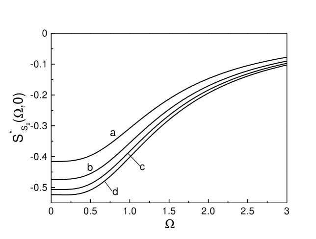
FIG. 5.: Normalized spectral variance $S^{*}_{S_{2}}(\Omega,t)$ at $\phi_{0,1}=2$ for initial phase difference $\Delta\varphi(t)$ chosen optimal at $\Omega_{0}=0$. Curves are calculated at time $t=0$, $\gamma_{1}=\gamma_{2}/4=2\tilde{\gamma}$, and correspond to $\bar{n}_{0,2}=\bar{n}_{0,1}/4$ (a), $\bar{n}_{0,2}=\bar{n}_{0,1}/2$ (b), $\bar{n}_{0,2}=\bar{n}_{0,1}$ (c), $\bar{n}_{0,2}=3\bar{n}_{0,1}$ (d) (from Ref. [26]).

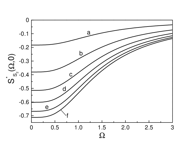
FIG. 6.: Normalized spectral variance $S^{*}_{S_{2}}(\Omega,t)$ at $\phi_{0,1}=2$ for initial phase difference $\Delta\varphi(t)$ chosen optimal at $\Omega_{0}=0$. Curves are calculated at time $t=0$, $\bar{n}_{0,1}=\bar{n}_{0,2}$, $\tilde{\gamma}=\gamma_{1}/2$ and correspond to $\gamma_{2}=2\gamma_{1}$ (a), $\gamma_{2}=3\gamma_{1}$ (b), $\gamma_{2}=4\gamma_{1}$ (c), $\gamma_{2}=5\gamma_{1}$ (d), $\gamma_{2}=6\gamma_{1}$ (e), $\gamma_{2}=7\gamma_{1}$ (f) (from Ref. [26]).

VII Interfering quadrature-squeezed pulses

In this section we show that by overlapping a coherent pulse with an interference USP, obtained by mixing two quadrature-squeezed USPs on a BS, one can produce the simultaneous squeezing in the first two Stokes parameters $\hat{S}_{0}$ and $\hat{S}_{1}$, as well as the squeezing in one of the last two, $\hat{S}_{2}$ or $\hat{S}_{3}$. We shall compare our theoretical results with the experimental ones presented in [5, 6]. We start by analyzing the situation depicted in Fig. 7.

FIG. 7.: Interference on a BS of two independent quadrature-squeezed pulses produced by using the SPM effect in nonlinear electronic Kerr media ($\chi^{(3)}$). The outgoing nonclassical pulse at the output 1 ($\hat{B}_{1}(t)$) is overlapped spatially with a coherent pulse field ($\hat{A}_{3}(t)$).

Two quadrature-squeezed USPs fall simultaneously on an inclined BS with reflectivity $R$ and transmissivity $T$, giving rise to reflected and transmitted interference USPs whose amplitudes depends on $R$ and $T$. The outgoing nonclassical interference USP at the exit 1 of BS ($\hat{B}_{1}(t)$) overlaps with a third coherent USP ($\hat{A}_{3}(t)$). We consider $R$ and $T$ being independent on frequency, direction of propagation or polarization and we treat both reflections symmetrically. In this latest case the relationship between input and output states on BS reads [27]:

$$\left(\begin{array}[]{c}\hat{B}_{1}(t)\\ \hat{B}_{2}(t)\\ \end{array}\right)=\left(\begin{array}[]{cc}i\sqrt{R}&\sqrt{T}\\ \sqrt{T}&i\sqrt{R}\\ \end{array}\right)\left(\begin{array}[]{c}\hat{A}_{1}(t,l_{1})\\ \hat{A}_{2}(t,l_{2})\\ \end{array}\right),$$ (59)

where $\hat{B}_{j}(t)$ is the annihilation operator on the output j of the BS and $\hat{A}_{j}(t,l_{j})=e^{\hat{O}_{j}(t)}\hat{A}_{j}(t)$ ($j=1,2$). The Stokes operators at the output 1 are defined in agree with the formulas (9)-(12) when now the D-matrices are

$$D_{1}(t)=\left(\begin{array}[]{cc}\hat{B}_{1}(t)&0\\ 0&\hat{A}_{3}(t)\\ \end{array}\right),\quad D_{2}(t)=\left(\begin{array}[]{cc}0&\hat{B}_{1}(t)\\ \hat{A}_{3}(t)&0\\ \end{array}\right).$$ (60)

By using the algebra of time-dependent Bose operators developed in [20, 21], and summarily exposed in Section II, for the average values of Stokes parameters on the summary coherent state $|\alpha(t)\rangle$ we find:

$$\langle\hat{S}_{0,1}(t)\rangle = R\bar{n}_{1}(t)+T\bar{n}_{2}(t)\pm\bar{n}_{3}(t)$$ (61)

$$+ 2\sqrt{RT}[\bar{n}_{1}(t)\bar{n}_{2}(t)]^{1/2}e^{-\mu_{1}(t)-\mu_{2}(t)}\sin{[\Phi_{2}(t)-\Phi_{1}(t)]},$$ (62)

$$\langle\hat{S}_{2}(t)\rangle = 2\sqrt{T}[\bar{n}_{2}(t)\bar{n}_{3}(t)]^{1/2}e^{-\mu_{2}(t)}\cos{[\varphi_{3}(t)-\Phi_{2}(t)]}$$ (63)

$$+ 2\sqrt{R}[\bar{n}_{1}(t)\bar{n}_{3}(t)]^{1/2}e^{-\mu_{1}(t)}\sin{[\varphi_{3}(t)-\Phi_{1}(t)]},$$ (64)

where in (62) the sign ‘$+$’ stands for $\langle\hat{S}_{0}(t)\rangle$ and ‘$-$’ for $\langle\hat{S}_{1}(t)\rangle$. The average value of $\hat{S}_{3}$ can be easily obtained by shifting (64) in phase with $-\pi/2$. Notice the appearance of the sin-term in (62) due particularly to the interference on BS. We calculate now the correlation functions of Stokes parameters in the approximation $\gamma_{j}\ll 1$ ($j=1,2$). Below we write down the results obtained in the frame of the quantum model presented in Section II;

$$R_{S_{0,1}}(t,t+\tau) = \delta(\tau)-h(\tau)\{2\sqrt{RT}[\bar{n}_{1}(t)\bar{n}_{2}(t)]^{1/2}[R\phi_{1}(t)\pm T\phi_{2}(t)]\cos{[\Phi_{1}(t)-\Phi_{2}(t)]}$$ (66)

$$~{}~{}~{}~{}~{}~{}~{}~{}~{}~{}~{}~{}~{}~{}~{}~{}+RT[\bar{n}_{1}(t)\phi_{2}(t)-\bar{n}_{2}(t)\phi_{1}(t)]\sin{2[\Phi_{1}(t)-\Phi_{2}(t)]}\}$$

$$+ g(\tau)\{RT[n_{1}(t)\phi^{2}_{2}(t)+n_{2}(t)\phi^{2}_{1}(t)]\cos^{2}{[\Phi_{1}(t)-\Phi_{2}(t)]}\},$$ (67)

$$R_{S_{2}}(t,t+\tau) = \!\delta(\tau)\!+h(\tau)n_{3}(t)\{R\phi_{1}(t)\sin{2[\Phi_{1}(t)\!-\!\varphi_{3}(t)]}\!-\!T\phi_{2}(t)\sin{2[\Phi_{2}(t)\!-\!\varphi_{3}(t)]}\}$$ (68)

$$+ g(\tau)n_{3}(t)\{R\phi^{2}_{1}(t)\cos^{2}{[\Phi_{1}(t)-\varphi_{3}(t)]}+T\phi^{2}_{2}(t)\sin^{2}{[\Phi_{2}(t)-\varphi_{3}(t)]}\}.$$ (69)

The presence of the additional terms besides $\delta$-function indicates that the formation of the PS state in all three Stokes parameters $\hat{S}_{0}$, $\hat{S}_{1}$, $\hat{S}_{2}$ is permitted. The fluctuation spectra are straightforward with the use of WK theorem:

$$S_{S_{0,1}}(\Omega,t) = 1-2L(\Omega)\{2\sqrt{RT}[\bar{n}_{1}(t)\bar{n}_{2}(t)]^{1/2}[R\phi_{1}(t)\pm T\phi_{2}(t)]\cos{[\Phi_{1}(t)-\Phi_{2}(t)]}$$ (71)

$$~{}~{}~{}~{}~{}~{}~{}~{}~{}~{}~{}~{}~{}~{}~{}~{}+RT[\bar{n}_{1}(t)\phi_{2}(t)-\bar{n}_{2}(t)\phi_{1}(t)]\sin{2[\Phi_{1}(t)-\Phi_{2}(t)]}\}$$

$$+ 4L^{2}(\Omega)\{RT[n_{1}(t)\phi^{2}_{2}(t)+n_{2}(t)\phi^{2}_{1}(t)]\cos^{2}{[\Phi_{1}(t)-\Phi_{2}(t)]}\},$$ (72)

$$S_{S_{2}}(\Omega,t) = 1+2L(\Omega)\bar{n}_{3}(t)\{R\phi_{1}(t)\sin{2[\Phi_{1}(t)-\varphi_{3}(t)]}\!-\!T\phi_{2}(t)\sin{2[\Phi_{2}(t)-\varphi_{3}(t)]}\}$$ (73)

$$+ 4L^{2}(\Omega)\bar{n}_{3}(t)\{R\phi^{2}_{1}(t)\cos^{2}{[\Phi_{1}(t)-\varphi_{3}(t)]}\!+\!T\phi^{2}_{2}(t)\sin^{2}{[\Phi_{2}(t)-\varphi_{3}(t)]}\}.$$ (74)

Since the correlation function of $\hat{S}_{3}$ and its fluctuation spectrum can be easily obtained by shifting (69) and (74) in phase with $\pi/2$, respectively, their analytical expression are not presented here. Notice that the above correlation functions and the fluctuation spectra are determined by the parameters $R$ and $T$. In what follows we consider the most common case of a $50/50$ BS, i.e., $R=T=1/2$.

We analyze now the first two Stokes parameters $\hat{S}_{0}$ and $\hat{S}_{1}$ by addressing the issue concerning the optimization of the linear phase difference $\Delta\varphi(t)=\varphi_{1}(t)-\varphi_{2}(t)$. However, due to the analytical complexity of the expression (72), we restrict to the case $\bar{n}_{1}(t)\phi_{2}(t)=\bar{n}_{2}(t)\phi_{1}(t)$ when sin-term in (72) vanishes. Thus, the resulting expression can be minimized if the linear phase difference $\Delta\varphi(t)$ at a defined frequency $\Omega_{0}$ has the form

$$\Delta\varphi^{(\pm)}_{opt}(t)=\arccos{\left[\frac{R\bar{n}_{1}(t)\pm T\bar{n}_{2}(t)}{2[\bar{n}_{1}(t)+\bar{n}_{2}(t)]\phi(t)L(\Omega_{0})}\left(\frac{\bar{n}_{1}(t)}{RT\bar{n}_{2}(t)}\right)^{1/2}\right]}-\phi_{1}(t)+\phi_{2}(t).$$ (75)

With this adjustment (75) for the linear phase difference between pulses the expressions (72) achieve the minimal value

$$S_{S_{0,1}}(\Omega_{0},t)=1-[R\bar{n}_{1}(t)\pm T\bar{n}_{2}(t)]^{2}\,[\bar{n}_{1}(t)+\bar{n}_{2}(t)]^{-1}.$$ (76)

Thus, at any frequency $\Omega$ the spectra (72) take the form

$$S_{S_{0,1}}(\Omega,t)=S_{S_{0,1}}(\Omega_{0},t)+\frac{[R\bar{n}_{1}(t)\pm T\bar{n}_{2}(t)]^{2}}{\bar{n}_{1}(t)+\bar{n}_{2}(t)}\frac{[L(\Omega)-L(\Omega_{0})]^{2}}{L^{2}(\Omega_{0})}.$$ (77)

The fluctuation spectra of $\hat{S}_{0}$ and $\hat{S}_{1}$ for various relations between pulses intensities, at $\Delta\varphi(t)$ optimized at $\Omega_{0}=0$, are displayed in Fig. 8 and 9, respectively. We conclude that the adjustment of the control pulse intensity can be employed to obtain a desired level of squeezing of quantum fluctuations in $\hat{S}_{0}$ and $\hat{S}_{1}$. This conclusion remain also valid in case the linear phase difference is optimized at frequency $\Omega_{0}=1$, the simultaneous suppression being correspondingly achieved at high frequencies $\Omega\approx 1$ ($\omega\approx 1/\tau_{r}$) [Figs. 10 and 11]. With the simplification introduced by the condition $\bar{n}_{1}(t)\phi_{2}(t)=\bar{n}_{2}(t)\phi_{1}(t)$, while the suppression achieved in $\hat{S}_{0}$ is large, the one achieved in $\hat{S}_{1}$ is small.

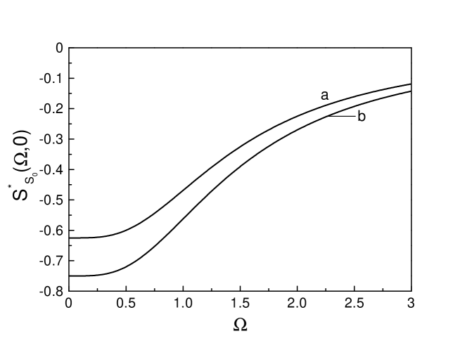
FIG. 8.: Normalized spectral variance $S^{*}_{S_{0}}(\Omega,t)$ for linear phase difference $\Delta\varphi(t)$ chosen optimal at $\Omega_{0}=0$. Curves are calculated at time $t=0$, $R=T=0.5$ and correspond to $\bar{n}_{2,0}=1.5\,\bar{n}_{1,0}$ (a), $\bar{n}_{2,0}=2\,\bar{n}_{1,0}$ (b).

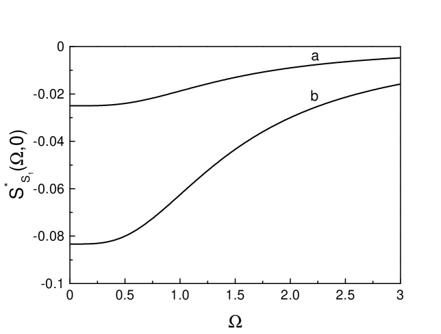
FIG. 9.: Normalized spectral variance $S^{*}_{S_{1}}(\Omega,t)$ for linear phase difference $\Delta\varphi(t)$ chosen optimal at $\Omega_{0}=0$. Curves are calculated at time $t=0$, $R=T=0.5$ and correspond to $\bar{n}_{2,0}=1.5\,\bar{n}_{1,0}$ (a), $\bar{n}_{2,0}=2\,\bar{n}_{1,0}$ (b).

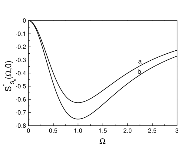
FIG. 10.: As in Fig. 8 but for $\Omega_{0}=1$.

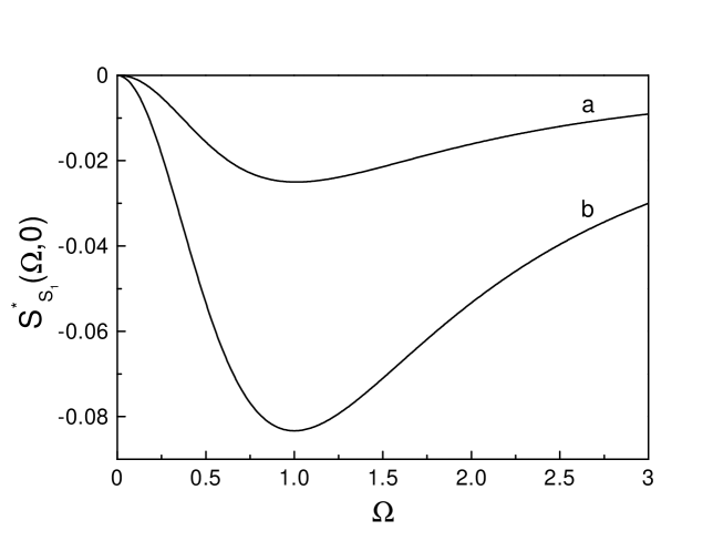
FIG. 11.: As in Fig. 9 but for $\Omega_{0}=1$

However, it is important to remark that in the correlation functions and fluctuation spectra of $\hat{S}_{0}$ and $\hat{S}_{1}$ there is no information about the third coherent USP. As a consequence, the coherent USP can be disregarded in this respect or can be replaced with coherent vacuum which have an uncertainty identical to that of the coherent state. Basically, it means that the outgoing interference USP is already with squeezed quantum fluctuations in $\hat{S}_{0}$ and $\hat{S}_{1}$ before the overlap with the coherent pulse. This situation due to the quantum interference is basically exploited experimentally in [5] where coherent vacuum is mixed on a polarization BS with a quadrature-squeezed USP obtained by using the SPM effect in an optical Kerr fiber ($\chi^{3}$). Indeed, the outgoing interference USP shows the squeezed quantum fluctuations of about $-3.7$ and $-3.6$ dB in $\hat{S}_{0}$ and $\hat{S}_{1}$, respectively. The simultaneous polarization squeezing of about $-3.4$ dB in both $\hat{S}_{0}$ and $\hat{S}_{1}$ is also present when two quadrature-squeezed pulses interfere on a polarization BS [5, 6]. A similar squeezing effect of about $-3$ dB in $\hat{S}_{0}$ and $\hat{S}_{1}$ was reported in [8] where two bright quadrature-squeezed pulses obtained by employing the optical parametrical amplification ($\chi^{2}$) are mixed on a $50/50$ BS.

Let us now consider the next two Stokes parameters $\hat{S}_{2}$ and $\hat{S}_{3}$. We focus on the parameter $\hat{S}_{2}$ since once the suppression of quantum fluctuations is realized in it, the parameter $\hat{S}_{3}$ becomes anti-squeezed, and viceversa. The fluctuation spectrum of Stokes parameter $\hat{S}_{2}$ can be easily minimized in the case $\phi_{1}(t)=\phi_{2}(t)\equiv\phi(t)$ and $\varphi_{1}(t)-\varphi_{2}(t)=\pi/2$. Actually, it was noticed experimentally in [9] that this relative phase of $\pi/2$ is critical for the detection of squeezing. The linear phase difference $\Delta\varphi(t)=\varphi(t)-\varphi_{3}(t)$ that at a defined frequency $\Omega_{0}$ fulfills the condition

$$\cos{2[\phi(t)+\Delta\varphi(t)]}=(R-T)\phi(t)L(\Omega_{0})\sin{2[\phi(t)+\Delta\varphi(t)]}$$

minimizes the expression (74). At this optimal linear phase difference the fluctuation spectrum becomes

$$S_{S_{2}}(\Omega_{0},t)=1+2\bar{n}_{3}(t)\phi^{2}(t)L^{2}(\Omega_{0})-2\bar{n}_{3}(t)\phi(t)L(\Omega_{0})[1+(R-T)^{2}\phi^{2}(t)L^{2}(\Omega_{0})]^{1/2}$$ (78)

In consequence, at any phase $\Omega$ the normalized spectra is

$$S_{S_{2}}(\Omega,t) = S_{S_{2}}(\Omega_{0},t)+2\bar{n}_{3}(t)\phi^{2}(t)[L^{2}(\Omega)-L^{2}(\Omega_{0})]+2\bar{n}_{3}(t)\phi(t)[L(\Omega)-L(\Omega_{0})]$$ (79)

$$\times \{1+(R-T)^{2}\phi^{2}(t)L(\Omega_{0})[L(\Omega)+L(\Omega_{0})]\}[1+(R-T)^{2}\phi^{2}(t)L^{2}(\Omega_{0})]^{-1/2}.$$ (80)

In Fig. 12 we displayed the fluctuation spectrum of $\hat{S}_{2}$ at time moment $t=0$ for different values of the nonlinear phase $\phi(t=0)\equiv\phi_{0}$.

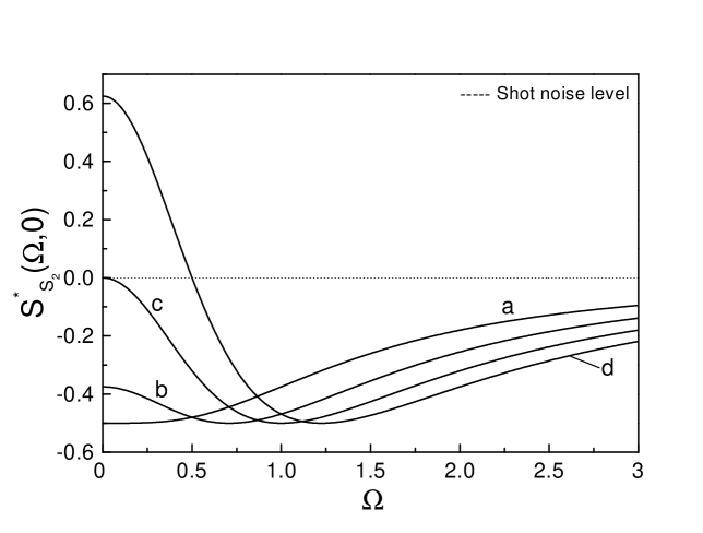
FIG. 12.: Normalized spectral variance $S^{*}_{S_{2}}(\Omega,t)$ for linear phase difference $\Delta\varphi(t)$ chosen optimal at $\Omega_{0}=0$. Curves are calculated at time $t=0$, $R=T=0.5$ and correspond to $\phi_{0}=0.5$ (a), $\phi_{0}=0.75$ (b), $\phi_{0}=1$ (c), $\phi_{0}=1.25$ (d).

The increase of $\phi_{0}$ does not produce a better level of squeezing but moves the squeezing from low frequencies $\Omega\approx 0$ to high frequencies $\Omega\approx 1$. At the same time the squeezing at low frequencies is deteriorating.

Note the obtained suppression of quantum fluctuations due to the stable spatial overlap of two quadrature-squeezed pulses of about of $-2.8$ dB in $\hat{S}_{2}$ reported in [5, 6]. Indeed, since the parameter $\hat{S}_{2}$ becomes squeezed, the parameter $\hat{S}_{3}$ is detected anti-squeezed with about $+23.5$ dB above the shot noise level.

Summarizing, the mixing of two quadrature-squeezed pulses on a $50/50$ BS followed by the spatial overlap of the outgoing interference pulse with a coherent field permits the simultaneous squeezing of quantum fluctuations in the first two Stokes parameters $\hat{S}_{0}$ and $\hat{S}_{1}$, as well as the squeezing in one of the remaining two, $\hat{S}_{2}$ or $\hat{S}_{3}$ (here $\hat{S}_{2}$).

VIII Conclusion

In this work we applied the quantum model developed in [22] to analyze the spatial overlap and interference of quadrature-squeezed USPs. We showed that the spatial overlap of coherent and quadrature-squeezed pulses or of two quadrature-squeezed USPs obtained by employing the SPM effect in the Kerr medium produces the squeezing in one of the last two Stokes parameters $\hat{S}_{2}$ or $\hat{S}_{3}$. We revealed that the adjustment of linear phase difference between pulses leads to the suppression of quantum fluctuations of $\hat{S}_{2}$ or $\hat{S}_{3}$ at the frequency of interest. Moreover, we found that the increase of the intensity of the control USP produces a better level of squeezing.

By investigating the spatial overlap of nonclassical pulses in a nonlinear anisotropic Kerr medium in the presence of XPM effect we established that the increase of the intensity of the control pulse or of one nonlinear coefficient ($\gamma_{2}$) in comparison with the another one ($\gamma_{1}$) is able to realize the desired level of squeezing in $\hat{S}_{2}$ or $\hat{S}_{3}$.

We studied the overlap of a coherent pulse with a nonclassical pulse produced by interfering two quadrature-squeezed USPs on a beam splitter. By studying the fluctuation spectra of Stokes parameters we showed that the nonclassical pulse exhibits the simultaneous squeezing of quantum fluctuations in $\hat{S}_{0}$ and $\hat{S}_{1}$. Besides, we found that its spatial overlap with a coherent pulse field produce the squeezing in $\hat{S}_{2}$ or $\hat{S}_{3}$.

REFERENCES

- [1] Agarwal G. S. and Puri R. R., Phys. Rev. A, 40, 1989 (5179).
- [2] Tanas R. and Kielich S., J. Mod. Opt., 37, 1990 (1935).
- [3] Chirkin A. S., Orlov A. A., and Paraschuk D. Yu., Kvant. Elektron., 20, 1993 (999) (Moscow) [Sov. J. Quantum Electron., 23, 1993 (870)].
- [4] Hald J., Sørensen J. L., Schori C., and Polzik E. S., J. Mod. Opt., 47, 2001 (2599).
- [5] Heersnik J., Gaber T., Lorenz S., Glöckl O., Korolkova N. V., and Leuchs G., Phys. Rev. A, 68, 2003 (013815) (quant-ph/0302100).
- [6] Glöckl O., Heersnik J., Korolkova N. V., Leuchs G., and Lorenz S., J. Opt. B Quantum Semiclass. Opt., 5, 2003 (S492).
- [7] Grangier P., Slusher R. E., Yurke B., and LaPorta A., Phys. Rev. Lett., 59, 1987 (2153).
- [8] Bowen W. P., Treps N., Schnabel R., and Lam P. K., Phys. Rev. Lett., 89, 2002 (253601) (quant-ph/0110129).
- [9] Bowen W. P., Treps N., Schnabel R., Ralph C. T., and Lam P. K. J. Opt. B: Quantum Semiclass. Opt., 5, 2003 (S467).
- [10] Rosenbluh M. and Shelby R. M., Phys. Rev. Lett., 66, 1991 (153).
- [11] Margalit M., Yu C. X., Ippen E. P., and Haus A. H., Opt. Express, 2, 1998 (72).
- [12] Bergman K. and Haus A. H. Opt. Lett., 16, 1991 (663).
- [13] Bergman K., Doerr C. R., Haus A. H., and Shirasaki M., Opt. Lett., 18, 1993 (643).
- [14] Bergman K., Haus A. H., Ippen E. P., and Shirasaki M., Opt. Lett., 19, 1994 (290).
- [15] Kitagawa M. and Yamamoto Y., Phys. Rev. A, 34, 1986 (3974).
- [16] Blow K. J., Loudon R., and Phoenix S. J. D., J. Opt. Soc. Am. B, 8, 1991 (1750).
- [17] Boivin L., Kärtner F. X., and Haus H. A., Phys. Rev. Lett., 73, 1994 (240).
- [18] Joneckis L. G. and Shapiro J. H., J. Opt. Soc. Am. B, 10, 1993 (1102).
- [19] Boivin L., Phys. Rev. A, 52, 1994 (754).
- [20] Popescu F. and Chirkin A. S., Pis’ma Zh. Éksp. Teor. Fiz., 69, 1999 (481), JETP Lett., 69, 1999 (516).
- [21] Chirkin A. S. and Popescu F., J. Russ. Laser Res., 22, 2001 (354).
- [22] Popescu F. and Chirkin A. S., J. Opt. B: Quantum Semiclass. Opt., 4, 2002 (184).
- [23] Toren Mooki and Ben-Aryeh Y., Quantum Opt., 9, 1994 (425).
- [24] Akhmanov S. A., Vysloukh V. A., and Chirkin A. S., Optics of Femtosecound Laser Pulses, 1992 , AIP, New York [Supplemented translation of Russian original, 1988, Nauka, Moscow].
- [25] König F., Zielonka M. A., and Sizmann A. Phys. Rev. A, 66, 2002 (013812).
- [26] Popescu F., Europhys. Lett., 65, 2004 (27).
- [27] Ou Z. Y., Hong C. K., and Mandel L., Optics Communications, 63, 1987 (118).