Environment as a Witness: Selective Proliferation of Information and Emergence of Objectivity in a Quantum Universe

Abstract

We study the role of the information deposited in the environment of an open quantum system in course of the decoherence process. Redundant spreading of information — the fact that some observables of the system can be independently “read-off” from many distinct fragments of the environment — is investigated as the key to effective objectivity, the essential ingredient of “classical reality”. This focus on the environment as a communication channel through which observers learn about physical systems underscores importance of quantum Darwinism — selective proliferation of information about “the fittest states” chosen by the dynamics of decoherence at the expense of their superpositions — as redundancy imposes the existence of preferred observables. We demonstrate that the only observables that can leave multiple imprints in the environment are the familiar pointer observables singled out by environment-induced superselection (einselection) for their predictability. Many independent observers monitoring the environment will therefore agree on properties of the system as they can only learn about preferred observables. In this operational sense, the selective spreading of information leads to appearance of an objective “classical reality” from within quantum substrate.

I Introduction

Emergence of a classical reality within the quantum Universe has been the focus of discussions on the interpretation of quantum theory ever since its inception. Measurement — the process through which we learn about the world — has the power to transform fuzzy quantum states into solid classical facts. Understanding measurements has been therefore rightly regarded as the key to unlocking the mystery of the quantum-classical transition since the early days Wheeler and Zurek (1983). Bohr’s interpretation proposed in 1928 Bohr (1928) introduced the classical domain “by hand”, with a demand that much of the Universe — including measuring devices — must be classical. This Copenhagen interpretation proved to be workable and durable, but is ultimately unsatisfying, because of the arbitrary split between “the quantum” and “the classical”. Thus, Copenhagen interpretation notwithstanding, attempts to explain the emergence of the classical, objective reality (including measurement outcomes) using only quantum theory were made ever since its structure became clear in the late 1920’s.

Von Neumann von Neumann (1955) introduced a particularly influential model of the measurement process. In his approach — and in contrast to Bohr’s view — the apparatus ${\mathcal{A}}$ is also quantum. “Bit-by-bit measurement” Zurek (1981) is the simplest example: a 2-dimensional system ${\mathcal{S}}$ in pure state $\alpha|0\rangle+\beta|1\rangle$ interacts with a 2-dimensional apparatus initially in state $|\mu_{0}^{\mathcal{A}}\rangle$. In course of the controlled-not (or “measurement”) gate the apparatus becomes — as one would now say — entangled with the system ${\mathcal{S}}$:

$$(\alpha|0\rangle+\beta|1\rangle)\otimes|\mu_{0}^{\mathcal{A}}\rangle\rightarrow\alpha|0\rangle\otimes|\mu_{0}^{\mathcal{A}}\rangle+\beta|1\rangle\otimes|\mu_{1}^{\mathcal{A}}\rangle.$$ (1)

This is pre-measurement. It implies correlation of ${\mathcal{S}}$ and ${\mathcal{A}}$, but does not yield a definite outcome.

The structure of Eq. (1) suggests a relative state interpretation of quantum theory Everett III (1957). However, to make contact with the familiar reality, one must point out the “preferred relative states”. Yet, in the bipartite setting of the pre-measurement, such proposals are difficult to make without some ad hoc assumptions (e.g, about the special role of either “memory states” Everett III (1957) or of the “Schmidt basis” Zeh (1973)).

Presence of entanglement in the state obtained after the pre-measurement implies a basis ambiguity — correlation of observables of ${\mathcal{A}}$ with incompatible sets of pure states of the system which cannot be resolved without some modification of the model Zurek (1981). For example, the states $\{|\mu_{0}^{\mathcal{A}}\rangle,|\mu_{1}^{\mathcal{A}}\rangle\}$ of ${\mathcal{A}}$ are in one-to-one correspondence with the states $\{|0\rangle,|1\rangle\}$ of ${\mathcal{S}}$, while the states $\left\{(|\mu_{0}^{\mathcal{A}}\rangle\pm|\mu_{1}^{\mathcal{A}}\rangle)/\sqrt{2}\right\}$ are in one-to-one correspondence with the states $\left\{(\alpha|0\rangle\pm\beta|1\rangle)/\sqrt{2}\right\}$ of ${\mathcal{S}}$. Thus, von Neumann’s model does not account for the existence of a fixed “menu” of possible measurement outcomes — an issue that must be addressed before the apparent selection of one position on this menu (i.e. the “collapse of the wave-packet”) is contemplated.

Decoherence theory (see e.g.  Zurek (1991); Giulini et al. (1996); Paz and Zurek (2001); Zurek (2003a); Schlosshauer (2004) for reviews) added a new element that goes well beyond the von Neumann’s measurement model: in addition to ${\mathcal{S}}$ and ${\mathcal{A}}$, decoherence recognizes the role of the environment ${\mathcal{E}}$ that surrounds ${\mathcal{A}}$ and interacts with the apparatus (or with any other object immersed in ${{\mathcal{E}}}$). The resulting “openness” of ${\mathcal{A}}$ invalidates the egalitarian principle of superposition: while all states in the Hilbert space of the apparatus ${\mathcal{A}}$ are “legal” quantum superpositions, only some of them will retain their identity — will be stable in spite of the coupling to ${\mathcal{E}}$.

Returning to our example, the environment may interact with ${\mathcal{A}}$ in such a way that an arbitrary superposition $\xi_{0}|\mu_{0}^{\mathcal{A}}\rangle+\xi_{1}|\mu_{1}^{\mathcal{A}}\rangle$ is transformed into a mixture $|\xi_{0}|^{2}|\mu_{0}^{\mathcal{A}}\rangle\!\langle\mu_{0}^{\mathcal{A}}|+|\xi_{1}|^{2}|\mu_{1}^{\mathcal{A}}\rangle\!\langle\mu_{1}^{\mathcal{A}}|$ after a very short time. Thus, only the two states $|\mu_{0}^{\mathcal{A}}\rangle$ and $|\mu_{1}^{\mathcal{A}}\rangle$ remain pure over time. Selection of such preferred set of states is known as environment-induced superselection, or einselection. The persistence of the correlation between ${\mathcal{A}}$ and ${\mathcal{S}}$ is the desired prerequisite of measurements, and only stable pointer basis of ${\mathcal{A}}$ selected by the interaction with ${\mathcal{E}}$ fits the bill Zurek (1981, 1982); Paz and Zurek (2001); Zurek (2003a); Schlosshauer (2004). Indeed, after the decoherence time, the joint state of ${\mathcal{S}}$ and ${\mathcal{A}}$, Eq. (1), becomes mixed:

$$|\alpha|^{2}|0\rangle\!\langle 0|\otimes|\mu_{0}^{\mathcal{A}}\rangle\!\langle\mu_{0}^{\mathcal{A}}|+|\beta|^{2}|1\rangle\!\langle 1|\otimes|\mu_{1}^{\mathcal{A}}\rangle\!\langle\mu_{1}^{\mathcal{A}}|.$$ (2)

As a consequence of decoherence, only classical correlations of ${\mathcal{A}}$ with the system states $\{|0\rangle,|1\rangle\}$ persist.

Understanding the reason for the loss of validity of the quantum principle of superposition is a significant step in the understanding of the quantum-classical transition, but it does not go all the way in justifying objectivity: the einselected pointer states are still ultimately quantum. Thus, they remain sensitive to direct measurements — a purely quantum problem. An observer trying to find out about the system directly will generally disturb its state, unless he happens to make a non-demolition measurement Caves et al. (1980); Braginsky and Khalili (1996) in the pointer basis. As a consequence, it is effectively impossible for an initially ignorant observer — someone who does not know what are the pointer states of the system — to find out the state of a physical system through a direct measurement without perturbing it: immediately after a direct measurement the state will be what the observer finds out it is, but not — in general — what it was before.

The situation becomes even more worrisome when one considers many initially ignorant observers attempting to find out about the system. As a consequence of the disturbance caused by a direct measurement on the system, the information gained by the first observer’s measurement can get invalidated by the second observer’s measurement, etc., unless they all happen to measure commuting observables — or more precisely, unless the measured observables share the system’s pointer states as eigenstates.

Quantum subjectivity is to be contrasted with the objectivity of classical physics, where many ignorant observers can — at least in principle — find out the state of the system without modifying it. This is because classical systems admit an underlying objective description (“classical reality”), and classical states can be found out by initially ignorant observers. This is generally not the case for quantum systems. Thus, objective information about quantum systems can be acquired directly by many only by a constrained set of pre-agreed measurements on ${\mathcal{S}}$ (see e.g. Grangier (2002); Poulin (2005)).

Of course — as noted in past discussions of einselection Zurek (1991, 1993, 1998) — there are good reasons for the observers to focus on the set of states singled out by decoherence: only such pointer states of ${\mathcal{S}}$ (or their dynamically evolved descendants) continue to faithfully describe the system in spite of its interaction with ${\mathcal{E}}$. All other states are affected by ${\mathcal{E}}$, making loss of predictability inevitable. Predictability is characteristic of the states of classical systems, and is thus a symptom of a classical reality. But, above all, prediction is the reason for measurements. One can therefore understand how observers with practical experience with the emergent classicality (imposed in our Universe by einselection) will be forced to choose the same pointer observables as they make their choice of what to measure: save for pointer observables, there is no other choice if measurements are to be useful for prediction. This may look like a “pre-agreement”, but it involves no consultation between observers: competing with the environment is simply not an option.

In effect, the environment acts as a superobserver, monitoring the same pointer observable over and over, with frequency and accuracy that cannot be matched by other (e.g., human) observers. They all have to measure observables that commute with the pointer observable. Last but not least, interactions available to observers are similar in structure (e.g., depend on distance, etc.) to the interactions responsible for the einselection Zurek (1998, 2003a). So, predictive utility in presence of decoherence and limited choice of the Hamiltonians available in our Universe motivate “pre-agreement” by constraining measurements to pointer observables. However, even if such “pre-agreement imposed by einselection” can help single out what observables can become objective, the actual role of the environment in what happens in practice far more dramatic and decisive: the environment is not just a superobserver — it becomes a witness. Observers use it to find out about systems of interest. Hence, they must be content with the information that can be extracted from its fragments (as, generally, they will never be able to intercept all of ${\mathcal{E}}$).

In its original formulation, decoherence theory treats the information transferred to ${\mathcal{E}}$ as inaccessible. However, in the real world, this is typically not the case. Indeed, as was pointed out by one of us some time ago Zurek (1993, 1998, 2000), the fact that we gain most of our information by intercepting a small fraction of the photon environment is significant for the emergence of effectively classical states from the quantum substrate. The purpose of this paper is to investigate the consequences of such an indirect information acquisition for the quantum-classical transition, and to explore the relation of this “environment as a witness” Zurek (2003a) point of view to the predictability of the pointer states as well as to other issues raised and partially explored in Ollivier et al. (2004). We shall demonstrate that the manner in which the information is stored in the environment is the reason for the inevitable consensus among many observers about the state of the effectively classical (but ultimately quantum) systems. In other words, the structure of information deposition in ${\mathcal{E}}$ is responsible for the emergence of the objective classical reality from the quantum substrate.

We shall also begin to explore quantum Darwinism: the dynamics responsible for the proliferation of correlations that leads to the survival of the fittest information. This is a natural complement to the environment as a witness approach that is focused on how the data about ${\mathcal{S}}$ can be extracted by interrogating ${\mathcal{E}}$. Quantum Darwinism allows the environment to act as a witness Zurek (2003a); Ollivier et al. (2004); Zurek (2003b), adding a new dimension to the modern decoherence-based view of the emergence of the classical.

In the next section, we propose an operational notion of objectivity and discuss how we will use it to investigate the quantum-classical transition. Sections III and IV set up the notation and introduce tools of information theory required for the present study. Section V contains the core information-theoretic analysis of the manuscript. There, we establish a number of facts about the structure of the information stored in the environment, and study consequences of redundant imprinting of selected system observables in ${\mathcal{E}}$. These general properties are then illustrated in Section VI on a dynamical model used extensively in the study of decoherence. This allows us to extend the results of our analysis, and establish a direct connection between einselection and the emergence of an objective classical reality. Finally, we consider some open questions in Section VII and conclude in Section VIII with a summary.

II Operational definition of objectivity

Quantum Darwinism Zurek (2003a); Ollivier et al. (2004) aims to show that a consensus about the properties of a quantum system — the key symptom of classical reality — arises naturally and inevitably from within quantum theory when one recognizes the role of the environment as a broadcasting medium that acquires — in the process of monitoring the system of interest that leads to decoherence and einselection — multiple copies of the information about preferred properties of the system of interest.

We will set up a rigorous operational framework for the analysis of the emergence of objective classical reality of quantum systems, based on the following definition of objectivity:

Definition II.1 (Objective property)

A property of a physical system is objective when it is

1. simultaneously accessible to many observers,

2. who are able to find out what it is without prior knowledge about the system of interest, and

3. who can arrive at a consensus about it without prior agreement.

This operational definition of what is objective is inspired by the notion of “element of physical reality” used by Einstein, Podolsky and Rosen in their famous “EPR” paper Einstein et al. (1935) on entanglement: “If, without in any way disturbing a system, we can predict with certainty (i.e. with probability equal to unity) the value of a physical quantity, then there exists an element of physical reality corresponding to this physical quantity. […] Regarded not as a necessary, but merely as a sufficient condition of reality, this criterion is in agreement with classical as well as quantum-mechanical ideas of reality.” Any property of the system fulfilling this requirement would be considered an element of objective reality according to the definition we adopt.

The environment as a witness approach recognizes that in our everyday acquisition of data, the decision of what to measure on ${\mathcal{S}}$ is taken out of our hands by the environment, and rests with the dynamics responsible for decoherence — i.e. for the monitoring of the system by ${\mathcal{E}}$. Nevertheless, in the absence of any structure of ${\mathcal{E}}$, this would still be insufficient to explain the emergence of a consensus about the state of ${\mathcal{S}}$. Measurements on the environment suffer from the same basis ambiguity problems as direct measurements on the system: they can be performed in arbitrary bases. Moreover, they generally disturb the state of the environment, and hence, the correlations between ${\mathcal{S}}$ and ${\mathcal{E}}$. Unless all observers had agreed to measure the environment in the same basis, their subsequent measurements on the environment might not yield consensus about the system, and one would not be able to attribute “objective properties” to its state.

The solution to this puzzle becomes obvious after a close inspection of how we learn about systems in the real world. Not only do the independent observers gather information about ${\mathcal{S}}$ indirectly by measuring the environment, but different observers have access to disjoint fragments of ${\mathcal{E}}$. By definition, when the same information about ${\mathcal{S}}$ can be discovered from different fragments, it must have been imprinted in the environment redundantly. In addition, when many disjoint fragments of the environment contain information about the state of the system, its properties can be found out by different observers without the danger of invalidating each other’s conclusions. This is because observables acting on disjoint fragments of ${\mathcal{E}}$ always commute with each other. Hence, the first two requirements for objectivity are satisfied.

Moreover, and this is a crucial result of our study, we will demonstrate that redundant imprinting in the environment selects a preferred set of system observables. In particular, for obvious reasons WZ82a the environment-promoted amplification of information required to arrive at a redundant imprinting cannot amount to cloning. Amplification comes at the price of singling out commuting system observables. As a consequence, even initially ignorant observers performing arbitrary measurements on their fragments of ${\mathcal{E}}$ will find out only about this unique observable. Selectivity of amplification establishes that redundant imprinting in the environment is a sufficient requirement for the emergence of classical objective reality. Thus, the state of the system is de facto objective when its complete and redundant imprint can be found in ${\mathcal{E}}$.

Quantum Darwinism makes novel use of information theory by focusing on the communication capacity of the environment. This approach complements the conventional “system-based” treatments of decoherence. There, the environment is above all an “information sink”, a source of decoherence responsible for irreversible loss of information Zurek (1981); Zurek et al. (1993); Giulini et al. (1996); Paz and Zurek (2001). However, these two complementary approaches do agree in their conclusions: as we will show, the pointer observables singled out by einselection are the only ones that can leave a redundant imprint on the environment. In part, this can be understood as a consequence of the ability of the pointer states to persist while immersed in the environment. Moreover, in both approaches predictability of the preferred states of the system (i.e., either from initial conditions, or from many independent observations on ${\mathcal{E}}$) is the key criterion. This predictability is tied to the resilience that allows the information about the pointer observables to proliferate, very much in the spirit of the “survival of the fittest”, and corroborates conjectures about the role of quantum Darwinism in the emergence of objectivity we have described before Ollivier et al. (2004); Zurek (2003a, b).

III Definitions and conventions

In the setting we are considering, a system ${\mathcal{S}}$ with Hilbert space ${\mathcal{H}}^{\mathcal{S}}$ interacts with an environment ${\mathcal{E}}$ with Hilbert space ${\mathcal{H}}^{\mathcal{E}}$. We denote the dimension of these state spaces by $d^{\mathcal{S}}$ and $d^{\mathcal{E}}$ respectively. Furthermore, we assume that the environment is composed of $N$ environmental subsystems ${\mathcal{E}}_{1},{\mathcal{E}}_{2},\ldots{\mathcal{E}}_{N}$ (see Fig. 1). That is, its Hilbert space has a natural tensor product structure ${\mathcal{H}}^{\mathcal{E}}=\bigotimes_{k=1}^{N}{\mathcal{H}}^{{\mathcal{E}}_{k}}$. This partition plays an important role in our analysis, as it suggests a natural definition of the independently accessible fragments of ${\mathcal{E}}$. We will comment on it at the end of Section IV.

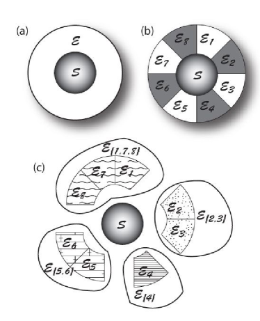
Figure 1: The role and the structure of the environment in decoherence and in quantum Darwinism. (a) Decoherence treats environment as a monolithic entity inaccessible to observers. The only role of ${\mathcal{E}}$ is to be a “sink” of information about ${\mathcal{S}}$. This is enough to understand einselection — the emergence of the preferred pointer observable in the system, with decoherence - free pointer eigenspaces. In our Universe (b) environments are typically not monolithic. Rather, they consist of subsystems, e.g. atoms or photons. From the point of view of decoherence, there is no difference between the paradigms illustrated by (a) and (b): The same environment will lead to the same evolution of the system (e.g., in quantum Brownian motion the same environment can be modeled either as a monolithic field or as a collection of harmonic oscillators). Quantum Darwinism (c) recognizes that observers acquire their information about ${\mathcal{S}}$ without interacting with it directly – from the imprints left by ${\mathcal{S}}$ on the fragments of ${\mathcal{E}}$. Such fragments are generally much smaller than ${\mathcal{E}}$. The central result of this paper is to show that the selected information about the system that is inscribed redundantly — in many copies — on the environment, and can be therefore found out independently from different fragments of ${\mathcal{E}}$ by many observers, concerns the einselected pointer observable.

The joint quantum state of ${\mathcal{S}}$ and ${\mathcal{E}}$ is described by the density operator $\rho^{{\mathcal{S}}{\mathcal{E}}}$ defined on ${\mathcal{H}}^{\mathcal{S}}\otimes{\mathcal{H}}^{\mathcal{E}}$. The reduced state of the system is obtained by “tracing out” the environment $\rho^{\mathcal{S}}=\mathrm{Tr}_{\mathcal{E}}\{\rho^{{\mathcal{S}}{\mathcal{E}}}\}$. It will often be useful to consider the joint state of the system and a fragment of the environment. Such fragment — i.e. a subset of ${\mathcal{E}}=\{{\mathcal{E}}_{1},{\mathcal{E}}_{2},\ldots,{\mathcal{E}}_{N}\}$ — will be denoted by ${\mathcal{F}}$. The reduced state of ${\mathcal{S}}$ and ${\mathcal{F}}$ is obtained by tracing out the complement of ${\mathcal{F}}$: $\rho^{{\mathcal{S}}{\mathcal{F}}}=\mathrm{Tr}_{\overline{\mathcal{F}}}\{\rho^{{\mathcal{S}}{\mathcal{E}}}\}$, where $\overline{\mathcal{F}}={\mathcal{E}}-{\mathcal{F}}$.

Following textbook quantum mechanics, we call “observable of ${\mathcal{S}}$” (resp. of ${\mathcal{E}}$) any Hermitian operator defined on ${\mathcal{H}}^{\mathcal{S}}$ (resp. ${\mathcal{H}}^{\mathcal{E}}$). By convention, we will use the first letters of the alphabet ${\bf A},{\bf B},{\bf C}$ to denote system observables while the last letters ${\bf X},{\bf Y},{\bf Z}$ will be reserved for environment observables. Hermitian operators can be written in their spectral decomposition, e.g.:

$${\bf A}=\sum_{j}a_{j}A_{j}.$$ (3)

Adding to our convention, observables are denoted by bold capital letters, their eigenvalues by lowercase letters, and spectral projectors by capital letters. Only the spectral projectors are of interest to us as they completely characterize the measurement process, and the correlations between observables. We note that as we shall deal with Hermitean observables, coherent states that are the approximate pointer states in many situations of interest (e.g, in underdamped harmonic oscillators) are beyond the scope of our study.

We will use the words “system” and “environment” in a very broad sense. Without loss of generality, we will suppose that ${\mathcal{H}}^{\mathcal{S}}$ is the part of the Hilbert space of ${\mathcal{S}}$ containing the degrees of freedom of interest. Even when the system is macroscopic, e.g. a baseball, we are typically only interested in a few of its degrees of freedom, e.g. center of mass, local densities, etc. Moreover, the degrees of freedom of ${\mathcal{S}}$ that do not couple to ${\mathcal{E}}$ (directly or indirectly) play no role in our analysis. Hence $d^{\mathcal{S}}$ can remain reasonably small even for fairly large systems: $d^{\mathcal{S}}$ is really the number of relevant distinct physical configurations of ${\mathcal{S}}$. This considerably simplifies the notation without compromising the rigor of our analysis.

Similarly, it is not necessary to incorporate “all the rest of the Universe” in ${\mathcal{E}}$. $N$ really counts the number of environmental subsystems that may have been influenced by the system: only they may contain information about ${\mathcal{S}}$. Hence, in many situations — such as a photon environment scattering off an object — the “size” of relevant ${\mathcal{E}}$ can grow over time.

IV Information

The approach to classicality outlined above is based on the existence of correlations between ${\mathcal{S}}$ and its environment that can be exploited by various observers to find out about the system. As both ${\mathcal{S}}$ and ${\mathcal{E}}$ are quantum systems, quantum information theory may appear to be the right tool to study these correlations. This avenue has been considered in the past Zurek (2000, 2003a) in parallel with the approach we pursue here and in Ollivier et al. (2004) and is currently also under investigation Blume-Kohout and Zurek . However, the emphasis here is on the observables, and information about them is easier to characterize through the relevant hypothetical measurements. As in Ollivier et al. (2004), we focus on what can actually be found out about various observables of the system by monitoring observables in fragments of the environment.

The core question we ask is: how much does one learn about observable ${\bf A}$ by measuring a different observable ${\bf X}$? This question has an operational meaning. An observer may be considering measurement of the observable ${\bf A}$, but cannot predict its outcome with certainty. To reduce his ignorance, he can choose to measure a different observable ${\bf X}$. By doing so, he may decrease his uncertainty about the value of ${\bf A}$. The amount by which his uncertainty decreases is precisely the information gain we are going to study. It represents the average number of bits required to write down, in the most efficient way, the relevant data about ${\bf A}$ acquired through the measurement of ${\bf X}$.

We will mostly be interested in the case where ${\bf A}$ acts on the system and ${\bf X}$ acts on a fragment of the environment — which automatically implies that $[{\bf A},{\bf X}]=0$. However, we will occasionally need to consider the correlations between the measurements carried successively on the same system. Hence, we present here the general case and return to the special case of commuting observables in the next section. Thus, ${\bf A}$ and ${\bf X}$, with spectral projectors $A_{i}$ and $X_{j}$, are arbitrary physical observables acting on an arbitrary system, in the state described by the density matrix $\rho$. In the following paragraph, there is no environment, just one system and two observables that may or may not commute.

The observer’s uncertainty about the measurement outcome of ${\bf A}$ is given by the corresponding Shannon entropy:

$$H({\bf A})=-\sum_{i}p(A_{i})\ln p(A_{i})$$ (4)

where the probability associated to the measurement outcome “$i$” — with the spectral projector $A_{i}$ — is given by Born’s rule $p(A_{i})=\mathrm{Tr}\{A_{i}\rho\}$. Entropy measures ignorance about the value of ${\bf A}$, the average number of bits missing to completely determine its value. When the measurement of observable ${\bf X}$ is performed and outcome $X_{j}$ is obtained, the state of the system is updated to

$$\rho\xrightarrow{X_{j}}\rho_{|X_{j}}=\frac{X_{j}\rho X_{j}}{p(X_{j})}$$ (5)

according to the projection postulate of quantum theory von Neumann (1955). This state update changes the probability assignment of the measurement outcomes of ${\bf A}$:

$$p(A_{i}|X_{j})=\mathrm{Tr}\{A_{i}\rho_{|X_{j}}\}=\frac{\mathrm{Tr}\{A_{i}X_{j}\rho X_{j}\}}{p(X_{j})}.$$ (6)

It is customary to call $p(A_{i}|X_{j})$ “the conditional probability of $A_{i}$ given $X_{j}$” and similarly, $\rho_{|X_{j}}$ is “the conditional state of the system given $X_{j}$”.

Thus, when ${\bf A}$ is measured subsequently to ${\bf X}$, the randomness of its outcome would be characterized by:

$$H({\bf A}|X_{j})=-\sum_{i}p(A_{i}|X_{j})\ln p(A_{i}|X_{j}).$$ (7)

The conditional entropy of ${\bf A}$ given ${\bf X}$ is the average of this quantity over the measurement outcomes of ${\bf X}$: $H({\bf A}|{\bf X})=\sum_{j}p(X_{j})H({\bf A}|X_{j})$. The difference between the initial entropy of ${\bf A}$ and its entropy posterior to the measurement of ${\bf X}$ defines the mutual information we shall use throughout:

$$I({\bf A}:{\bf X})=H({\bf A})-H({\bf A}|{\bf X}).$$ (8)

This is the average amount of information about ${\bf A}$ obtained by measuring ${\bf X}$.

In quantum mechanics, it is possible that a certain measurement decreases one’s ability to predict the outcome of a subsequent measurement, so mutual information is not necessarily positive. This is in fact the reason why direct measurements on the system cannot be used to arrive at a consensus about the state of the system. A direct measurement by one observer will invalidate the knowledge acquired by another when their measurements do not commute. However, this disturbance can be avoided when the measurements are carried out on different subsystems, since the observables commute automatically. The mutual information between such observables has extra properties that we shall now describe.

IV.1 Correlations between system and environment

Let us now consider the case where ${\bf A}$ acts on ${\mathcal{S}}$ and ${\bf X}$ on ${\mathcal{E}}$, or on a fragment ${\mathcal{F}}$ of ${\mathcal{E}}$. As $[{\bf A},{\bf X}]=0$, the order in which the measurements are carried out does not change the joint probability distribution $p(A_{i},X_{j})=\mathrm{Tr}\{A_{i}X_{j}\rho X_{j}\}=\mathrm{Tr}\{X_{j}A_{i}\rho A_{i}\}$. It follows from Eqs. (5-8) that the mutual information defined above can be written in an explicitly symmetric form:

$$I({\bf A}:{\bf X}) = \sum_{ij}p(A_{i},X_{j})\ln\frac{p(A_{i},X_{j})}{p(A_{i})p(X_{j})}$$ (9)

$$= H({\bf A})+H({\bf X})-H({\bf A},{\bf X}).$$ (10)

The amount of information about ${\bf A}$ that is obtained by measuring ${\bf X}$ is equal to the amount of information gained about ${\bf X}$ by measuring ${\bf A}$, and is always positive. In this special case, there is a nice diagrammatic representation of the information theoretic quantities, shown on Fig. 2.

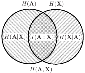
Figure 2: Venn diagram for classical information. $H({\bf A})$ is the entropy associated with a measurement of ${\bf A}$: it is the information needed to completely determine its outcome. $H({\bf X})$ is the same quantity for the observable ${\bf X}$. $H({\bf A},{\bf X})$ is the joint entropy of ${\bf A}$ and ${\bf X}$. $H({\bf A}|{\bf X})$ is the average uncertainty about ${\bf A}$ remaining after a measurement of ${\bf X}$. The information learned about ${\bf A}$ by measuring ${\bf X}$ is thus $I({\bf A}:{\bf X})=H({\bf A})-H({\bf A}|{\bf X})$. The equivalent definition $I({\bf A}:{\bf X})=H({\bf A})+H({\bf X})-H({\bf A},{\bf X})$ can also be understood from the diagram. These two definitions of the mutual information are equivalent Cover and Thomas (1991) when probabilities can be consistently assigned to the outcomes of all the possible measurements of ${\bf A}$ and ${\bf X}$ both separately and jointly: this is ensured when ${\bf A}$ and ${\bf X}$ commute. They need not coincide otherwise.

Of particular interest to us is the maximum amount of information about observable ${\bf A}$ of ${\mathcal{S}}$ that can be gained by measuring a fragment ${\mathcal{F}}$ of the environment. This is defined as

$$\hat{I}_{{\mathcal{F}}}({\bf A})=\max_{{\bf X}\in\mathcal{M}_{\mathcal{F}}}I({\bf A}:{\bf X})$$ (11)

where $\mathcal{M}_{\mathcal{F}}$ is the set of measurements acting on ${\mathcal{F}}$ only, i.e. the set of Hermitian operators that act trivially on ${\mathcal{H}}^{\overline{\mathcal{F}}}=\bigotimes_{{\mathcal{E}}_{k}\in\overline{\mathcal{F}}}{\mathcal{H}}^{{\mathcal{E}}_{k}}$. The “hat” above is to emphasize that it is the maximum amount of information.

In particular, the maximum amount of information about the system observable ${\bf A}$ that can be retrieved from the entire environment is denoted by $\hat{I}_{\mathcal{E}}({\bf A})$. This quantity plays a crucial role in our analysis as only when $\hat{I}_{\mathcal{E}}({\bf A})\approx H({\bf A})$ can we hope to “find out” about ${\bf A}$ by probing the environment: the amount of information in the environment, $\hat{I}_{\mathcal{E}}({\bf A})$, must be sufficiently large to compensate for the observer’s initial ignorance, $H({\bf A})$, about the value of ${\bf A}$.

IV.2 Redundancy of information in the environment

When $\hat{I}_{\mathcal{E}}({\bf A})\approx H({\bf A})$, the value of ${\bf A}$ can be found out indirectly by probing the environment. However, as noted in Section II, for many observers to arrive at a consensus about the value of an observable ${\bf A}$, there must be many copies of this information in ${\mathcal{E}}$. As a consequence, independent observers will be able to perform measurements on disjoint subsets of the environment, without the risk of invalidating each other’s observations.

Redundancy is therefore defined as the number of disjoint subsets of the environment containing almost all — all but a fraction $\delta$ — of the information about ${\bf A}$ present in the entire environment. Formally, let ${\mathcal{F}}_{1},{\mathcal{F}}_{2},\ldots,{\mathcal{F}}_{R}$ be $R$ disjoint fragments of the environment, ${\mathcal{F}}_{i}\cap{\mathcal{F}}_{j}=\emptyset$ for $i\neq j$. Then,

$$R_{\delta}({\bf A})$$ (12)

$$=\max_{\{{\mathcal{F}}_{j}\}}\left\{R:\hat{I}_{{\mathcal{F}}_{j}}({\bf A})\geq(1-\delta)\hat{I}_{\mathcal{E}}({\bf A}),\ \forall j=1,\ldots,R\right\}$$

where the maximization is carried over all partitions of $\{{\mathcal{E}}_{1},{\mathcal{E}}_{2},\ldots{\mathcal{E}}_{N}\}$ into disjoint subsets. Clearly, for any observable ${\bf A}$, $1\leq R_{\delta}({\bf A})\leq N$. Redundancy simply counts the number of copies of the imprint of ${\bf A}$ in ${\mathcal{E}}$, and hence the maximum number of observers that can independently find out about ${\bf A}$ from ${\mathcal{E}}$.

IV.3 Fragments of the environment and elementary subsystems

Before closing this section, we wish to emphasize the distinction we are making between fragments of ${\mathcal{E}}$ and elementary subsystems, and comment on the role they play in using environment as a witness. The elementary subsystems of ${\mathcal{E}}$ are defined through the natural tensor product structure of ${\mathcal{H}}^{\mathcal{E}}$. We assume this structure to be given and fixed. In the case of a photon environment for instance, an elementary subsystem could consist of a single photon. A fragment of ${\mathcal{E}}$ on the other hand is a collection of such elementary subsystems. For example, while no single photon can reveal the position of an object, a small collection of them, say 1000, may be enough to do so.

The optimization over partitions of the environment appearing at Eq. (12) is necessary to arrive at a proper mathematical definition of redundancy as there is no a priori preferred partition. This will allow us to derive very general consequences of redundancy, at the price of some technical (and perhaps also conceptual) complications. However, for the purposes of the emergence of a consensus among several observers — in essence an operational objective reality — this partition should reflect the distinct fragments of environment accessible to the different observers. While our results hold for any such partition of the environment into disjoint subsystems, Nature ultimately determines what part of ${\mathcal{E}}$ is available to each observer.

The entire environment as a witness approach — and more precisely the very concept of redundancy — capitalizes on the fact that the environment has a tensor product structure ${\mathcal{H}}^{\mathcal{E}}=\bigotimes_{{\mathcal{E}}_{k}}{\mathcal{H}}^{{\mathcal{E}}_{k}}$. This raises the obvious question “who decides what are the elementary subsystems of ${\mathcal{E}}$?” Our primary concern here is to provide a mechanism by which quantum systems can exhibit “objective existence”, the key symptom of the classical behavior. As we will demonstrate, this can be achieved given that the environment has a partition into subsystems, regardless of what these subsystems are. Hence, what really matters is that various observers monitor different fragments of the environment. As long as this requirement (which guarantees that the observables they measure commute) is fulfilled, their definition of subsystems of ${\mathcal{E}}$ need not coincide. Section V will present unavoidable consequences of this fact, without paying attention to the definition of the environmental subsystems. Thus, our most important conclusion, — that redundancy implies selection of preferred observables — is independent of any particular choice of a tensor product in the environment.

However, different tensor product structure of the environment can a priori yield different redundantly imprinted observables since redundancy itself makes reference to the tensor product structure. There is no definite answer to what defines an elementary environmental subsystem, but some considerations point towards “locality” as a judicious guideline. For instance, particles are conventionally defined by the symmetries of the fundamental Hamiltonians of Nature, that are local. When we choose the particles of the standard model as the elementary subsystems, we are naturally led to local couplings between ${\mathcal{S}}$ and ${\mathcal{E}}$. They will determine how the information is inscribed in ${\mathcal{E}}$. After all, “there is no information without representation”. Moreover, the information acquisition capacities of the observers are also ultimately limited by the fundamental Hamiltonians of Nature. The different observers occupy, and therefore monitor, different spatial regions. Therefore, the monitored fragments ${\mathcal{F}}_{i}$ entering in the definition of redundancy — as well as the elementary subsystems ${\mathcal{E}}_{k}$ composing them — should reflect these distinct spatial regions.

The fact that some division of the Universe into subsystems is needed has been pointed out before. Indeed, the measurement problem disappears when the Universe cannot be divided into subsystems Zurek (1993, 2003a); Schlosshauer (2004). Therefore, assuming that such division exists in the discussion of the information-theoretic aspects of the origin of the classical does not seem to be a very costly assumption.

V Consequences of redundancy

We now have all the necessary ingredients to study the consequences of the existence of redundant information about the system in the environment. Here, we derive several properties of the system’s redundantly imprinted observables, as well as properties of the environmental observables revealing this information. While each of these results is interesting in its own right, our ultimate goal is to combine them and to show that the redundancy singles out a preferred set of commuting observables, the already familiar pointer observables. Throughout this section, we assume the existence of a perfect and redundant record of the system observables ${\bf A},{\bf B},{\bf C},\ldots$ in the environment, i.e. $\hat{I}_{\mathcal{E}}({\bf A})=H({\bf A})$ and $R_{\delta=0}({\bf A})\gg 1$, and similarly for ${\bf B},{\bf C},\ldots$ The general case of imperfect imprints will be addressed in the next section. Let us begin by studying the consequences of the existence of a record about the value of ${\bf A}$ in the environment.

Lemma V.1

$\hat{I}_{\mathcal{F}}({\bf A})=H({\bf A})$, iff there exists an observable ${\bf X}^{\prime}\in\mathcal{M}_{\mathcal{F}}$ for which $H({\bf A}|{\bf X}^{\prime})=0$ and $H({\bf X}^{\prime}|{\bf A})=0$. The measurement of ${\bf X}^{\prime}$ on a fragment of the environment reveals all the information of the system observable ${\bf A}$, and vice versa.

Proof When observable ${\bf A}$ is completely encoded in a fragment of the environment, $\hat{I}_{\mathcal{F}}({\bf A})=H({\bf A})$, there exists ${\bf X}\in\mathcal{M}_{\mathcal{F}}$ for which $I({\bf A}:{\bf X})=H({\bf A})$, which implies $H({\bf A}|{\bf X})=0$. As noted in Section IV.1, the mutual information between ${\bf A}$ and ${\bf X}$ is symmetric when these observables act on distinct systems, i.e. ${\mathcal{S}}$ and ${\mathcal{F}}$. Therefore, measuring ${\bf A}$ directly on the system provides an amount of information $I({\bf A}:{\bf X})=H({\bf A})$ about the value of ${\bf X}$, thereby decreasing its entropy to $H({\bf X}|{\bf A})=H({\bf X})-H({\bf A})$. In general, this is not all the information about ${\bf X}$, as $H({\bf X})$ may be larger than $H({\bf A})$: ${\bf X}$ reveals all of the information about ${\bf A}$ but the reverse is in general not true. However, by picking a suitable coarse graining ${\bf X}^{\prime}$ of ${\bf X}$, it is always possible to establish the duality $H({\bf A}|{\bf X}^{\prime})=0$ and $H({\bf X}^{\prime}|{\bf A})=0$.

This can be seen quite simply. The equality $H({\bf A}|{\bf X})=0$ implies that given $X_{j}$, $A_{i}$ is determined: each measurement outcome of ${\bf X}$ points to a unique measurement outcome of ${\bf A}$. This defines a map $f:X_{j}\rightarrow A_{i}$. Such map may not be one-to-one, so the conditional probability $p(X_{j}|A_{i})$ of $X_{j}$ given $A_{i}$ is not necessarily deterministic. However, we can construct the coarse grained projectors

$$X_{i}^{\prime}=\sum_{j:f(X_{j})=A_{i}}X_{j}$$ (13)

by regrouping the $X_{j}$ in the pre-image of $A_{i}$. The outcome of the associated measurements ${\bf X}^{\prime}$ are therefore in one-to-one correspondence to the outcomes of ${\bf A}$, yielding the stated duality. The converse is trivial with $X=X^{\prime}$.  

An important corollary can be derived from Lemma V.1 and the following observation: when the outcome of a projective measurement on a system is deterministic, the act of measuring does not modify the state of the system.

Corollary V.1

Measurements of ${\bf A}$ and ${\bf X}^{\prime}$ have exactly the same effect on the joint state of the system and the environment:

$$X_{j}^{\prime}\rho^{{\mathcal{S}}{\mathcal{E}}}X_{j}^{\prime}=A_{j}X_{j}^{\prime}\rho^{{\mathcal{S}}{\mathcal{E}}}X_{j}^{\prime}A_{j}=A_{j}\rho^{{\mathcal{S}}{\mathcal{E}}}A_{j},$$ (14)

which implies $\rho^{{\mathcal{S}}{\mathcal{E}}}_{|\tilde{X}_{j}}=\rho^{{\mathcal{S}}{\mathcal{E}}}_{|A_{j}}$.

The contents of Lemma V.1 and Corollary V.1 formalize our intuitive understanding of the existence of a perfect record of the information about ${\bf A}$ in ${\mathcal{E}}$: it allows perfect emulation of the direct measurement ${\bf A}$ by the indirect measurement ${\bf X}^{\prime}$. This emulation is not only perfect from the point of view of its information yield, it also has the same physical effect on the state of ${\mathcal{S}}{\mathcal{E}}$. This can be regarded as an illustration of the fact that “information is physical” Landauer (1991): whenever the same information can be retrieved by two different means, the disturbance on the quantum state can be identical. Here, the measurement of ${\bf X}$ can in principle yield more information than the direct measurement ${\bf A}$ itself, e.g. ${\bf A}$ may be a very coarse grained observable. This is why it is in general necessary to coarse grain ${\bf X}$ in order to obtain equivalent information, and therefore the same physical effect.

Lemma V.2

When $\hat{I}_{\mathcal{F}}({\bf A})=H({\bf A})$, the observable ${\bf A}$ commutes with the reduced density matrix of the system, $[\rho^{\mathcal{S}},{\bf A}]=0$.

Proof Following Lemma V.1 and Corollary V.1, there exists ${\bf X}^{\prime}\in\mathcal{{\mathcal{E}}}$ for which $X_{j}^{\prime}\rho^{{\mathcal{S}}{\mathcal{E}}}X_{j}^{\prime}=A_{j}\rho^{{\mathcal{S}}{\mathcal{E}}}A_{j}$. The reduced state of the system can be therefore written as

$$\rho^{\mathcal{S}} = \mathrm{Tr}_{\mathcal{E}}\left\{\rho^{{\mathcal{S}}{\mathcal{E}}}\right\}$$ (15)

$$= \sum_{j}\mathrm{Tr}_{\mathcal{E}}\left\{X_{j}^{\prime}\rho^{{\mathcal{S}}{\mathcal{E}}}X_{j}^{\prime}\right\}$$ (16)

$$= \sum_{j}\mathrm{Tr}_{\mathcal{E}}\left\{A_{j}\rho^{{\mathcal{S}}{\mathcal{E}}}A_{j}\right\}=\sum_{j}A_{j}\rho^{{\mathcal{S}}}A_{j},$$ (17)

so $\rho^{\mathcal{S}}$ is block diagonal in the eigensubspaces of ${\bf A}$.  

The relation between decoherence and the existence of an environmental record has been pointed out and investigated in the past Zurek (1981, 1982, 1983, 1993, 2000); Gell-Mann and Hartle (1997); Zurek (1998); Halliwell (1999). The above lemma confirms that whenever the environment acquires a single copy of the information about ${\bf A}$, the state of ${\mathcal{S}}$ decoheres with respect to the spectral projectors $A_{i}$ of ${\bf A}$. This decoherence-induced diagonalization of the reduced state has additional important implications when the information about the system is encoded redundantly in the environment.

Corollary V.2

Let ${\bf A}$ be a system observable redundantly imprinted in ${\mathcal{E}}$, and let ${\bf X}^{\prime}$ be the coarse grained observable of the fragment ${\mathcal{F}}$ of the environment that contains all the information about ${\bf A}$ (as constructed in Lemma V.1). Then the reduced state $\rho^{{\mathcal{S}}{\mathcal{F}}}$ commutes with both ${\bf A}$ and ${\bf X}^{\prime}$: the correlations between these observables are classical.

Proof By assumption ${\bf A}$ is redundantly imprinted in ${\mathcal{E}}$. Thus, its value can be inferred by independent measurements, say ${\bf X}$ and ${\bf Y}$, acting on two distinct fragments of the environment, ${\mathcal{F}}$ and $\overline{\mathcal{F}}={\mathcal{E}}-{\mathcal{F}}$ respectively. Following Lemma V.1, we can construct a coarse grained observable ${\bf X}^{\prime}$ which retains essential correlations to ${\bf A}$ and with the property that $H({\bf X}^{\prime}|{\bf A})=0$ — a measurement of ${\bf A}$ on ${\mathcal{S}}$ reveals all the information about ${\bf X}^{\prime}$. As a consequence, the measurement ${\bf Y}$ on $\overline{\mathcal{F}}$ that reveals all the information about ${\bf A}$ must also reveals all the information about ${\bf X}^{\prime}$. Hence, Corollary V.2 follows from Lemma V.2.  

We will now characterize the class of system observables that can be redundantly imprinted in the environment. When ${\bf A}$ and ${\bf B}$ are redundantly imprinted in ${\mathcal{E}}$ and redundancy is sufficiently high, their value can be inferred from disjoint fragments of the environment. This implies the following relation between any redundantly imprinted observables.

Lemma V.3

Let ${\mathcal{F}}$ be a fragment of the environment containing a copy of the information about ${\bf A}$. When the rest of the environment $\overline{\mathcal{F}}$ contains a copy of the information about ${\bf B}$, then ${\bf A}$ and ${\bf B}$ necessarily commute on the support of $\rho^{\mathcal{S}}$.

Proof The assumptions of Lemma V.3 imply the existence of two environmental observables ${\bf X}$ and ${\bf Y}$ acting on disjoint fragments of the environment ${\mathcal{F}}$ and $\overline{\mathcal{F}}$ for which $H({\bf A}|{\bf X})=0$ and $H({\bf B}|{\bf Y})=0$. Following the procedure of Lemma V.1, we can coarse grain these two observables into ${\bf X}^{\prime}$ and ${\bf Y}^{\prime}$ that are in one-to-one correspondence with ${\bf A}$ and ${\bf B}$ respectively. The observables ${\bf X}^{\prime}$ and ${\bf Y}^{\prime}$ obviously commute with each other as they act on disjoint fragments of ${\mathcal{E}}$, and also commute with the system observables ${\bf A}$ and ${\bf B}$. Then, by Corollary V.1, we have

$$A_{i}B_{j}\rho^{{\mathcal{S}}{\mathcal{E}}}B_{j}A_{i} = A_{i}Y_{j}^{\prime}\rho^{{\mathcal{S}}{\mathcal{E}}}Y_{j}^{\prime}A_{i}=Y_{j}^{\prime}A_{i}\rho^{{\mathcal{S}}{\mathcal{E}}}A_{i}Y_{j}^{\prime}$$

$$= Y_{j}^{\prime}X_{i}^{\prime}\rho^{{\mathcal{S}}{\mathcal{E}}}X_{i}^{\prime}Y_{j}^{\prime}=X_{i}^{\prime}Y_{j}^{\prime}\rho^{{\mathcal{S}}{\mathcal{E}}}Y_{j}^{\prime}X_{i}^{\prime}$$

$$= X_{i}^{\prime}B_{j}\rho^{{\mathcal{S}}{\mathcal{E}}}B_{j}X_{i}^{\prime}=B_{j}X_{i}^{\prime}\rho^{{\mathcal{S}}{\mathcal{E}}}X_{i}^{\prime}B_{j}$$

$$= B_{j}A_{i}\rho^{{\mathcal{S}}{\mathcal{E}}}A_{i}B_{j},$$

proving the lemma.  

The above Lemma states that it is impossible to acquire perfect information about two non-commuting observables by measuring two disjoint fragments of ${\mathcal{E}}$ simultaneously. This is reminiscent of Heisenberg indeterminacy principle. However, in spite of this similarity, these two results differ in the precise setting in which they hold. Heisenberg principle asserts that it is impossible to know simultaneously the values of two non-commuting observables of an otherwise isolated system. In our Lemma, the system is already correlated with its environment, and the observer is trying to find out about the value of two observables using these correlations. In other words, Heisenberg indeterminacy concerns information about the system before it interacted with ${\mathcal{E}}$, while Lemma V.3 focuses on the information about ${\mathcal{S}}$ that is present in ${\mathcal{E}}$ after their interaction.

This difference illustrates the nature of our operational approach: we are describing the physical properties of an open quantum system, hence we focus on information about its present state, not on what it was prior to the interaction with ${\mathcal{E}}$. Decoherence happens, so we are dealing with it.

We can derive a similar result for the commutation of environmental observables.

Lemma V.4

Let ${\mathcal{F}}$ be a fragment of the environment containing information about both ${\bf A}$ and ${\bf B}$, two commuting system observables. Then, there exist two observables ${\bf X}^{\prime}$ and ${\bf Y}^{\prime}\in\mathcal{M}_{\mathcal{F}}$ that commute on the support of $\rho^{{\mathcal{S}}{\mathcal{E}}}$ and reveal all the information about ${\bf A}$ and ${\bf B}$ respectively.

Proof The assumptions of Lemma V.4 imply the existence of ${\bf X}$ and ${\bf Y}\in\mathcal{M}_{\mathcal{F}}$ such that $I({\bf A}:{\bf X})=H({\bf A})$ and $I({\bf B}:{\bf Y})=H({\bf B})$. Following the procedure of Lemma V.1, ${\bf X}$ and ${\bf Y}$ can be coarse grained to ${\bf X}^{\prime}$ and ${\bf Y}^{\prime}$ while retaining all the essential correlations to ${\bf A}$ and ${\bf B}$. Since ${\bf A}$ and ${\bf B}$ commute, the proof of Lemma V.3 can be applied here, yielding the desired result.  

Given these properties of redundantly imprinted observables, we can now state a very important result, which essentially ensures the uniqueness of redundantly imprinted observables.

Theorem V.1

Let ${\bf B}$ and ${\bf C}$ be two system observables redundantly imprinted in the environment, and let ${\mathcal{F}}_{1},{\mathcal{F}}_{2},\ldots,{\mathcal{F}}_{R}$ be $R\geq 2$ disjoint fragments of ${\mathcal{E}}$, each containing a copy of the information about ${\bf B}$ and ${\bf C}$. Then, there exists a refined system observable ${\bf A}$ satisfying:

1. $\hat{I}_{\mathcal{E}}({\bf A})=H({\bf A})$,

2. $R_{0}({\bf A})\geq R$,

3. $H({\bf B}|{\bf A})=0$ and $H({\bf C}|{\bf A})=0$.

Proof The assumptions of the theorem imply the existence of ${\bf Y}^{{\mathcal{F}}_{n}}$ and ${\bf Z}^{{\mathcal{F}}_{n}}\in\mathcal{M}_{{\mathcal{F}}_{n}}$ for which $H({\bf B}|{\bf Y}^{{\mathcal{F}}_{n}})=0$ and $H({\bf C}|{\bf Z}^{{\mathcal{F}}_{n}})=0$ for all $n=1,\ldots,R$. By Lemma V.3, ${\bf B}$ and ${\bf C}$ must commute as they can be inferred from disjoint fragments of the environment. This fact, together with Lemma V.4, implies that there exists commuting coarse grained observables ${\bf Y}^{\prime{\mathcal{F}}_{n}}$ and ${\bf Z}^{\prime{\mathcal{F}}_{n}}\in\mathcal{M}_{{\mathcal{F}}_{n}}$ that reveal all of the information about ${\bf B}$ and ${\bf C}$ respectively. The observables ${\bf B}$ and ${\bf C}$ can be merged into a more refined observable ${\bf A}$ with spectral projectors given by the product of the spectral projectors of ${\bf B}$ and ${\bf C}$:

$$A_{ij}=B_{i}C_{j}.$$ (18)

As $B_{i}$ and $C_{j}$ commute, the operators $A_{ij}$ form a complete set of mutually orthogonal projectors. Similarly, the environment observables ${\bf Y}^{\prime{\mathcal{F}}_{n}}$ and ${\bf Z}^{\prime{\mathcal{F}}_{n}}$ can be merged into a more refined observable ${\bf X}^{{\mathcal{F}}_{n}}$ with spectral projectors $X^{{\mathcal{F}}_{n}}_{ij}=Y^{\prime{\mathcal{F}}_{n}}_{i}Z^{\prime{\mathcal{F}}_{n}}_{j}$. A measurement of ${\bf X}^{{\mathcal{F}}_{n}}$ on ${\mathcal{F}}_{n}$ reveals all the information about ${\bf A}$. Indeed, following Corollary V.1,

$$p(A_{i^{\prime}j^{\prime}}|X_{ij}^{{\mathcal{F}}_{n}})=\frac{\mathrm{Tr}\left\{A_{i^{\prime}j^{\prime}}X_{ij}^{{\mathcal{F}}_{n}}\rho^{{\mathcal{S}}{\mathcal{E}}}X_{ij}^{{\mathcal{F}}_{n}}A_{i^{\prime}j^{\prime}}\right\}}{\mathrm{Tr}\left\{X_{ij}^{{\mathcal{F}}_{n}}\rho^{{\mathcal{S}}{\mathcal{E}}}X_{ij}^{{\mathcal{F}}_{n}}\right\}}$$

$$\quad=\frac{\mathrm{Tr}\left\{B_{i^{\prime}}C_{j^{\prime}}Y^{\prime{\mathcal{F}}_{n}}_{i}Z^{\prime{\mathcal{F}}_{n}}_{j}\rho^{{\mathcal{S}}{\mathcal{E}}}Z^{\prime{\mathcal{F}}_{n}}_{j}Y^{\prime{\mathcal{F}}_{n}}_{i}C_{j^{\prime}}B_{i^{\prime}}\right\}}{\mathrm{Tr}\left\{Y^{\prime{\mathcal{F}}_{n}}_{i}Z^{\prime{\mathcal{F}}_{n}}_{j}\rho^{{\mathcal{S}}{\mathcal{E}}}Z^{\prime{\mathcal{F}}_{n}}_{j}Y^{\prime{\mathcal{F}}_{n}}_{i}\right\}}$$

$$\quad=\delta_{ii^{\prime}}\delta_{jj^{\prime}}$$

which implies $H({\bf A}|{\bf X}^{{\mathcal{F}}_{n}})=0$. This automatically implies $\hat{I}_{{\mathcal{F}}_{n}}({\bf A})=H({\bf A})$ and, since the above holds for all $n=1,\ldots R$, we have $R_{0}({\bf A})\geq R$. Finally, note that $B_{i}=\sum_{j}A_{ij}$ and $C_{j}=\sum_{i}A_{ij}$; ${\bf B}$ and ${\bf C}$ are obtained by coarse graining ${\bf A}$. Therefore, a measurement of ${\bf A}$ reveals all the information about ${\bf B}$ and ${\bf C}$, hence completing the proof.  

The meaning of this Theorem is that whenever more than one observable can be redundantly inferred from a fixed set of disjoint fragments of ${\mathcal{E}}$, they necessarily correspond to some coarse grained version of a maximally refined redundantly imprinted observable ${\bf A}$. The modus tollens of this Theorem is also very enlightening. Given a decomposition of ${\mathcal{E}}$ into fragments and the associated maximally refined redundantly imprinted observable ${\bf A}$, the only observables ${\bf B}$ that can be completely and redundantly inferred from these fragments of ${\mathcal{E}}$ are those for which $I({\bf B}:{\bf A})=H({\bf B})$. The value of ${\bf B}$ must be entirely determined by a measurement of the maximally refined ${\bf A}$. This is obviously a sufficient condition: if a direct measurement of ${\bf A}$ reveals all the information about ${\bf B}$ and ${\bf A}$ is redundantly imprinted in ${\mathcal{E}}$, then so is ${\bf B}$. Theorem V.1 shows that this requirement is also necessary.

Note that the proof relies only on a redundancy greater than $2$ and on a fixed decomposition of ${\mathcal{E}}$ into disjoint fragments from which ${\bf B}$ and ${\bf C}$ are inferred. Relaxing this last assumption raises the possibility that different decompositions lead to incompatible maximally refined redundant observables. Figure 3 represents two decompositions of ${\mathcal{E}}$ into fragments for which the corresponding maximally refined redundantly imprinted observables could not be compared through the above theorem. In absence of further assumptions on the dynamics that is responsible for the creation of correlations between ${\mathcal{S}}$ and fragments of ${\mathcal{E}}$, this possibility can be ruled out when redundancy is high (see Theorem V.2 below). For most practical cases—especially when the subsystems of ${\mathcal{E}}$ interact with ${\mathcal{S}}$ according to commuting hamiltonians—such complication can be avoided as the maximally refined observable is often independent of the decomposition of ${\mathcal{E}}$ into fragments.

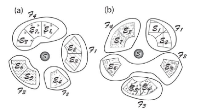
Figure 3: Suppose ${\bf B}$ and ${\bf C}$ are redundantly imprinted in the environment, but are associated respectively to decompositions (a) and (b), represented by different arrangements of the subsystems of ${\mathcal{E}}$ into fragments. Then, from Theorem V.1 one cannot yet conclude that there exists a maximally refined observable ${\bf A}$ from which both ${\bf B}$ and ${\bf C}$ can be inferred. This is because the two decompositions do not match. However, when the redundancy of ${\bf B}$ and ${\bf C}$ satisfies $R_{0}({\bf B})R_{0}({\bf C})>N$, then Theorem V.2 proves that the maximally refined observables obtained for each decomposition of ${\mathcal{E}}$ into fragments must commute (i.e. they are compatible).

Theorem V.2

Let ${\bf B}$ and ${\bf C}$ be two system observables both highly redundantly encoded in ${\mathcal{E}}$, such that $R_{0}({\bf B})\times R_{0}({\bf C})>N$. Then, $[{\bf B},{\bf C}]=0$ on the support of $\rho^{{\mathcal{S}}}$.

Proof By the assumptions of the Theorem, there exists a fragment ${\mathcal{F}}$ of size at most $N/R_{0}({\bf B})$ containing all information about ${\bf B}$. Since $R_{0}({\bf C})>N/R_{0}({\bf B})$, there exists a fragment ${\mathcal{F}}^{\prime}$ disjoint from ${\mathcal{F}}$, i.e. ${\mathcal{F}}\cap{\mathcal{F}}^{\prime}=\emptyset$, that contains all information about ${\bf C}$. By Lemma V.3 we have $[{\bf B},{\bf C}]=0$.  

It is intriguing to note that — in view of the above discussion — large redundancy implies $R>\sqrt{N}$. Theorems V.1 and V.2 prove our claim of Section II. Redundant spreading of information comes at the price of singling out a preferred set of commuting observables: those obtained by coarse graining maximally refined redundantly observables.

So far, we have not considered any dynamical evolution of the system and environment: we have focused on the correlations present at a fixed time without paying attention to how they arise. We studied consequences of regarding environment as a witness (and interrogating it about the state of the system), but we haven’t yet enquired about the dynamics that allowed the environment to acquire this information in the first place. Ultimately, it is the coupling Hamiltonian between ${\mathcal{S}}$ and ${\mathcal{E}}$ which establishes these correlations. The coupling is also responsible for the emergence of preferred system observables — the pointer observables — that are least affected by the openness of the system. Thus, as in the case of einselection of the pointer states, the connection between the emergence of an objective reality and the selection of preferred observables has to be ultimately traced to the dynamics responsible for the “environmental monitoring’ of ${\mathcal{S}}$ by ${\mathcal{E}}$ — i.e., through dynamical considerations. When the correlations between maximally refined observables and fragments of the environment persist in time, Lemma V.2 and Theorems V.1 & V.2 imply the following conclusion.

Corollary V.3

Highly redundantly imprinted observables are system’s pointer observables.

In other words, under the idealized assumption of perfect records we have demonstrated that only the already familiar pointer observables can leave a redundant and robust imprint on ${\mathcal{E}}$. Corollary V.3 can be understood as a consequence of the ability of the pointer states to persist while immersed in the environment. This resilience allows the information about the pointer observables to proliferate, very much in the spirit of the Darwinian “survival of the fittest”. This, along with other facts, will be illustrated on a dynamical model in the next section.

VI Quantum Darwinism: Dynamical emergence of objectivity

It should by now be clear that the presence of redundant information in the environment imposes severe physical constraints on the state of the system. Surprisingly, the derivation of these important facts required little physics — most of them followed from information-theoretic arguments, once again illustrating that information is physical. One could sum up our conclusions by noting that the environment can be a perfect witness — with multiple perfect records — but only for one set of commuting observables defined by the perfect maximally refined pointer observables. Such perfection will generally be only approximated in the real world. It is therefore important to investigate the situation where multiple, yet imperfect, copies arise through the dynamics. To this end we shall consider selective proliferation of information in a simple model that exhibits quantum Darwinism.

By focusing on the dynamics of ${\mathcal{S}}{\mathcal{E}}$ rather than on their state we will be able to extend our analysis. In particular, we will show that when the imprints of the objective observable are nearly perfect — i.e. $\hat{I}_{\mathcal{E}}({\bf A})\geq(1-\vartheta)H({\bf A})$ and $R_{\delta}({\bf A})>1$ for $\vartheta\ll 1$ and $\delta\ll 1$ finite but small — the conclusions obtained earlier still hold. Above all, along the lines of Theorem V.1, there exists a unique maximally refined observable whose information is the only one available in fragments of ${\mathcal{E}}$. Finally, we will be able to specify the optimal measurement to be performed on fragments of ${\mathcal{E}}$ to learn about the system. This is a considerable improvement over the result of the last section where, in the absence of any model Hamiltonian, we could only demonstrate the existence of such a measurement.

VI.1 Dynamics of Quantum Darwinism and decoherence

The model we consider is a generalization of the simple early model of decoherence put forward in Zurek (1982) and throughly investigated as a tractable, yet non-trivial, paradigm for decoherence: despite its simplicity, it captures the essence of einselection. Hence, our simple model serves as a special case that sets a conceptual framework for the study of more sophisticated models, such as a photon environment scattering on an object and carrying away potential visual data. As any specific model, it requires some fairly specific assumptions. We shall consider their role in the next section and discuss the extent to which relaxing some of these assumptions affects our conclusions.

A system ${\mathcal{S}}$ is coupled to an environment ${\mathcal{E}}=\{{\mathcal{E}}_{1},\ldots,{\mathcal{E}}_{N}\}$ through the Hamiltonian:

$${\bf H}^{{\mathcal{S}}{\mathcal{E}}}=\sum_{{\mathcal{E}}_{k}\in{\mathcal{E}}}{\bf A}\otimes{\bf Z}^{{\mathcal{E}}_{k}},$$ (19)

where ${\bf A}$ and ${\bf Z}^{{\mathcal{E}}_{k}}$ are operators acting on ${\mathcal{S}}$ and ${\mathcal{E}}_{k}$ respectively. The joint initial state of the system and the different environmental subsystems is assumed to be a pure product state:

$$|\Phi^{{\mathcal{S}}{\mathcal{E}}}(0)\rangle=|\phi^{\mathcal{S}}\rangle\otimes|\phi^{{\mathcal{E}}_{1}}\rangle\otimes|\phi^{{\mathcal{E}}_{2}}\rangle\otimes\ldots.$$ (20)

Hence, before the interaction, there is no correlation between the system and the environment, nor among the environmental subsystems.

A convenient way of writing $|\phi^{{\mathcal{S}}}\rangle$ in view of expressing the time evolution of the joint state of ${\mathcal{S}}{\mathcal{E}}$ is to decompose it in an eigenbasis $|i\rangle$ of ${\bf A}$ (${\bf A}|i\rangle=a_{i}|i\rangle$):

$$|\phi^{\mathcal{S}}\rangle=\sum_{i}\alpha_{i}|i\rangle.$$ (21)

Without loss of generality, we can assume that the vectors $|i\rangle$ with non-zero coefficients $\alpha_{i}$ in Eq. (21) are associated with distinct eigenvalues $a_{i}$ of ${\bf A}$. This can be done by choosing appropriate bases for the degenerate eigenspaces of ${\bf A}$. Thus, after an interaction time $t$ with the $N$ subsystems of the environment, the joint state of ${\mathcal{S}}{\mathcal{E}}$ evolves into:

$$|\Phi^{{\mathcal{S}}{\mathcal{E}}}(t)\rangle = \sum_{j}\alpha_{j}|j\rangle\bigotimes_{{\mathcal{E}}_{k}\in{\mathcal{E}}}e^{-ita_{j}{\bf Z}^{{\mathcal{E}}_{k}}}|\phi^{{\mathcal{E}}_{k}}\rangle$$ (22)

$$= \sum_{j}\alpha_{j}|j\rangle\bigotimes_{{\mathcal{E}}_{k}\in{\mathcal{E}}}|\phi_{j}^{{\mathcal{E}}_{k}}\rangle,$$ (23)

where we have defined $|\phi_{j}^{{\mathcal{E}}_{k}}\rangle=e^{-ita_{j}{\bf Z}^{{\mathcal{E}}_{k}}}|\phi^{{\mathcal{E}}_{k}}\rangle$.

In the following sections, we will analyze the correlations between the system ${\mathcal{S}}$ and the “observed” part of the environment ${\mathcal{F}}$. For example, in the case of a photon environment scattering on an object, ${\mathcal{F}}$ is the set of photons that hit the observer’s retina, while $\overline{\mathcal{F}}$ represents those photons that have scattered on ${\mathcal{S}}$ but that are not intercepted by the observer. Equation (23) allows us to compute the state of ${\mathcal{S}}$ and ${\mathcal{F}}$:

$$\rho^{{\mathcal{S}}{\mathcal{F}}}=\sum_{ij}\alpha_{i}\alpha_{j}^{*}|i\rangle\!\langle j|\otimes|\Phi_{i}^{\mathcal{F}}\rangle\!\langle\Phi_{j}^{\mathcal{F}}|\times\gamma^{\overline{\mathcal{F}}}_{ij},$$ (24)

where

$$|\Phi^{{\mathcal{F}}}_{j}\rangle=\bigotimes_{{\mathcal{E}}_{k}\in{\mathcal{F}}}e^{-ia_{j}{\bf Z}^{{\mathcal{E}}_{k}}t}|\phi^{{\mathcal{E}}_{k}}\rangle=\bigotimes_{{\mathcal{E}}_{k}\in{\mathcal{F}}}|\phi_{j}^{{\mathcal{E}}_{k}}\rangle\ ,$$ (25)

and $\gamma^{\overline{\mathcal{F}}}_{ij}=\prod_{{\mathcal{E}}_{k}\in\overline{\mathcal{F}}}\langle\phi^{{\mathcal{E}}_{k}}_{j}|\phi^{{\mathcal{E}}_{k}}_{i}\rangle=\langle\Phi_{j}^{\overline{\mathcal{F}}}|\Phi_{i}^{\overline{\mathcal{F}}}\rangle$. Similarly, the reduced state of the system at time $t$ reads:

$$\rho^{\mathcal{S}}=\sum_{ij}\alpha_{i}\alpha_{j}^{*}|i\rangle\!\langle j|\times\gamma^{\mathcal{E}}_{ij},$$ (26)

where $\gamma^{\mathcal{E}}_{ij}=\prod_{{\mathcal{E}}_{k}\in{\mathcal{E}}}\langle\phi^{{\mathcal{E}}_{k}}|e^{-it(a_{i}-a_{j}){\bf Z}^{{\mathcal{E}}_{k}}}|\phi^{{\mathcal{E}}_{k}}\rangle$. Above, the $\gamma$’s are called the decoherence factors.

Except in carefully controlled experiments — where the system can be very well isolated from its environment — the number of environmental subsystems interacting with ${\mathcal{S}}$ is huge. In this case, the $\gamma_{ij}^{\mathcal{E}}$’s will be typically very small for $i\neq j$. Each environmental subsystem contributes a factor $\langle\phi^{{\mathcal{E}}_{k}}|e^{-i(a_{i}-a_{j}){\bf Z}^{{\mathcal{E}}_{k}}t}|\phi^{{\mathcal{E}}_{k}}\rangle$ to $\gamma_{ij}^{\mathcal{E}}$, so unless $|\phi^{{\mathcal{E}}_{k}}\rangle$ is an eigenstate of ${\bf Z}^{{\mathcal{E}}_{k}}$ — in which case ${\mathcal{E}}_{k}$ is effectively decoupled from the system — this strictly decreases the decoherence factor. Hence, $\gamma_{ij}^{\mathcal{E}}$ goes to $\delta_{ij}$ as $N$ increases. To be more specific, when the initial states of the environmental subsystems are distributed uniformly at random, the decrease of $\gamma^{\mathcal{E}}_{ij}$ is exponential with $N$ and typically Gaussian with time Zurek et al. (2003).

This reasoning also applies to the decoherence factors $\gamma^{\overline{\mathcal{F}}}_{ij}$: they tend to zero for $i\neq j$ as the number of unobserved environmental subsystems increases. Even though a considerable number of the environmental subsystems can be intercepted by the observer, an even larger fraction will usually escape his monitoring. Thus, the $\gamma_{ij}^{\overline{\mathcal{F}}}$’s will also typically be very small for $i\neq j$.

We have numerically studied a version of this model (the case of two dimensional system and environmental subsystems) in Ollivier et al. (2004). Our results indicate that for sufficiently large environment, several system observables can become nearly perfectly imprinted in the environment (see Fig. 1a of Ollivier et al. (2004)). However, the results also clearly show that only those observables very “close” to the pointer observable can leave a redundant imprint in the environment (see Fig. 1b of Ollivier et al. (2004)). The information about the other system observables can only be accessed by measuring the entire environment: their value cannot be learned from small fragments of ${\mathcal{E}}$. In what follows, we will derive these facts analytically.

VI.2 Decoherence: the focus on the system

In order to contrast the environment as a witness approach to classicality as well as to illustrate significance of the dynamics that leads to quantum Darwinism, we will now review some results that were obtained using more conventional approaches. Thus, we will abandon for a moment the study of correlations between ${\mathcal{S}}$ and parts of the environment to focus uniquely on the state of the system, as it is done in the the standard studies of decoherence Giulini et al. (1996); Paz and Zurek (2001).

We see from Eq. (26) that the off-diagonal terms of the system’s density matrix tend to be very small when expressed in the $|i\rangle$ basis. It is therefore natural to expect that these are the quasi-classical states of the system: the coupling to the environment suppresses quantum superpositions of the states $|i\rangle$. Of course, the exact instantaneous diagonal basis of $\rho^{\mathcal{S}}$ might differ from $|i\rangle$, especially when the coefficients $\alpha_{j}$ of the system’s initial state Eq. (21) are almost equal. Hence, for someone focused on the instantaneous state of the system, it may not be clear why the basis $|i\rangle$ deserves any special attention in spite of the existence of small — yet non-zero — off-diagonal elements for $\rho^{\mathcal{S}}$. However, a simple analysis shows that the basis $|i\rangle$ is the only basis for which all off-diagonal terms tend to zero independently of the initial state of the system, and, thus, retain correlations with the rest of the Universe. This ability to retain correlations is behind the predictability of the pointer states — it is in fact their defining feature (see Zurek (1981, 1982) for the initial formulation, and Zurek (2003a, 2004); Schlosshauer (2004) for a recent re-assessment).

Persistence of correlations implies continued existence of the states Zurek (1998, 2003a). Independence of the pointer states from the initial state of the system is obviously a very important property of the to-be-classical states: the quasi-classical domain must be independent of the initial state of the system — e.g., the set of the pointer states of the apparatus should not depend on the state of the measured quantum system. When the system is initially prepared in one of the states $|i\rangle$, it will not be affected by the interaction with the environment: pointer states are stable. In more general cases (more complicated interactions, etc.), the above simple analysis cannot be carried out, and one usually relies on the predictability sieve Zurek (1993); Zurek et al. (1993); Giulini et al. (1996); Paz and Zurek (2001) to find the pointer basis. Predictability sieve seeks most predictable initial states — states that produce the smallest amount of entropy over time while subject to interaction with the environment.

VI.3 Perfect correlations

We now return to the study of the correlations between ${\mathcal{S}}$ and fragments of the environment. Our goal is to characterize what kind and how information is stored in the environment when it is redundant. To be more precise, we will analyze the structure of information in a fragment ${\mathcal{F}}$ of ${\mathcal{E}}$ under the assumption that the rest of the environment, i.e. $\overline{\mathcal{F}}={\mathcal{E}}-{\mathcal{F}}$, contains at least one additional copy of this information. Our demand that both ${\mathcal{F}}$ and $\overline{\mathcal{F}}$ contain a copy of the information ensures a minimum redundancy of $R\geq 2$ which — although insufficient to ensure the emergence of a consensus about the properties of ${\mathcal{S}}$ among many observers — is enough to re-derive directly most of the results established in Section V. In addition, we will be able to specify optimal measurement strategies on ${\mathcal{F}}$, the fragment of ${\mathcal{E}}$ accessible to the observer, for inferring any kind of information about ${\mathcal{S}}$.

To build our intuition, it is enlightening to first consider the limiting case $\gamma^{\overline{\mathcal{F}}}_{ij}=\gamma^{\mathcal{F}}_{ij}=\delta_{ij}$, where $\gamma_{ij}^{\mathcal{F}}=\langle\Phi_{i}^{\mathcal{F}}|\Phi_{j}^{\mathcal{F}}\rangle$. We return to the general case in Section VI.4. Following the general argument of Section VI.1, perfect correlation will be recovered when the environment is infinite. In our analysis, this condition reflects the physical assumption that both the observed and the unobserved fragments of ${\mathcal{E}}$ are very large. It is also possible to obtain perfect correlations in much smaller systems when the dynamics is fine-tuned so that the resulting state is GHZ-like. In either case, the density matrix of ${\mathcal{S}}$ and ${\mathcal{F}}$ reads

$$\sigma^{{\mathcal{S}}{\mathcal{F}}}=\sum_{i}|\alpha_{i}|^{2}|i\rangle\!\langle i|\otimes|\Psi^{{\mathcal{F}}}_{i}\rangle\!\langle\Psi^{{\mathcal{F}}}_{i}|$$ (27)

where the $|\Psi^{{\mathcal{F}}}_{i}\rangle$’s are mutually orthogonal. Note that $\rho$ and the $|\Phi^{\mathcal{F}}_{i}\rangle$’s of Eqs. (24-25) have been replaced respectively by ‘$\sigma$ and $|\Psi^{\mathcal{F}}_{i}\rangle$’s to emphasize $\gamma^{\mathcal{F}}_{ij}=\delta_{ij}$.

Consider the observable ${\bf X}\in\mathcal{M}_{\mathcal{F}}$ that perfectly distinguishes between the orthogonal states $|\Psi^{\mathcal{F}}_{i}\rangle$:

$${\bf X}=\sum_{i}x_{i}|\Psi^{\mathcal{F}}_{i}\rangle\!\langle\Psi^{\mathcal{F}}_{i}|=\sum_{i}x_{i}X_{i}.$$ (28)

Following Eq. (5), the state of the system after a measurement of ${\bf X}$ on ${\mathcal{F}}$ with outcome $X_{j}$ is

$$\sigma^{\mathcal{S}}_{|X_{j}}=\mathrm{Tr}_{\mathcal{F}}\{\sigma^{{\mathcal{S}}{\mathcal{F}}}_{|X_{j}}\}=\frac{\mathrm{Tr}_{\mathcal{F}}\{X_{j}\sigma^{{\mathcal{S}}{\mathcal{F}}}X_{j}\}}{p(X_{j})}=|j\rangle\!\langle j|.$$ (29)

This is the same as the state of ${\mathcal{S}}$ after a direct measurement of ${\bf A}$ with outcome $A_{j}$, $\sigma^{{\mathcal{S}}}_{|X_{j}}=\sigma^{{\mathcal{S}}}_{|A_{j}}$. Thus, a subsequent measurement of ${\bf A}$ on the system yields outcome $A_{i}$ with certainty, so $H({\bf A}|{\bf X})=0$. The same conclusion can be reached for a measurement acting on $\overline{\mathcal{F}}$: thus, ${\bf A}$ is encoded redundantly in ${\mathcal{E}}$ (there are at least two copies). As a consequence, all the results of Section V trivially hold (with exception of Theorem V.2). It is however instructive to derive them directly for our specific model, without appealing to the general lemmas.

As seen from Eq. (29), the indirect measurement ${\bf X}$ perfectly emulates the direct measurement ${\bf A}$ on the system. Consequently, all the information about the observable ${\bf A}$ can be extracted by the measurement ${\bf X}$ on the environment. In addition, we clearly see the “no-information / no-disturbance” principle at work: once the outcome of ${\bf X}$ is known, measuring ${\bf A}$ directly does not disturb the state of the system any further, as the measurement of ${\bf X}$ “projects” the system in an eigenstate of ${\bf A}$ (see Corollary V.1). Averaging over the measurement outcomes of ${\bf X}$ yields the reduced density matrix of ${\mathcal{S}}$, which is a mixture of the eigenstates of ${\bf A}$, so $[\rho^{\mathcal{S}},{\bf A}]=0$ as specified by Lemma V.2.

Specifying the Hamiltonian responsible for the correlations between ${\mathcal{S}}$ and its environment allows one to go beyond the purely information-theoretic analysis of Section V. Given the explicit form of the density matrix $\sigma^{{\mathcal{S}}{\mathcal{F}}}$, we can address more interesting questions such as: what is the optimal measurement ${\bf Y}$ on ${\mathcal{F}}$ that yields the largest amount of information about a given system observable ${\bf B}$? In fact, it turns out that ${\bf X}$ is the optimal measurement on ${\mathcal{F}}$ to find out the value of any system observable ${\bf B}$. Regardless of what we wish to learn about the system, the optimal strategy consists in measuring ${\bf X}$ on ${\mathcal{F}}$:

$$I({\bf B}:{\bf X})\geq I({\bf B}:{\bf Y})$$ (30)

for all ${\bf B}\in\mathcal{M}_{\mathcal{S}}$ and ${\bf Y}\in\mathcal{M}_{\mathcal{F}}$. Similarly, when a non-optimal measurement ${\bf Y}$ is carried on ${\mathcal{F}}$, it is always primarily correlated with the pointer observable ${\bf A}$. In other words, when a measurement ${\bf Y}$ is carried on a fragment of the environment, it always reveals more information about the pointer observable ${\bf A}$ than any other system observable:

$$I({\bf A}:{\bf Y})\geq I({\bf B}:{\bf Y})$$ (31)

for all ${\bf B}\in\mathcal{M}_{\mathcal{S}}$ and ${\bf Y}\in\mathcal{M}_{\mathcal{F}}$.

Let us prove these two very important assertions. First, note that following Eqs. (8,10), the mutual information between any system observable ${\bf B}$ and environmental observable ${\bf Y}$ takes the following form:

$$I({\bf B}:{\bf Y}) = H({\bf B})-H({\bf B}|{\bf Y})$$ (32)

$$= H({\bf Y})-H({\bf Y}|{\bf B}).$$ (33)

When ${\bf B}$ is a fixed system observable, maximizing $I({\bf B}:{\bf Y})$ amounts to minimizing $H({\bf B}|{\bf Y})$. To do this, consider the conditional state $\sigma^{{\mathcal{S}}}_{|Y_{i}}$ of the system given a measurement outcome $Y_{i}$ on ${\mathcal{F}}$. Simple algebraic manipulations can be used to show that

$$\sigma^{{\mathcal{S}}}_{|Y_{i}}=\frac{\mathrm{Tr}_{\mathcal{F}}\{Y_{i}\sigma^{{\mathcal{S}}{\mathcal{F}}}Y_{i}\}}{p(Y_{i})}=\sum_{j}p(X_{j}|Y_{i})\sigma^{\mathcal{S}}_{|X_{j}}.$$ (34)

We see that $\sigma^{{\mathcal{S}}}_{|Y_{i}}$ is a convex combination of the $\sigma^{{\mathcal{S}}}_{|X_{j}}$. (This is no coincidence: it follows from Corollary V.1, V.3, and the existence of information about ${\bf A}$, and hence about ${\bf X}$, in the rest of the environment $\overline{\mathcal{F}}$.) Hence, the inequality of Eq. (30) follows from the convexity of entropy, c.f. Proposition X.4. Similarly, when ${\bf Y}$ is a fixed measurement on ${\mathcal{F}}$, maximizing $I({\bf B}:{\bf Y})$ amounts to minimizing $H({\bf Y}|{\bf B})$. We can consider the state of ${\mathcal{F}}$ following a measurement of ${\bf B}$ on ${\mathcal{S}}$

$$\sigma^{{\mathcal{F}}}_{|B_{i}}=\frac{\mathrm{Tr}_{\mathcal{S}}\{B_{i}\sigma^{{\mathcal{S}}{\mathcal{F}}}b_{i}\}}{p(B_{i})}=\sum_{j}p(A_{j}|B_{i})\sigma^{\mathcal{F}}_{|A_{j}},$$ (35)

a convex combination of the states of ${\mathcal{F}}$ conditioned on a measurement of ${\bf A}$ on ${\mathcal{S}}$. Again, the inequality Eq. (31) follows from convexity of entropy, c.f. Proposition X.4.

By combining Eq. (30) with the fact that measuring ${\bf X}$ perfectly emulates the direct measurement ${\bf A}$ on ${\mathcal{S}}$, we get the following equality:

$$\hat{I}_{\mathcal{F}}({\bf B})=I({\bf B}:{\bf A}).$$ (36)

The information about ${\bf B}$ accessible from the fragment ${\mathcal{F}}$ is inherently limited by its correlation with the maximally refined observable ${\bf A}$. The only assumption required to arrive at this important equality is that correlations with both the observed and the unobserved parts of the environment impose $\gamma^{{\mathcal{F}}}_{ij}=\gamma^{\overline{\mathcal{F}}}_{ij}=\delta_{ij}$. This requirement is, according to Corollary V.2, equivalent to saying that both ${\mathcal{F}}$ and $\overline{\mathcal{F}}$ contain a perfect copy of the information about ${\bf A}$.

The consequences of Equation (36) can be better appreciated once we recognize that it allows to evaluate the redundancy for any system observable straightforwardly. When the value of ${\bf B}$ can be deduced from knowledge of the value of ${\bf A}$, then each fragment of ${\mathcal{E}}$ containing information about ${\bf A}$ will inevitably contain information about ${\bf B}$. Formally,

$$I({\bf B}:{\bf A})\geq(1-\delta)\hat{I}_{\mathcal{E}}({\bf B})\Rightarrow R_{\delta}({\bf B})\geq R_{\delta=0}({\bf A}).$$ (37)

On the other hand, when the value of ${\bf B}$ cannot be deduced from knowledge of ${\bf A}$, ${\bf B}$ cannot be redundant:

$$I({\bf B}:{\bf A})<(1-\delta)\hat{I}_{\mathcal{E}}({\bf B})\Rightarrow R_{\delta}({\bf B})=1.$$ (38)

This is because Eq. (36) holds as long as $\bar{\mathcal{F}}$ contains information about ${\bf A}$. To have $\hat{I}_{{\mathcal{F}}}({\bf B})\geq\hat{I}_{{\mathcal{E}}}({\bf B})$, forces to take $\bar{\mathcal{F}}$ small enough so that it does not contain much information about ${\bf A}$. By virtue of Eq. (30), $\bar{\mathcal{F}}$ also contains little information about ${\bf B}$, implying $R_{\delta}({\bf B})=1$.

Note that these results can also be derived with the help of the data processing inequality (see Proposition X.5). In effect, the update rule of Eq. (5) shows that the sequence of measurements ${\bf B}$, ${\bf A}$, ${\bf X}$, ${\bf Y}$ forms a Markov chain (${\bf B}$ and ${\bf Y}$ are arbitrary): the joint probability of the measurement results of ${\bf B}$, ${\bf A}$, ${\bf X}$, ${\bf Y}$ satisfies

$$p(Y_{i},X_{j},A_{k},B_{l})=p(Y_{i}|X_{j})p(X_{j}|A_{k})p(A_{k}|B_{l})p(B_{l}),$$ (39)

yielding Eqs. (30,31) directly. This alternative derivation provides a very clear interpretation of our previous result. Trying to gather information about ${\bf B}$ (instead of ${\bf A}$) with the indirect measurement ${\bf Y}$ (instead of ${\bf X}$) can be viewed as the addition of noise over the perfect communication channel that allows the transmission of information about ${\bf A}$ in the environment.

Equations (37-38) extend Theorem V.1 to imperfect redundant imprints (i.e. finite $\delta$). Only observables “close” to the maximally refined redundant observable ${\bf A}$ — where closeness is measured with the help of mutual information — can leave a redundant (even imperfect) imprint in their environment. Moreover, it confirms the behavior found in the numerical study presented in Ollivier et al. (2004).

VI.4 Imperfect correlations

The previous section analyzed the consequences of perfect correlations between ${\mathcal{S}}$ and ${\mathcal{F}}$ in terms of optimal measurement strategies. However, perfect correlations are rarely found in Nature. Even for our simple model, perfect correlations can be assumed only in an asymptotic limit, as $N$ tends toward infinity, or by a careful tuning of the interaction time and strength. Hence, it is important to understand what happens when the conditions are not perfect. Here, we show that nearly perfect correlations — $\gamma^{\mathcal{F}}$ and $\gamma^{\overline{\mathcal{F}}}$ sufficiently small — are enough to ensure the validity of the results established above, up to small correction terms.

The technique we use is inspired by perturbation theory. It relies on the construction of a “perfectly correlated” state $\sigma^{{\mathcal{S}}{\mathcal{F}}}$ of the form Eq. (27) which is “close” to the actual state $\rho^{{\mathcal{S}}{\mathcal{F}}}$ of Eq. (24) generated by the dynamics. Then, using various bounds on entropies, we will conclude that all the information-theoretic quantities extracted from the ideal $\sigma^{{\mathcal{S}}{\mathcal{F}}}$ are approximately equal to those extracted from the actual $\rho^{{\mathcal{S}}{\mathcal{F}}}$. We will also examine the regime of validity of this approximation.

Let us define

$$\sigma^{{\mathcal{S}}{\mathcal{F}}}=\sum_{i}|\alpha_{i}|^{2}|i\rangle\!\langle i|\otimes|\Psi^{\mathcal{F}}_{i}\rangle\!\langle\Psi^{\mathcal{F}}_{i}|,$$ (40)

where the $|\Psi^{\mathcal{F}}_{i}\rangle$’s are obtained by applying the Gram-Schmidt orthonormalisation procedure to the states $|\Phi^{\mathcal{F}}_{i}\rangle$’s (see the appendix for the details of this construction). With this definition, we will show that for any two observables ${\bf B}$ and ${\bf Y}$, when $\gamma^{\mathcal{F}}=\max_{ij}{|\gamma^{\mathcal{F}}_{ij}|}$ and $\gamma^{\overline{\mathcal{F}}}=\max_{ij}{|\gamma^{\overline{\mathcal{F}}}_{ij}|}$ are small,

$$I_{\rho}({\bf B}:{\bf Y})\approx I_{\sigma}({\bf B}:{\bf Y}).$$ (41)

Above, the subscripts $\rho$ and $\sigma$ refer to the state, either the actual $\rho^{{\mathcal{S}}{\mathcal{F}}}$ or the perfect $\sigma^{{\mathcal{S}}{\mathcal{F}}}$, used to derive the probabilities of the measurement outcomes, that in turn are used to quantify information (this shorthand notation will be used in the rest of this section). Therefore, when Eq. (41) holds, all the conclusions derived from the perfect correlation case remain approximately true.

Equation (41) is a consequence of simple inequalities that give an upper bound on the difference $|I_{\rho}({\bf B}:{\bf Y})-I_{\sigma}({\bf B},{\bf Y})|$. First, Cauchy-Schwartz inequality (Proposition X.1) gives $\mathrm{Tr}\,|\rho^{{\mathcal{S}}{\mathcal{F}}}-\sigma^{{\mathcal{S}}{\mathcal{F}}}|\leq\sqrt{d^{{\mathcal{S}}}}\|\rho^{{\mathcal{S}}{\mathcal{F}}}-\sigma^{{\mathcal{S}}{\mathcal{F}}}\|_{2}$. Second, by definition of the trace distance between two density matrices (Definition X.1), $\sum_{ij}|p_{\rho}(B_{i},Y_{j})-p_{\sigma}(B_{i},Y_{j})|\leq\mathrm{Tr}\,|\rho^{{\mathcal{S}}{\mathcal{F}}}-\sigma^{{\mathcal{S}}{\mathcal{F}}}|$. Finally, by combining these results with Lemma X.1 and Fanne’s inequality (Proposition X.3) applied separately to each of the three entropies involved in $I({\bf B},{\bf Y})=H({\bf B})+H({\bf Y})-H({\bf B},{\bf Y})$, we find

$$|I_{\rho}({\bf B}:{\bf Y})-I_{\sigma}({\bf B}:{\bf Y})|$$ (42)

$$\quad\leq-3f(\gamma^{\mathcal{F}},\gamma^{\overline{\mathcal{F}}})\log(f(\gamma^{\mathcal{F}},\gamma^{\overline{\mathcal{F}}})/d^{\mathcal{S}})$$

$$\qquad+O((\gamma^{\mathcal{F}})^{3/4}+\gamma^{\overline{\mathcal{F}}}),$$

with $f(\gamma^{\mathcal{F}},\gamma^{\overline{\mathcal{F}}})=\sqrt{d^{\mathcal{S}}\{2(d^{\mathcal{S}}-1)(\gamma^{\mathcal{F}})^{2}+(\gamma^{\overline{\mathcal{F}}})^{2}\}}$. Thus, this difference tends to zero when $\gamma^{\mathcal{F}}$ and $\gamma^{\overline{\mathcal{F}}}$ tend to zero.

To gain further insight into the regime of validity of Eq. (41), recall that $\gamma^{\mathcal{F}}$ and $\gamma^{\overline{\mathcal{F}}}$ typically decrease exponentially with the number of environmental subsystems that have effectively interacted with ${\mathcal{S}}$. Therefore, for equation Eq. (41) to hold within constant accuracy, it is sufficient that each fragment ${\mathcal{F}}$ and $\overline{\mathcal{F}}$ contains a number of subsystems ${\mathcal{E}}_{k}$ scaling as $\log d^{\mathcal{S}}$ (or as a polynomial in $\log d^{\mathcal{S}}$). As discussed at the end of Section III, $d^{\mathcal{S}}$ is the effective dimension of the probed degree of freedom of ${\mathcal{S}}$, i.e. the number of distinguishable outcomes of an hypothetical measurement ${\bf B}$. Clearly then, $\log d^{\mathcal{S}}$ is generally much smaller than the size of the environment. Therefore, the conclusions drawn from the perfect correlation study remain essentially unchanged: ${\bf A}$ is the observable of the system that leaves the strongest imprint in fragments of the environment; the optimal environmental measurement to learn about any system observable is the one that reveals information about ${\bf A}$; and finally failing to interrogate ${\mathcal{F}}$ about ${\bf A}$ has the same effect as introducing noise in the measurement results. These conclusions hold to within an accuracy of roughly $\log d^{\mathcal{S}}/N$, which is enough in most situations involving macroscopic systems.

VII Discussion: Open questions and connections

Environment as a witness as well as quantum Darwinism — the dynamics responsible for the redundant imprinting of certain states that leads to their objectivity — are based on the same dynamical paradigm that is used in the study of decoherence and einselection. The to-be-classical “object of interest” (the system ${\mathcal{S}}$ or the apparatus ${\cal A}$) is immersed in the environment. What is now different — and this is a dramatic departure from the usual view of what matters — is the focus. Instead of analyzing either the state of ${\mathcal{S}}$ per se, or even the fate of the correlations between ${\mathcal{S}}$ and ${{\mathcal{A}}}$, attention shifts to the information available to the observer in fragments of ${\mathcal{E}}$.

This shift of focus has been precipitated by the realization Zurek (1993, 1998, 2000) that observers only rarely (if ever) acquire information by direct interaction with “systems of interest”: rather, we use ${\mathcal{E}}$ as a communication channel. The message — the state of the object of interest — is imprinted on ${\mathcal{E}}$ in multiple copies. However, the no-cloning theorem implies that arbitrary unknown states cannot be “advertised” throughout the environment in this fashion. Hence, as one can expect (and as our analysis indeed shows), selection of a preferred observable is a prerequisite for this redundant imprinting.

The basic intuition — the implication of the information-theoretic redundancy of the record for the emergence of the classical — was noted already some time ago Zurek (1982, 1983, 2000). It was refined into a more precise measure of redundancy — into $R_{\delta}$ we employed here — only recently Ollivier et al. (2004). Using this $\delta$-redundancy we have demonstrated — either under very specific assumptions of Ollivier et al. (2004), or in a still rather specific, but somewhat more general setting of this paper — that the familiar pointer observables are easiest to find indirectly, from the records imprinted on the fragments of the environment.

The aim of this section is to examine assumptions that went into our discussion and, by doing so, to explore the range of validity of our conclusions. The results obtained in Section V did not require any assumption about the physical model, but only apply to the case of perfect correlations. Thus, the model studied in Section VI is a convenient focus of attention. To establish uniqueness of a set of commuting preferred observables that is easiest to infer from ${\mathcal{E}}$ we have assumed that:

1. The initial state is a pure product state.

2. The system has no self-Hamiltonian.

3. Every environmental subsystem couples to the same system observable.

4. The environment has no Hamiltonian.

To find out which of these assumptions can be relaxed, and the extent to which they are responsible for the conclusions we have reached will eventually require investigation of other, more realistic, or at least “differently oversimplified” models. For “standard” decoherence, a similarly idealized model was put forward over two decades ago, but the investigation of various related and unrelated models of decoherence and einselection is still an ongoing activity, often yielding new insights. The same can be expected of quantum Darwinism. Different models may also require different mathematical tools. One such investigation — using von Neumann entropy and the symmetric Equation (10) for mutual information — is currently under way Blume-Kohout and Zurek and points toward compatible conclusions. All we can offer here is a brief (and possibly premature) discussion of the role and importance of various assumptions, including these listed above.

Assumption 1 is probably the most unrealistic: in practice composite environments are rarely in a pure product state. Luckily, perfect purity per se is not essential to rely on the environment as a trustworthy witness. Having enough information about ${\mathcal{E}}$ will, however — and in contrast to decoherence and einselection — prove to be indispensable.

Indeed, it is often convenient to study decoherence assuming a very mixed state of the environment (i.e., thermal equilibrium or even a perfect mixture) when deriving master equations used to implement predictability sieve. Consequences of different initial mixtures of ${\mathcal{E}}$ are, generally, somewhat different time dependences, and minor changes in the structure of the master equation (which often becomes less Markovian and less tractable when the environment is further away from a convincing thermal state), but the key qualitative conclusions that characterize decoherence and einselection — the localized nature of the preferred states and the fact that relaxation can be much slower than decoherence — seem to be usually unaffected.

By contrast, the degree of ignorance about the fragments of the environment plays an essential role in the study of the environment as a witness. The reader may be surprised by this. After all, the results of Section V and VI were derived by an information-theoretic analysis of a rather general scenario, so — given the assumptions — conclusions should be independent of the initial state of ${\mathcal{E}}$. In particular, redundancy — when present — remains a highly selective criterion. However, and this is the crux of the matter, the starting point of our investigation — the assumption that fragments of the environment contain information about the system — depends strongly on the initial state of ${\mathcal{E}}$.

When the environment is initially mixed, it will “know less” about the system. The change of the state of the environment after it has interacted with the system provides the evidence about the state of ${\mathcal{S}}$. But when either all of ${\mathcal{E}}$ or some subsystems of it are totally mixed, they cannot be altered by the conditional dynamics that causes decoherence. And even partial mixing will make it more difficult for the environment to serve as a wittness. To see why, let the initial state of the environment be an arbitrary non-entangled state:

$$\rho^{\mathcal{E}}=\sum_{\ell}p_{\ell}\bigotimes_{{\mathcal{E}}_{k}}|\phi^{\ell{\mathcal{E}}_{k}}\rangle\!\langle\phi^{\ell{\mathcal{E}}_{k}}|.$$ (43)

In particular, it could be a product of mixed states $\rho^{\mathcal{E}}=\rho^{{\mathcal{E}}_{1}}\otimes\rho^{{\mathcal{E}}_{2}}\otimes\ldots\rho^{{\mathcal{E}}_{N}}$, such as the thermal state of non-interacting environmental subsystems. By linearity of the Schrödinger equation, the joint state of ${\mathcal{S}}$ and a fragment ${\mathcal{F}}$ of ${\mathcal{E}}$ after an interaction time $t$ will be

$$\rho^{{\mathcal{S}}{\mathcal{F}}}=\sum_{\ell}p_{\ell}\sum_{ij}\alpha_{i}\alpha_{j}^{*}|i\rangle\!\langle j|\bigotimes_{{\mathcal{E}}_{k}}|\phi_{i}^{\ell{\mathcal{E}}_{k}}\rangle\!\langle\phi_{j}^{\ell{\mathcal{E}}_{k}}|\times\gamma_{ij}^{\ell\overline{\mathcal{F}}}$$ (44)

where $|\phi_{i}^{\ell{\mathcal{E}}_{k}}\rangle$ and $\gamma_{ij}^{\ell\overline{\mathcal{F}}}$ are defined as in Section VI.1.

In the previous sections, we have studied the kinds of correlations that arise given any of the components $\bigotimes_{{\mathcal{E}}_{k}}|\phi^{\ell{\mathcal{E}}_{k}}\rangle$ of this mixture. It follows from the convexity of entropy (c.f. Proposition X.4) that the information contained in this mixture will be strictly less than the average information contained in the individual components of the mixture. As we have noted above, mixing the state of the environmental subsystems decreases their information storage capacity; when the state of the environment is perfectly mixed, it will simply be impossible to learn anything from it. Yet, the usual decoherence still leads to einselection — there will still be a pointer basis (defined e.g. through the predictability sieve).

When the initial state of ${\mathcal{E}}$ is not completely mixed, it is usually possible to extract from it some information about the system. In fact, given the assumption of redundancy, the qualitative conclusions of the previous section will still hold: the information about any system observable available in fragments of ${\mathcal{E}}$ is intrinsically limited by the information about it obtained through a direct measurement of the maximally refined redundantly imprinted observable ${\bf A}$; Eq. (36) becomes the inequality $\hat{I}_{\mathcal{F}}({\bf B})\leq I({\bf B}:{\bf A})$. Therefore, we again anticipate the conclusion that only observables “close” to ${\bf A}$ can get redundantly imprinted in ${\mathcal{E}}$.

Mixed initial states of ${\mathcal{E}}$ will decrease channel capacity of the environment. Moreover, modes of the environment that can be imprinted with information about different aspects of ${\mathcal{S}}$ will be in general mixed to a different degree. This may be reflected in the selective coarse-graining with which the observer perceives the system. This raises an interesting possibility: observables that are selected by the predictability sieve need not coincide with the (typically coarse - grained) observables that are easiest to find out about from ${\mathcal{E}}$. For example, this may happen when the modes that dominate decoherence (and hence einselection) are so mixed that they cannot serve as a useful communication channel, and the only modes that are sufficiently pure to be useful for this purpose monitor some other observable. An observer will then find out about that other coarse-grained observable, but with the resolution limited by indeterminacy: after all, pointer observable is still einselected by the environmental monitoring! Presence or absence of this effect is related to the assumption of the “typical environment fragment” we have noted in Ollivier et al. (2004). In other words, when the fragments of ${\mathcal{E}}$ that the observer can use to extract information about ${\mathcal{S}}$ contain or reveal data in a selective manner, environment acts as a witness with a selective memory (or a partial amnesia). Exactly how mixed can ${\mathcal{E}}$ be to be still useful as a witness is of course the key question. We leave it as a subject for further research.

When the initial state of the system is mixed, but the environment is sufficiently pure and large so that significant redundant imprinting can arise from their interaction, environment can become a useful and trustworthy witness, and our approach should go through essentially unimpeded. Similarly, preexisting correlation with ${\mathcal{E}}$ need not undermine our conclusions. In effect, it will typically mean that the environment was gathering evidence about the system in the past (although one can certainly imagine pathological preexisting correlations that get undone by the subsequent interaction).

To sum up, while the assumption of the initial product state has simplified our analysis, it can be relaxed to some extent without undermining our basic conclusions. What is non-negotiable is the demand that the final state allows one to discern evidence about $\mathcal{S}$ in the fragments of $\mathcal{E}$. One can already anticipate that this demand will also put a constraint on the entanglement between the fragments of ${\mathcal{E}}$, as we shall note in the discussion of the assumption 4 below.

Assumption 2 precludes non-trivial evolution of the system. Relaxing it has been studied in the context of decoherence and einselection, and — as we have done above — we shall gain insight into its role in quantum Darwinism by recounting the implications of evolution for einselection, and analyzing their significance for the role of the environment as a witness.

In the studies of einselection the relative strength of the self-Hamiltonian ${\bf H}^{\mathcal{S}}$ and the interaction Hamiltonian ${\bf H}^{{\mathcal{S}}{\mathcal{E}}}$ is an important ingredient that decides the course and effect of einselection. When the self-Hamiltonian is negligible or when ${\bf H}^{\mathcal{S}}$ and ${\bf H}^{{\mathcal{S}}{\mathcal{E}}}$ commute, the environment monitors static states of the system — pointer states selected solely by the interaction Zurek (1981, 1982). In a sense, environment contains a record of a very uneventful history — things stay the same forever.

When the effect of ${\bf H}^{\mathcal{S}}$ is no longer negligible, these histories become more interesting. One may enter, for example, the “partial Zeno effect” regime where the evolution of the state of the system induced by the self-Hamiltonian is impeded (but not completely suppressed) by the environmental monitoring mediated by ${\bf H}^{{\mathcal{S}}{\mathcal{E}}}$ (see, e.g., Giulini et al. (1996)). Models of such situations have been analyzed using rather different approach of quantum trajectories Carmichael (1993) that shares with quantum Darwinism the focus on the information gained indirectly from ${\mathcal{E}}$. There the environment is usually assumed to consist of photons, and the system is often a two-level “atom”. Pointer states still emerge and turn out to be the easiest states to infer from a fraction of such ${\mathcal{E}}$ Dalvit et al. (2001). The basis ambiguity may reappear only if the whole ${\mathcal{E}}$ could be captured. This ability to rely on a fraction of ${\mathcal{E}}$ allows for the possibility of consensus between multiple observers Dalvit et al. (2004).

As the coupling to the environment becomes weak the problem may become more tractable again, especially in two rather different limits. When the environment is slow, with the high-frequency cutoff that is small compared to the level spacing of the spectrum of ${\bf H}^{\mathcal{S}}$, einselection enters its quantum limit Paz and Zurek (1999). Energy eigenstates are imprinted on the environment more or less regardless of the specific form of the coupling. Histories are again becoming rather uneventful, although for reasons quite different from these we have mentioned above in the negligible ${\bf H}^{\mathcal{S}}$ case.

By contrast, when the environment is “broadband”, with all the frequencies from very low to very high present, and the system is (at least approximately) linear and coupled to ${\mathcal{E}}$ through its position, coherent states are the most predictable, and hence, pointer. Weak coupling does not preclude redundancy of the records. In this underdamped limit one can recover approximately reversible Liouvillian dynamics with localized states (i.e., approximately reversible classical trajectories that follow Newton’s laws emerge; see Paz and Zurek (2001); Zurek (2003a), and references therein). When the system is linear (e.g., harmonic oscillator) preferred pointer states turn out to be Gaussian Zurek (1993); Zurek et al. (1993), and one may anticipate that sequences of the most redundant “environmental records” will correlate with classical trajectories.

The quick summary of different possibilities above is meant to be suggestive rather than exhaustive, and is definitely not conclusive. What one would like to recover using environment as a witness is the notion of objective histories defined through sequences of time-ordered redundant records. Such objective histories could consist of sequences of approximate instantaneous pointer states. They were conjectured to exist in the limit of very efficient and frequent broad-band monitoring by the environment in Zurek (2003a). Histories deduced from redundant records would be objective, and may be only approximate. It will be interesting to investigate their relation to consistent histories Griffiths (1984); Gell-Mann and Hartle (1990); Omnès (1992); Omn99a ; Gri02a , especially when consistency is assured through the “strong decoherence” condition introduced in Gell-Mann and Hartle (1997) (see also Halliwell (1999)) that invokes existence of a perfect environmental record.

Assumption 3 assures that there is a preferred observable of ${\mathcal{S}}$ that is recorded by ${\mathcal{E}}$, and that it is singled out by the interaction Hamiltonian. This is a strong assumption, but often a reasonably realistic one: typical couplings between the systems (and, hence, between ${\mathcal{S}}$ and ${\mathcal{E}}$) tend to depend on the distance (i.e., relative position) between them. As a consequence — as was already pointed out in the context of einselection Zurek (1982, 1991) — pointer states tend to be localized in position.

One can of course imagine situations where this is not the case. For instance, there may be several physically distinct environments, each attempting to monitor a different observable of ${\mathcal{S}}$. One would expect that a dominant coupling would then impose its selection of the preferred observable, and the effect of the others would be perceived as noise.

This last remark leads to interesting questions about the correspondence between the approximate pointer observable that is selected by the predictability sieve as a result of the interaction of $\mathcal{S}$ with $\mathcal{E}$, and the states of the system that are easiest to infer for an observer who has access to a single subsystem of the environment. Clearly, in full generality this case is not covered by our idealized assumptions earlier in the paper. For example, Gaussian pointer states are often selected by the predictability sieve, and yet they are not orthogonal and form an overcomplete basis, so some of the steps we have used in our proofs may not go through. Nevertheless, one may expect that — as was the case with decoherence — results that are exact for perfect pointer states (that are left untouched by decoherence) are still approximately valid for approximate pointer states (that are least touched by decoherence). Thus, even when the environment fragments that are the most useful channel to the observer interested in ${\mathcal{E}}$ are not a typical sample of the environments responsible for decoherence, one may still guess that the states of ${\mathcal{S}}$ that can be inferred from them will represent an appropriately coarse-grained versions of the pointer states. Given the role Gaussian states play in the discussion of various models of decoherence, the extent to which Gaussian states coincide with the states that are easiest to infer is of obvious interest, and a likely area of future studies, but beyond the scope of this paper (see however Dalvit et al. (2005)). Along the same line of thought, when the environment fragments that are the most useful to the observer interested in $\mathcal{S}$ are not a typical sample of the environments responsible for decoherence, one may still guess that the states of $\mathcal{S}$ that can be inferred from them will represent an appropriately coarse-grained versions of the pointer states.

Given the role Gaussians play in discussion of various models of decoherence, the extent to which Gaussians that are most predictable coincide with the states that are easiest to infer is of obvious interest, and a likely area of future studies, but beyond the scope of this paper.

Assumption 4 assures that the environment does not evolve (and, therefore, does not complicate or even obliterate the record it has made of ${\mathcal{S}}$). More careful study of the consequences of relaxing this assumption can be found elsewhere Blume-Kohout and Zurek . Here we offer only a brief discussion of the basic possibilities.

One can distinguish three components of this requirement: fragments of the environment could evolve separately, they could interact with each other, or could interact with more distant “second order” environments.

Let us first note that — in models where pointer observable commutes with the system-environment interaction Hamiltonian (e.g. ${\bf H}^{{\mathcal{S}}{\mathcal{E}}}=\sum_{{\mathcal{E}}_{k}\in{\mathcal{E}}}{\bf A}\otimes{\bf Z}^{{\mathcal{E}}_{k}}$, Eq. (19)) self-Hamiltonians of the individual fragments of ${\mathcal{E}}$ obviously cannot change the fact that $[{\bf H}^{{\mathcal{S}}{\mathcal{E}}},{\bf A}]=0$, so the selection of the pointer basis is not affected by the dynamics of the environment. However, even in this simple case the presence of such self-Hamiltonians can influence the rate of acquisition of information by ${\mathcal{E}}$ and, hence, redundancy Blume-Kohout and Zurek . We also note that in more realistic cases when the system has a self-Hamiltonian that does not commute with ${\bf H}^{{\mathcal{S}}{\mathcal{E}}}$ the pointer observable is approximate, and even its choice can be influenced by how the rate of information acquisition by ${\mathcal{E}}$ compares with the dynamical timescales in ${\mathcal{S}}$.

The interaction between the subsystems of ${\mathcal{E}}$ may be a significant complication. It will typically lead to entanglement between the fragments of ${\mathcal{E}}$, and could make their individual states mixed. Thus, — as we have already pointed out in discussion of assumption 1 — even though the environment as a whole may still contain redundant imprint of the state of the system, the relevant global observables could become effectively inaccessible to the observers who can sample ${\mathcal{E}}$ only through local measurements on its fragments.

Last but not least, ${\mathcal{E}}$ could be immersed in its own environment ${\mathcal{E}}^{\prime}$. Effect of this second-order environment will depend on the nature of their interaction. It could of course erase the records of ${\mathcal{S}}$ in ${\mathcal{E}}$, but it is also conceivable that ${\mathcal{E}}^{\prime}$ could monitor the record-keeping observables of the fragments of ${\mathcal{E}}$, which would increase the redundancy Zurek (2003a).

These are very interesting complications, very much worthy of further study. We note, however, that human observers tend to rely on photons for the vast majority of data about “systems of interest”. And photons, in effect, satisfy our assumption 4. This seems to us to be no accident.

It is clear from the above discussion that quantum Darwinism requires stronger assumptions than decoherence. This is not surprising: it is easier to use any system (including the environment) as a disposal, to get rid of unwanted information, than as a communication channel. Furthermore, existence of the pointer states is a necessary but not a sufficient condition for their redundant imprinting on ${\mathcal{E}}$. Nevertheless, even though quantum Darwinism relies on stronger assumptions than einselection implemented e.g. through the predictability sieve, it is also clear from our discussion that these more restrictive assumptions are met in the real world often enough to employ environment as a reliable witness.

VIII Summary and Conclusion

Observers use environment as a witness. This has obvious and profound implications for the interpretation of quantum theory. Nevertheless, it is not our intent here to go beyond the comments we have made throughout and to delve into a more extensive discussion of the implications of quantum Darwinism for the interpretation of quantum theory. In part, this is because some of the interpretational issues have been noted elsewhere, on the occasion of discussions of the role of redundancy in the existential interpretation (see Zurek (1993, 1998, 2003a, 2003b), and references therein). The basic idea — that the classical domain can arise from within a quantum Universe, and that it consists of states that can be found out without being destroyed, and, hence, in that operational sense exist independently of the observer — is obviously very much assisted by employing environment as a witness.

Quantum Darwinism uses the same model of the information transfer that was introduced to study decoherence and einselection, but asks a different question: instead of focusing — as does decoherence — on how the information is lost from the system, it analyzes how the information is gained and stored in the environment. In decoherence, the role of the environment is limited to hiding the underlying quantumness (view especially emphasized in discussions of quantum computation). Einselection recognizes that this information loss is selective, and, thus, that the environment has a capacity to single out preferred pointer states that are best at surviving immersion in ${\mathcal{E}}$. Moreover, they are chosen in the process reminiscent of a measurement — ${\mathcal{E}}$ acts as an apparatus that (pre-)measures the pointer observable of the system of interest.

This much was known. In particular, the monitoring role of ${\mathcal{E}}$ was recognized early on Zurek (1981). Quantum Darwinism answers to the next logical question: since the environment interacts with the to-be-classical observable of the system of interest as would an apparatus, can it be used as an apparatus? To address it we have had to develop a measure of the objectivity of the records deposited in the environment. Redundancy (briefly considered Zurek (1983), see also Zurek (1982) in a similar context as a measure of amplification) was refined Ollivier et al. (2004) and used to prove that — given reasonable assumptions — there is a unique set of commuting observables that are easiest to find out from fragments of ${\mathcal{E}}$, and that these redundantly recorded observables are indeed the familiar pointer observables.

As a consequence, observers monitoring fragments of the environment will be able to reach compatible conclusions about the value of redundantly imprinted observables of the system, i.e. about the objective properties of the system. In this operational sense, quantum Darwinism provides a satisfying explanation for the emergence of the objective classical world we perceive from the underlying quantum substrate.

We have illustrated quantum Darwinism on a dynamical model that is easy to analyze from an information-theoretic perspective, and yet is inspired by a photon environment scattering on an object: all the environmental subsystems couple to the object with the same Hamiltonian and do not interact with each other. This model enabled us to push our analysis further, as we could explicitly determine the optimal environmental measurements to learn about the properties of the system. It also demonstrated that quantum Darwinism tolerates reasonable departures from the “ideal” assumptions used to derive our main results in Section V. In this respect, it corroborates recent studies Zurek (2003a); Ollivier et al. (2004) and earlier conjectures Zurek (1983, 2000) that noted the role of redundancy in assuring resilience of certain states — an essential feature of the classical domain. Hence, redundancy is a robust and selective criterion for determining objective properties of open quantum systems.

While redundantly imprinted observables are dynamically stable — as defined by einselection — the reverse is not necessarily true: quantum Darwinism requires stronger assumptions, especially regarding structure, size, and the initial state of ${\mathcal{E}}$. For example, a single photon can be enough to decohere an object in superposition of two distinct positions. However, it takes a macroscopic number of them to redundantly broadcast the position of this object throughout the environment. While the entropy production of the system — a signature of decoherence — rapidly saturates, redundancy can then continue to grow with time. This illustrates how the increase of the redundancy of the record in the environment captures the fact that the system is still continuously “under observation”, and that information about the pointer observable is getting amplified up to the macroscopic level. In this sense, quantum Darwinism can be motivated using Bohr’s original ideas Bohr (1928) about the role of amplification in the transition from quantum to classical.

IX Acknowledgments

We would like to thank Robin Blume-Kohout for extensive and enjoyable discussions. This research was supported in part by NSA and ARDA. H.O. receives financial support from ACI Sécurité Informatique, and D.P. from Canada’s NSERC and Québec’s NATEQ.

X Appendix

Definition X.1 (Trace distance)

The trace distance between two density operators $\rho$, $\sigma$ is defined by $D(\rho,\sigma)=\mathrm{Tr}\,|\rho-\sigma|$. When $\rho$ and $\sigma$ commute, the trace distance is equal to the $L_{1}$-distance between the classical probability distributions defined by their eigenvalues. Alternatively, the trace distance is equal to $2\max_{P}\mathrm{Tr}\,P(\rho-\sigma)$ where the maximum is taken over positive operators $P\leq I$

Definition X.2 (Euclidean distance)

The Euclidean distance between a pair of density operators $\rho$, $\sigma$ is defined by $\|\rho-\sigma\|_{2}=\sqrt{\mathrm{Tr}\left\{(\rho-\sigma)^{2}\right\}}$.

Proposition X.1 (Cauchy-Schwartz inequality)

$D(\rho,\sigma)\leq\sqrt{d}\|\rho-\sigma\|_{2}$.

Proposition X.2

Let $p_{i}=\mathrm{Tr}\{A_{i}\rho\}$ and $q_{i}=\mathrm{Tr}\{A_{i}\sigma\}$ be the probabilities of the outcomes of a measurement $\{A_{i}\}$ for states $\rho$ and $\sigma$ respectively. Then, $D(p,q)\leq D(\rho,\sigma)$.

Proposition X.3 (Fanne’s inequality)

Let $p_{i}$ and $q_{i}$ with $i=1,2,\ldots,d$ be two classical probability distributions such that $D(p,q)\leq 1/e$. Then $|H(p)-H(q)|\leq D(p,q)\log d+\eta(D(p,q))$, with $\eta(x)=-x\log x$.

Proposition X.4 (Convexity of entropy)

Let $P(X_{i}|Y_{j})$ be a set of conditional probability distribution for the random variable $X$, and $P(Y_{j})$ be the probability distribution for the random variable $Y$. Then

$$\sum_{j}\left[P(Y_{j})\left(-\sum_{i}P(X_{i}|Y_{j})\ln P(X_{i}|Y_{j})\right)\right]$$

$$\quad\leq-\sum_{i}P(X_{i})\ln P(X_{i})$$ (45)

where $P(X_{i})=\sum_{j}P(X_{i}|Y_{j})P(Y_{j})$.

Proposition X.5 (Data processing inequality)

Suppose $X\rightarrow Y\rightarrow Z$ is a Markov chain, then $H(X)\geq I(X:Y)\geq I(X:Z)$.

Lemma X.1

For any matrix $\rho=\sum_{ij}\alpha_{i}\alpha_{j}^{*}|i\rangle\!\langle j|\otimes|\Phi^{\mathcal{F}}_{i}\rangle\!\langle\Phi^{\mathcal{F}}_{j}|\gamma_{ij}^{\overline{\mathcal{F}}}$, with $\alpha_{i}\neq 0$, and such that,

1. $\langle i|j\rangle=\delta_{ij}$

2. $|\Phi^{\mathcal{F}}_{i}\rangle$ are linearly independent;

3. $|\gamma^{\overline{\mathcal{F}}}_{ij}|\leq\gamma^{\overline{\mathcal{F}}}$ for $i\neq j$, and $\gamma^{\overline{\mathcal{F}}}_{ii}=1$ for all $i$;

4. $|\langle\Phi^{\mathcal{F}}_{i}|\Phi^{\mathcal{F}}_{j}\rangle|=|\gamma^{\mathcal{F}}_{ij}|\leq\gamma^{\mathcal{F}}$ for $i\neq j$;

there exist a matrix $\sigma=\sum_{i}|\alpha_{i}|^{2}|i\rangle\!\langle i|\otimes|\Psi^{\mathcal{F}}_{i}\rangle\!\langle\Psi^{\mathcal{F}}_{i}|$, satisfying

1. $\langle\Psi^{\mathcal{F}}_{i}|\Psi^{\mathcal{F}}_{j}\rangle=\delta_{ij}$;

2. $\|\rho-\sigma\|_{2}\leq\sqrt{2(d^{\mathcal{S}}-1)}\gamma^{\mathcal{F}}+\gamma^{\overline{\mathcal{F}}}+O((\gamma^{\mathcal{F}})^{3/2}+(\gamma^{\overline{\mathcal{F}}})^{2})$.

where $d^{\mathcal{S}}$ is the number of coefficients $\alpha_{i}$.

Proof The proof of this lemma relies on a careful analysis of Gram-Schmidt orthonormalisation procedure applied to the states $|\Phi^{\mathcal{F}}_{i}\rangle$.

We define the new set of orthogonal states $|\Psi_{i}^{\mathcal{F}}\rangle$ by the following equations:

$$|\Psi^{\mathcal{F}}_{i}\rangle=\frac{1}{N_{i}}\left(|\Phi^{\mathcal{F}}_{i}\rangle-\sum_{j<i}\langle\Psi^{\mathcal{F}}_{j}|\Phi^{\mathcal{F}}_{i}\rangle|\Psi^{\mathcal{F}}_{j}\rangle\right),$$ (46)

where $N_{i}$ is a normalization factor.

More precisely, we prove by induction on $i$ that the following properties hold:

$$\left|\langle\Phi^{\mathcal{F}}_{j}|\Psi^{\mathcal{F}}_{i}\rangle\right|\left\{\begin{array}[]{ll}\leq 2\gamma^{\mathcal{F}}+O((\gamma^{\mathcal{F}})^{2}),&j<i\\ \geq 1-\frac{i-1}{2}(\gamma^{\mathcal{F}})^{2}+O((\gamma^{\mathcal{F}})^{3}),&j=i\\ \leq\gamma^{\mathcal{F}}+O((\gamma^{\mathcal{F}})^{2}),&j>i\end{array}\right.$$ (47)

• $i=1$. Trivial, since $|\Psi^{\mathcal{F}}_{1}\rangle=|\Phi^{\mathcal{F}}_{1}\rangle$.

• $i>1$. Now, we assume that the Eq. (47) holds for $k<i$. By definition of $N_{i}$ we have,

  $$N_{i}^{2} = 1-\sum_{k<i}\left|\langle\Phi^{\mathcal{F}}_{i}|\Psi^{\mathcal{F}}_{k}\rangle\right|^{2}$$ (48)

  $$\geq 1-(i-1)(\gamma^{\mathcal{F}})^{2}+O((\gamma^{\mathcal{F}})^{3}).$$ (49)

  Moreover, with Eq. (46) we also have,

  $$\left|\langle\Phi^{\mathcal{F}}_{j}|\Psi^{\mathcal{F}}_{i}\rangle\right|=\frac{1}{N_{i}}\left|\langle\Phi^{\mathcal{F}}_{j}|\Phi^{\mathcal{F}}_{i}\rangle-\sum_{k<i}\langle\Psi^{\mathcal{F}}_{k}|\Phi^{\mathcal{F}}_{i}\rangle\langle\Phi^{\mathcal{F}}_{j}|\Psi^{\mathcal{F}}_{k}\rangle\right|.$$

  1. When $j<i$ we get

     $$\left|\langle\Phi^{\mathcal{F}}_{j}|\Psi^{\mathcal{F}}_{i}\rangle\right| \leq \frac{1}{N_{i}}\left(\left|\langle\Phi^{\mathcal{F}}_{j}|\Phi^{\mathcal{F}}_{i}\rangle\right|\phantom{\sum_{i}}\right.$$ (50)

     $$+\,\left|\sum_{k<i,\ k\neq j}\langle\Psi^{\mathcal{F}}_{k}|\Phi^{\mathcal{F}}_{i}\rangle\langle\Phi^{\mathcal{F}}_{j}|\Psi^{\mathcal{F}}_{k}\rangle\right|$$

     $$\left.+\,\left|\langle\Psi^{\mathcal{F}}_{j}|\Phi^{\mathcal{F}}_{i}\rangle\langle\Phi^{\mathcal{F}}_{j}|\Psi^{\mathcal{F}}_{j}\rangle\right|\phantom{\sum_{i}}\right)$$

     $$\leq 2\gamma^{\mathcal{F}}+O((\gamma^{\mathcal{F}})^{2}).$$ (51)

  2. For $i=j$,

     $$\left|\langle\Phi^{\mathcal{F}}_{i}|\Psi^{\mathcal{F}}_{i}\rangle\right| = {N_{i}}$$ (52)

     $$\geq 1-\frac{i-1}{2}(\gamma^{\mathcal{F}})^{2}+O((\gamma^{\mathcal{F}})^{3}).$$ (53)

  3. Finally, in the case $j>i$, the contribution at order $\gamma^{\mathcal{F}}$ comes from $\langle\Phi^{\mathcal{F}}_{j}|\Phi^{\mathcal{F}}_{i}\rangle$ which gives,

     $$\left|\langle\Phi^{\mathcal{F}}_{j}|\Psi^{\mathcal{F}}_{i}\rangle\right|\leq\gamma^{\mathcal{F}}+O((\gamma^{\mathcal{F}})^{2}).$$ (54)

With this result, we can easily calculate an upper bound on $\|\rho-\sigma\|_{2}$:

$$\mathrm{Tr}\,(\rho-\sigma)^{2} = \mathrm{Tr}\,\rho^{2}+\mathrm{Tr}\,\sigma^{2}-2\mathrm{Tr}\,\rho\sigma$$

$$= 2\sum_{i}|\alpha_{i}|^{4}(1-|\langle\Phi^{\mathcal{F}}_{i}|\Psi^{\mathcal{F}}_{i}\rangle|^{2})$$

$$+\sum_{i\neq j}|\alpha_{i}|^{2}|\alpha_{j}|^{2}|\gamma^{\overline{\mathcal{F}}}_{ij}|^{2}$$

$$\leq 2(d^{\mathcal{S}}-1)(\gamma^{\mathcal{F}})^{2}+(\gamma^{\overline{\mathcal{F}}})^{2}+O((\gamma^{\mathcal{F}})^{3})$$

Therefore we have $\|\rho-\sigma\|_{2}\leq\sqrt{2(d^{\mathcal{S}}-1)(\gamma^{\mathcal{F}})^{2}+(\gamma^{\overline{\mathcal{F}}})^{2}}+O((\gamma^{\mathcal{F}})^{3/2})$, concluding the proof.

References

- Wheeler and Zurek (1983) J. A. Wheeler and W. H. Zurek, eds., Quantum theory and measurement (Plenum Press, Princeton, 1983).
- Bohr (1928) N. H. D. Bohr, Nature 121, 580 (1928), reprinted in Wheeler and Zurek (1983).
- von Neumann (1955) J. von Neumann, Mathematical Foundations of Quantum Mechanics (Princeton University Press, 1955).
- Zurek (1981) W. H. Zurek, Phys. Rev. D 24, 1516 (1981).
- Everett III (1957) H. Everett III, Rev. Mod. Phys. 29, 454 (1957).
- Zeh (1973) H. D. Zeh, Found. Phys. 3, 109 (1973), eprint quant-ph/0306151.
- Zurek (1991) W. H. Zurek, Physics Today 44, 10, 36 (1991).
- Giulini et al. (1996) E. Joos, H. D. Zeh C. Kiefer, D. Giulini, J. Kupsch, and I.-O. Stamatescu, Decoherence and the Appearance of a Classical World in Quantum Theory (Springer-Verlag, Heidelberg, 2003).
- Paz and Zurek (2001) J.-P. Paz and W. H. Zurek, in Coherent Atomic Matter Waves, edited by R. Kaiser, C. Westbrook, and F. David, Les Houches Summer School (Springer, Berlin, 2001), Session LXXII; july 27 - august 27, 1999, pp. 533–614, eprint quant-ph/0010011.
- Zurek (2003a) W. H. Zurek, Rev. Mod. Phys. 75, 715 (2003a), eprint quant-ph/0105127.
- Schlosshauer (2004) M. Schlosshauer, Rev. Mod. Phys. 76, 1267 (2004a),(2004), eprint quant-ph/0312059.
- Zurek (1982) W. H. Zurek, Phys. Rev. D 26, 1862 (1982).
- Caves et al. (1980) C. M. Caves, K. S. Thorne, W. P. Drever, V. D. Sandberg, and M. Zimmermann, Rev. Mod. Phys. 52, 341 (1980).
- Braginsky and Khalili (1996) V. B. Braginsky and F. Y. Khalili, Rev. Mod. Phys. 68, 1 (1996).
- Grangier (2002) P. Grangier, Euro. J. Phys., 23, p. 331 (2002), eprint quant-ph/0012122.
- Poulin (2005) D. Poulin, Phys. Rev. A 71, 22102 (2005), eprint quant-ph/0403212.
- Zurek (1993) W. H. Zurek, Prog. of Theor. Phys. 89, 281 (1993).
- Zurek (1998) W. H. Zurek, Phil. Trans. R. Soc. Lond. A 356, 1793 (1998), eprint quant-ph/9805065.
- Zurek (2000) W. H. Zurek, Ann. der Physik (Leipzig) 9, 855 (2000).
- Ollivier et al. (2004) H. Ollivier, D. Poulin, and W. H. Zurek, Phys. Rev. Lett. 93, 220401 (2004), eprint quant-ph/0307229.
- Zurek (2003b) W. H. Zurek, Quantum darwinism and envariance (2003b), eprint quant-ph/0308163.
- Einstein et al. (1935) A. Einstein, B. Podolsky, and N. Rosen, Phys. Rev. 47, 777 (1935).
- (23) W. K. Wootters and W. H. Zurek, Nature 299, 802 (1982); D. Dieks, Phys. Lett. 92A, 271 (1982).
- Zurek et al. (1993) W. H. Zurek, S. Habib, and J.-P. Paz, Phys. Rev. Lett. 70, 1187 (1993).
- (25) R. Blume-Kohout and W. H. Zurek, A simple example of “Quantum Darwinism”: Redundant information storage in many-spin environments, eprint quant-ph/0408147; see also Quantum Darwinism: Entanglement, branches, and the emergent classicality of redundantly stored quantum information, eprint quant-ph/0505031.
- Cover and Thomas (1991) T. M. Cover and J. A. Thomas, Elements of Information Theory, Series in Telecommunication (John Wiley and Sons, New York, 1991).
- Landauer (1991) R. Landauer, Phys. Today 44, 5, 23 (1991).
- Kraus (1983) K. Kraus, States, Effects and Operations, Fundamental Notions of Quantum Theory (Academic Press, Berlin, 1983).
- Zurek (1983) W. H. Zurek, in Quantum optics and experimental gravitation and measurement theory, edited by P. Meystre and M. O. Scully (Plenum, New York, NY, 1983), pp. 87–116, eprint quant-ph/0111137.
- Gell-Mann and Hartle (1997) M. Gell-Mann and J. B. Hartle, in Proceedings of the 4th Drexel symposium on quantum non-integrability, edited by D.-H. Feng and B.-L. Hu, Drexel University (International Press of Boston, Hong-Kong, Cambridge, MA, 1997), eprint gr-qc/9509054.
- Halliwell (1999) J. J. Halliwell, Phys. Rev. D 60, 105031 (1999).
- Fuchs (2002) C. Fuchs, Quantum mechanics as quantum information (and only a little more) (2002), eprint quant-ph/0205039.
- Zurek et al. (2003) W. H. Zurek, F. Cucchietti, and J.-P. Paz, Gaussian decoherence from random spin environments (2003), eprint quant-ph/0312207.
- Zurek (2004) W. H. Zurek, Phys. Rev. A 71, 52105 (2005), eprint quant-ph/0405161.
- Ollivier and Zurek (2002) H. Ollivier and W. H. Zurek, Phys. Rev. Lett. 88, 17901 (2002), eprint quant-ph/0105072.
- Carmichael (1993) H. Carmichael, An Open Systems Approach to Quantum Optics, no. m18 in Lecture notes in physics (Springer-Verlag, Berlin, 1993).
- Dalvit et al. (2001) D. A. R. Dalvit, J. Dziarmaga, and W. H. Zurek, Phys. Rev. Lett. 86, 373 (2001), eprint quant-ph/0106036.
- Dalvit et al. (2004) D. Dalvit, J. Dziarmaga, and W. H. Zurek, Phys. Rev. A 69, 022109 (2004).
- Paz and Zurek (1999) J.-P. Paz and W. H. Zurek, Phys. Rev. Lett. 82, 5181 (1999).
- Griffiths (1984) R. B. Griffiths, J. Stat. Phys. 36, 219 (1984).
- Gell-Mann and Hartle (1990) M. Gell-Mann and J. B. Hartle, in Complexity, Entropy, and the Physics of Information, edited by W. H. Zurek (Addison-Wesley, 1990).
- Omnès (1992) R. Omnès, Rev. Mod. Phys. 64, 339 (1992).
- (43) R. Omnès, Understanding quantum mechanics, Princeton University Press (Princeton, NJ, 1999).
- (44) R. B. Griffiths, Consistent quantum theory, Cambridge University Press (Camdridge, UK, 2002).
- Dalvit et al. (2005) D. Dalvit, J. Dziarmaga, and W. H. Zurek, (2005), eprint quant-ph/0509147.
- (46) R. Blume-Kohout and W. H. Zurek, in preparation.