Long-range quantum entanglement in noisy cluster states

Abstract

We describe a phase transition for long-range entanglement in a three-dimensional cluster state affected by noise. The partially decohered state is modeled by the thermal state of a short-range translation-invariant Hamiltonian. We find that the temperature at which the entanglement length changes from infinite to finite is nonzero. We give an upper and lower bound to this transition temperature.

I Introduction

Nonlocality is an essential feature of quantum mechanics, put to the test by the famous Bell inequalities Bell and verified in a series of experiments, see e.g. Aspect . Entanglement Schr is an embodiment of this nonlocality which has become a central notion in quantum information theory.

In realistic physical systems, decoherence represents a formidable but surmountable obstacle to the creation of entanglement among far distant particles. Devices such as quantum repeaters Rep and fault-tolerant quantum computers are being envisioned in which the entanglement length LE ; Aha is infinite, provided the noise is below a critical level. Here we are interested in the question of whether an infinite entanglement length can also be found in spin chains with a short-range interaction that are subjected to noise. A prerequisite for our investigation is the existence of systems with infinite entanglement length at zero temperature. An example of such behavior has been discovered by Verstraete, Martín-Delgado, and Cirac Verstraete_Delgado_Cirac_04 with spin-1 chains in the AKLT-model AKLT , and by Pachos and Plenio with cluster Hamiltonians PP ; see also Kay . In this paper, we study the case of finite temperature. We present a short-range, translation-invariant Hamiltonian for which the entanglement length remains infinite until a critical temperature $T_{c}$ is reached. The system we consider is a thermal cluster state in three dimensions. We show that the transition from infinite to finite entanglement length occurs in the interval $0.30\,\Delta\leq T_{c}\leq 1.15\,\Delta$, with $\Delta$ being the energy gap of the Hamiltonian.

We consider a simple 3D cubic lattice ${\cal{C}}$ with one spin-$1/2$ particle (qubit) living at each vertex of the lattice. Let $X_{u}$, $Y_{u}$, and $Z_{u}$ be the Pauli operators acting on the spin at a vertex $u\in{\cal C}$. The model Hamiltonian is

$$H=-\frac{\Delta}{2}\,\,\sum_{u\in{\cal{C}}}K_{u},\quad K_{u}=X_{u}\!\!\!\!\prod_{v\in\operatorname*{\mathop{\mathrm{neigh}}}{(u)}}\!\!Z_{v}.$$ (1)

Here $\operatorname*{\mathop{\mathrm{neigh}}}{(u)}$ is a set of nearest neighbors of vertex $u$. The ground state of $H$ obeys eigenvalue equations $K_{u}|\phi\rangle_{{\cal C}}=|\phi\rangle_{{\cal C}}$ and coincides with a cluster state BR . We define a thermal cluster state at a temperature $T$ as

$$\rho_{\scriptscriptstyle CS}=\frac{1}{{\cal Z}}\exp{(-\beta H)},$$ (2)

where ${\cal Z}=\operatorname*{\mathop{\mathrm{Tr}}}{e^{-\beta H}}$ is a partition function and $\beta\equiv T^{-1}$. Since all terms in $H$ commute, one can easily get

$$\rho_{\scriptscriptstyle CS}=\frac{1}{2^{|{\cal{C}}|}}\prod_{u\in{\cal{C}}}\left(I+\tanh\left(\beta\Delta/2\right)\,K_{u}\right).$$ (3)

Let $A,B\subset{\cal C}$ be two distant regions on the lattice. Our goal is to create as much entanglement between $A$ and $B$ as possible by doing local measurements on all spins not belonging to $A\cup B$. Denote $\alpha$ as the list of all outcomes obtained in these measurements and $\rho_{\scriptscriptstyle\alpha}^{\scriptscriptstyle AB}$ as the state of $A$ and $B$ conditioned on the outcomes $\alpha$. Let $E[\rho]$ be some measure of bipartite entanglement. Following LE we define the localizable entanglement between $A$ and $B$ as

$$E(A,B)=\max\sum_{\alpha}p_{\alpha}\,E[\rho_{\scriptscriptstyle\alpha}^{\scriptscriptstyle AB}],$$ (4)

where $p_{\alpha}$ is a probability to observe the outcome $\alpha$ and the maximum is taken over all possible patterns of local measurements. To specify the entanglement measure $E[\rho]$ it is useful to regard $\rho_{\scriptscriptstyle\alpha}^{\scriptscriptstyle AB}$ as an encoded two-qubit state with the first logical qubit residing in $A$ and the second in $B$. We choose $E[\rho]$ as the maximum amount of two-qubit entanglement (as measured by entanglement of formation) contained in $\rho$. Thus $0\leq E(A,B)\leq 1$ and an equality $E(A,B)=1$ implies that a perfect Bell pair can be created between $A$ and $B$. Conversely, $E(A,B)=0$ implies that any choice of a measurement pattern produces a separable state.

In this paper we consider a finite 3D cluster

$${\cal C}=\{u=(u_{1},u_{2},u_{3})\,:\,1\leq u_{1},u_{2}+1\leq l;\,\,1\leq u_{3}\leq d\}$$

and choose a pair of opposite 2D faces as $A$ and $B$:

$$A=\{u\in{\cal C}\,:\,u_{3}=1\},\quad B=\{u\in{\cal C}\,:\,u_{3}=d\},$$

so that the separation between the two regions is $d-1$. In Section II we show that 

$$\lim_{l,d\to\infty}E(A,B)=1\quad\mbox{for}\quad T<0.30\,\Delta.$$

Further, we show in Section III that if $T>1.15\,\Delta$ then $E(A,B)=0$ for $d\geq 2$ and arbitrarily large $l$.

II Lower bound

We relate the lower bound on the transition temperature to quantum error correction. From Eq. (3) it follows that $\rho_{\scriptscriptstyle CS}$ can be prepared from the perfect cluster state $|\phi\rangle_{{\cal C}}$ by applying the Pauli operator $Z_{u}$ to each spin $u\in{\cal C}$ with a probability

$$p=\frac{1}{1+\exp(\beta\Delta)}.$$ (5)

Thus, thermal fluctuations are equivalent to independent local $Z$-errors with an error rate $p$.

We use a single copy of $\rho_{\scriptscriptstyle CS}$ and apply a specific pattern of local measurements which creates an encoded Bell state among sets of particles in $A$ and $B$. For encoding we use the planar code, which belongs to the family of surface codes introduced by Kitaev. The 3D cluster state has, as opposed to its 1D counterpart BR , an intrinsic error correction capability which we use in the measurement pattern described below. Therein, the measurement outcomes are individually random but not independent; parity constraints exist among them. The violation of any of these indicates an error. Given sufficiently many such constraints, the measurement outcomes specify a syndrome from which typical errors can be reliably identified. The optimal error correction given this syndrome breaks down at a certain error rate (temperature), and the Bell correlations can no longer be mediated. This temperature is a lower bound to $T_{c}$, because in principle there may exist a more effective measurement pattern.

To describe the measurement pattern we use, let us introduce two cubic sublattices $T_{e},T_{o}\subset{\cal C}$ with a double spacing. Each qubit $u\in{\cal C}$ becomes either a vertex or an edge in one of the sublattices $T_{e}$ and $T_{o}$. The sets of vertices $V(T_{e})$ and $V(T_{o})$ are defined as

$$\begin{array}[]{rcl}V(T_{e})&=&\{u=(e,e,e)\in{\cal C}\},\\ V(T_{o})&=&\{u=(o,o,o)\in{\cal C}\},\\ \end{array}$$

where $e$ and $o$ stand for even and odd coordinates. The sets of edges $E(T_{e})$ and $E(T_{o})$ are defined as

$$\begin{array}[]{rcl}E(T_{e})&=&\{u=(e,e,o),(e,o,e),(o,e,e)\in{\cal C}\},\\ E(T_{o})&=&\{u=(o,o,e),(o,e,o),(e,o,o)\in{\cal C}\}.\\ \end{array}$$

The lattices $T_{e}$, $T_{o}$ play an important role in the identification of error correction on the cluster state with a $\mathbb{Z}_{2}$ gauge model TCDS . They are displayed in Fig. 2

Let us assume that the lengths $l$ and $d$ are odd . The Bell pair to be created between $A$ and $B$ will be encoded into subsets of qubits

$$\begin{array}[]{rcl}L&=&\{u=(o,e,1),(e,o,1)\in{\cal C}\}\subset A,\\ R&=&\{u=(o,e,d),(e,o,d)\in{\cal C}\}\subset B.\\ \end{array}$$

Each qubit $u\in{\cal C}$ is measured either in the $Z$- or $X$-basis unless it belongs to $L$ or $R$. Denoting $M_{X}$ and $M_{Z}$ local $X$- and $Z$-measurements, we can now present the measurement pattern:

$$\begin{array}[]{lr}M_{Z}:&\;\;\;\;\forall u\in V(T_{e})\cup V(T_{o}),\\ M_{X}:&\;\;\;\;\forall u\in E(T_{e})\cup E(T_{o})\backslash(L\cup R),\\ \end{array}$$ (6)

We denote the measurement outcome $\pm 1$ at vertex $u$ by $z_{u}$ or $x_{u}$, respectively. A graphic illustration of the measurement patterns for the individual slices is given in Fig. 1.

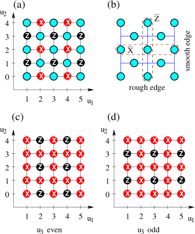
Figure 1: (color online) (a) Measurement pattern on the first and last slice of ${\cal{C}}$, for $l=5$. The resulting state is in the code space of the planar code. (The unmeasured qubits are displayed as shaded circles.) (b) Lattice for the planar code. (c)/(d) Measurement pattern for even and odd inner slices.

Before we consider errors, let us discuss the effect of this measurement pattern on a perfect cluster state. Consider some fixed outcomes $\{x_{u}\}$, $\{z_{u}\}$ of local measurements and let $|\psi\rangle_{LR}$ be the reduced state of the unmeasured qubits $L$ and $R$. We will now show that $|\psi\rangle_{LR}$ is, modulo local unitaries, an encoded Bell pair, with each qubit encoded by the planar code Kit2 , the planar counterpart of the toric code Kit1 . The initial cluster state obeys eigenvalue equations $K_{u}|\phi\rangle_{\cal{C}}=|\phi\rangle_{\cal{C}}$. This implies for the reduced state

$$Z_{P,u}|\psi\rangle_{LR}=\lambda_{P,u}|\psi\rangle_{LR},\;\;\forall\,\,u=(e,e,1),$$ (7)

where $Z_{P,u}=\bigotimes_{v\in\operatorname*{\mathop{\mathrm{neigh}}}(u)\cap L}Z_{v}$ is a plaquette ($z$-type) stabilizer operator for the planar code Kit2 . The eigenvalue $\lambda_{P,u}$ depends upon the measurements outcomes as $\lambda_{P,u}=x_{u}z_{(u_{1},u_{2},2)}$. Note that in the planar code the qubits live on the edges of a lattice rather than on its vertices. The planar code lattice is distinct from the cluster lattice ${\cal{C}}$; see Figs. 1,2.

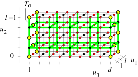
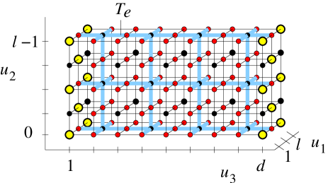
Figure 2: (color online) The measurement pattern on the cluster ${\cal{C}}$. The sublattices $T_{e}$ and $T_{o}$ are displayed (thick lines). For reference, the cluster lattice is also shown (thin lines) and the axis labeling shows the cluster coordinates. Cluster qubits measured in the $Z$-basis (on the sites of $T_{o}$ and $T_{e}$) are displayed in black, and qubits measured in the $X$-basis (on the edges of $T_{o}$ and $T_{e}$) are displayed in gray (red). The large circles to left and to the right denote the unmeasured qubits which form the encoded Bell pair. The measurement pattern has a bcc symmetry.

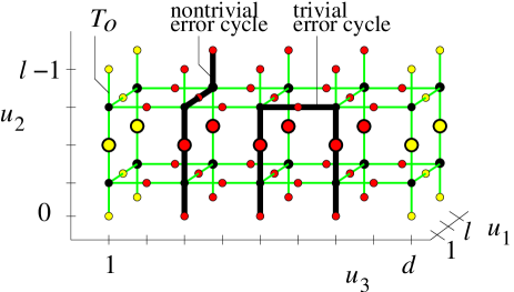
Figure 3: (color online) A homologically nontrivial and a homologically trivial error cycle on the lattice $T_{o}$. The nontrivial error cycle stretches from one rough face to the opposite one while the trivial error has both ends on the same face. Only the qubits belonging to $T_{o}$ are shown and the qubits important for establishing the $\overline{X}_{A}\overline{X}_{B}$-correlation are displayed enlarged.

From the equation $\prod_{v\in\operatorname*{\mathop{\mathrm{neigh}}}(u)}K_{v}\,|\phi\rangle_{\cal{C}}=|\phi\rangle_{\cal{C}}$, for $u=(o,o,1)$, we obtain

$$X_{S,u}|\psi\rangle_{LR}=\lambda_{S,u}|\psi\rangle_{LR},\;\;\forall\,\,u=(o,o,1),$$ (8)

where $X_{S,u}=\bigotimes_{v\in\operatorname*{\mathop{\mathrm{neigh}}}(u)\cap L}X_{v}$ coincides with a site ($x$-type) stabilizer operator for the planar code Kit2 , and $\lambda_{S,u}=x_{(u_{1},u_{2},2)}z_{u}\prod_{v\in\operatorname*{\mathop{\mathrm{neigh}}}_{o}(u)}z_{v}$, where $\operatorname*{\mathop{\mathrm{neigh}}}_{o}$ refers to a neighborhood relation on the sublattice $T_{o}$. The code stabilizer operators in Eq. (7) and (8) are algebraically independent. There are $(l^{2}-1)/2$ code stabilizer generators for $(l^{2}+1)/2$ unmeasured qubits, such that there exists one encoded qubit on $L$. By direct analogy, there is also one encoded qubit located on $R$.

Next, we show that $|\psi\rangle_{LR}$ is an eigenstate of $\overline{X}_{L}\overline{X}_{R}$ and $\overline{Z}_{L}\overline{Z}_{R}$, where $\overline{X}$ and $\overline{Z}$ are the encoded Pauli operators $X$ and $Z$, respectively, i.e. $|\psi\rangle_{LR}$ is an encoded Bell pair. The encoded Pauli operators Kit2 on $L$ and $R$ are $\overline{X}_{L[R]}=\bigotimes\limits_{u_{1}\,\,\text{odd}}X_{(u_{1},u_{2},1[d])}$ for any even $u_{2}$, and $\overline{Z}_{L[R]}=\bigotimes\limits_{u_{2}\,\,\text{even}}Z_{(u_{1},u_{2},1[d])}$ for any odd $u_{1}$. To derive the Bell-correlations of $|\psi\rangle_{LR}$ let us introduce 2D slices

$$\begin{array}[]{rcl}T_{\scriptscriptstyle XX}^{(u_{2})}&=&\{u=(o,u_{2},o)\in{\cal C}\}\subset T_{o},\\ T_{\scriptscriptstyle ZZ}^{(u_{1})}&=&\{u=(u_{1},e,e)\in{\cal C}\}\subset T_{e}.\\ \end{array}$$

The eigenvalue equation $\prod_{v\in T_{\scriptscriptstyle XX}^{(u_{2})}}K_{v}\,|\phi\rangle_{\cal{C}}=|\phi\rangle_{\cal{C}}$ with even $u_{2}$ implies for the reduced state

$$\overline{X}_{L}\overline{X}_{R}\,|\psi\rangle_{LR}=\lambda_{XX}\,|\psi\rangle_{LR},$$ (9)

with $\lambda_{XX}=\prod_{v\in T_{\scriptscriptstyle XX}^{(u_{2}+1)}\cup T_{\scriptscriptstyle XX}^{(u_{2}-1)}}z_{v}\prod_{v\in T_{\scriptscriptstyle XX}^{(u_{2})}\backslash(L\cup R)}x_{v}.$ Here and thereafter it is understood that $x_{u}=z_{u}=1$ for all $u\not\in{\cal{C}}$. Similarly, from $|\phi\rangle_{\cal{C}}=\prod_{v\in T_{\scriptscriptstyle ZZ}^{(u_{1})}}K_{v}\,|\phi\rangle_{\cal{C}}$, for $u_{1}$ odd, we obtain for the reduced state

$$\overline{Z}_{L}\overline{Z}_{R}\,|\psi\rangle_{LR}=\lambda_{ZZ}\,|\psi\rangle_{LR},$$ (10)

with $\lambda_{ZZ}=\prod_{v\in T_{\scriptscriptstyle ZZ}^{(u_{1}+1)}\cup T_{\scriptscriptstyle ZZ}^{(u_{1}-1)}}z_{v}\prod_{v\in T_{\scriptscriptstyle ZZ}^{(u_{1})}}x_{v}$. Thus the eigenvalue Eqs. (7-10) show that the measurement pattern of Eq. (6) projects the initial perfect cluster state into a state equivalent under local unitaries to the Bell pair, with each qubit encoded by the planar code.

It is crucial that the measurement outcomes $\{z_{u}\}$ and $\{x_{v}\}$ are not completely independent. Indeed, for any vertex $u\in T_{o}$ with $1<u_{3}<d$ the eigenvalue equation $\prod_{v\in\operatorname*{\mathop{\mathrm{neigh}}}(u)}K_{v}\,|\phi\rangle_{\cal{C}}=|\phi\rangle_{{\cal C}}$ implies the constraint

$$\prod_{v\in\operatorname*{\mathop{\mathrm{neigh}}}(u)}x_{v}\cdot\prod_{w\in\operatorname*{\mathop{\mathrm{neigh}}}_{o}(u)}z_{w}=1.$$ (11)

Analogously, for any vertex $u\in T_{e}$ one has a constraint

$$\prod_{v\in\operatorname*{\mathop{\mathrm{neigh}}}(u)}x_{v}\cdot\prod_{w\in\operatorname*{\mathop{\mathrm{neigh}}}_{e}(u)}z_{w}=1,$$ (12)

where $\operatorname*{\mathop{\mathrm{neigh}}}_{e}$ refers to a neighborhood relation on the lattice $T_{e}$. Thus there exists one syndrome bit for each vertex of $T_{e}$ and $T_{o}$, (with exception for the vertices of $T_{o}$ with $u_{3}=1$ or $u_{3}=d$).

What are the errors detected by these syndrome bits? Since we have only $Z$-errors (for generalization, see remark 1), only the $X$-measurements are affected by them. Each $X$-measured qubit is either on an edge of $T_{o}$ or $T_{e}$. Thus, we can identify the locations of the elementary errors with $E(T_{o})$ and $E(T_{e})$. From the equations Eq. (11,12), each error located on an edge creates a syndrome at its end vertices.

Let us briefly compare with TCDS . Therein, independent local $X$-and $Z$-errors were considered for storage whose correction runs completely independently. The $X$-errors in this model correspond to our $Z$-errors on qubits in $E(T_{e})$, and the $Z$-storage errors to our $Z$-errors on qubits in $E(T_{o})$, if the $X-$ and $Z-$error correction phases in TCDS are pictured as alternating in time.

The syndrome information provided by Eqs. (11,12) is not yet complete. There are two important issues to be addressed: (i) There are no syndrome bits at the vertices of $T_{o}$ with $u_{3}=1$ or $u_{3}=d$; (ii) Edges of $T_{e}$ with $u_{3}=1$ or $u_{3}=d$ have only one end vertex, so errors that occur on these edges create only one syndrome bit. Concerning (i), to get the missing syndrome bits we will measure eigenvalues $\lambda_{P,u}$ and $\lambda_{S,u}$ for the plaquette and the site stabilizer operators living on the faces $A$ and $B$, see Eqs. (7,8). Such measurements are local operations within $A$ or within $B$, so they can not increase entanglement between $A$ and $B$. For any $u=(o,o,1)$ or $u=(o,o,d)$ it follows from Eq. (8) that

$$\begin{array}[]{rclr}\displaystyle{\lambda_{S,u}\,x_{(u_{1},u_{2},2)}\,z_{u}\prod_{v\in\operatorname*{\mathop{\mathrm{neigh}}}_{o}(u)}z_{v}}&=&1,&\mbox{for }u_{3}=1,\\ \displaystyle{\lambda_{S,u}\,x_{(u_{1},u_{2},d-1)}\,z_{u}\prod_{v\in\operatorname*{\mathop{\mathrm{neigh}}}_{o}(u)}z_{v}}&=&1,&\mbox{for }u_{3}=d.\end{array}$$ (13)

For any vertex $u=(o,o,1)$ or $u=(o,o,d)$ there are several edges of the lattice $T_{o}$ incident to $u$. It is easy to see that a single $Z$-error that occurs on any of these edges changes a sign in Eqs. (13). Thus, these two constraints yield the syndrome bits living at the vertices $u=(o,o,1)$ and $u=(o,o,d)$, so the issue (i) is addressed. Concerning (ii), we make use of Eq. (7) and obtain

$$\begin{array}[]{rclr}\lambda_{P,u}\,x_{u}z_{(u_{1},u_{2},2)}&=&1,&\mbox{for any }u=(e,e,1),\vspace{2mm}\\ \lambda_{P,u}\,x_{u}z_{(u_{1},u_{2},d-1)}&=&1,&\mbox{for any }u=(e,e,d).\end{array}$$ (14)

Since we have only $Z$-errors, the eigenvalues $\lambda_{P,u}$ and the outcomes $z_{(u_{1},u_{2},2)}$, $z_{(u_{1},u_{2},d-1)}$ are not affected by errors. Thus the syndrome bits Eqs. (14) are equal to $-1$ iff an error has occurred on the edge $u=(e,e,1)$ or $u=(e,e,d)$ of the lattice $T_{e}$. Since each of these errors shows itself in a corresponding syndrome bit which is not affected by any other error, we can reliably identify these errors. This is equivalent to actively correcting them with unit success probability. We can therefore assume in the subsequent analysis that no errors occur on the edges $(e,e,1)$ and $(e,e,d)$, which concludes the discussion of the issue (ii).

As in Kit1 , we define an error chain ${\cal{E}}$ as a collection of edges where an elementary error has occurred. Each of the two lattices $T_{e}$ and $T_{o}$ has its own error chain. An error chain ${\cal{E}}$ shows a syndrome only at its boundary $\partial({\cal{E}})$, and errors with the same boundary thus have the same syndrome. One may identify an error ${\cal{E}}$ only modulo a cycle $D$, ${\cal{E}}^{\prime}={\cal{E}}+D$, with $\partial(D)=0$.

There are homologically trivial and nontrivial cycles. A cycle $D$ is trivial if it is a closed loop in $T_{o}$ ($T_{e}$), and homologically nontrivial if it stretches from one rough face in $T_{o}$ ($T_{e}$) to another. A rough face here is the 2D analogue of a rough edge on a planar code Kit2 . The rough faces of $T_{o}$ are on the upper and lower side of ${\cal{C}}$, and the rough faces of $T_{e}$ are on the front and back of ${\cal{C}}$ (recall that no errors occur on the left and right rough faces of $T_{e}$).

Let us now study the effect of error cycles on the identification of the state $|\psi\rangle_{LR}$ from the measurement outcomes. We only discuss the error chains on $T_{o}$ here, which potentially affect the eigenvalue Eq. (9). The discussion of the error chains in $T_{e}$—which disturb the $\overline{Z}_{L}\overline{Z}_{R}$-correlations—is analogous. An individual qubit error on $v\in{\cal{C}}$ will modify the $\overline{X}_{L}\overline{X}_{R}$ correlation of $|\psi\rangle_{LR}$ if it either affects $\overline{X}_{L}$, $\overline{X}_{R}$ or $\lambda_{XX}$. That happens if $v\in T_{XX}^{(u_{2})}$. Now, the vertices in $T_{XX}^{(u_{2})}$ correspond to edges in $T_{o}$. If an error cycle $D$ in $T_{o}$ is homologically trivial, it intersects $T_{XX}^{(u_{2})}$ in an even number of vertices; see Fig. 3. This has no effect on the eigenvalue Eq. (9). However, if the cycle is homologically nontrivial, i.e. if it stretches between the upper and lower face of ${\cal{C}}$, then it intersects $T_{XX}^{(u_{2})}$ in an odd number of vertices. This does modify the eigenvalue Eq. (9) by a sign factor of $(-1)$ on the l.h.s., which leads to a logical error. Therefore, for large system size, we require the probability of misinterpreting the syndrome by a nontrivial cycle to be negligible TCDS :

$$\sum_{\cal{E}}\text{prob}({\cal{E}})\sum_{D\;\text{nontrivial}}\text{prob}({\cal{E}}+D|\,{\cal{E}})\,\approx\,0.$$ (15)

We have now traced back the problem of reconstructing an encoded Bell pair $|\psi\rangle_{LR}$ to the same setting that was found in TCDS to describe fault-tolerant data storage with the toric code. Via the measurement pattern Eq. (6), we may introduce two lattices $T_{o}$, $T_{e}$ such that 1) Syndrome bits are located on the vertices of these lattices, 2) Independent errors live on the edges and show a syndrome on their boundary, 3) Only the homologically nontrivial cycles give rise to a logical error. This error model can be mapped onto a random plaquette $Z_{2}$-gauge field theory in 3 dimensions TCDS ; WHP which undergoes a phase transition between an ordered low temperature and a disordered high temperature phase. In the limit of $l,d\longrightarrow\infty$, full error-correction is possible in the low temperature phase.

In our setting, the error probabilities for all edges are equal to $p$. For this case the critical error probability has been computed numerically in a lattice simulation PT_Nishimori , $p_{c}=0.033\pm 0.001$. This value corresponds, via Eq. (5), to $T_{c}=(0.296\pm 0.003)\Delta$.

Remarks: 1) The error model equivalent to Eq. (3), i.e. $Z$-errors only, is very restricted. We have a physical motivation for this model, but we would like to point out that the very strong assumptions we have made about the noise are not crucial to our result of the threshold error rate being non-zero. One may, for example, generalize the error model from a dephasing channel to a depolarizing channel, with $p_{x}=p_{y}=p_{z}=p^{\prime}/3$. Then, two changes need to be addressed, those in the bulk and those on the faces $L$ and $R$. Concerning the faces, the errors on the rough faces to the left and right of $T_{e}$ can no longer be unambiguously identified by measurements of the code stabilizer (14), which raises the question of whether—for depolarizing errors—it may be these surface errors that set the threshold for long-range entanglement. This is not the case. To see this, note that two slices of 2D cluster states may be attached to the left and right of ${\cal{C}}$, at $u_{3}=0,-1$ and $u_{3}=d+1,d+2$. The required operations are assumed to be perfect. They do not change the localizable entanglement between the left and right side of the cluster ${\cal{C}}$ because they act locally on the slices $-1..1$ and $d..d+2$, respectively. The subsets $A$ and $B$ of spins are re-located to the slices $-1$ and $d+2$, with the corresponding changes in the measurement pattern. The effect of this procedure is that the leftmost and rightmost slice of the enlarged cluster are error-free , and only the bulk errors matter.

Concerning the bulk, note that the cluster qubits measured in $Z$-basis serve no purpose and may be left out from the beginning. Then, the considered lattice for the initial cluster state has a bcc symmetry and double spacing. The lattices $T_{o}$, $T_{e}$ remain unchanged. Further, $X$-errors are absorbed in the $X$-measurements and $Y$-errors act like $Z$-errors, such that we still map to the original $\mathbb{Z}_{2}$ gauge model TCDS at the Nishimori line. The threshold for local depolarizing channels applied to this configuration is thus $p^{\prime}_{c}=3/2\,p_{c}=4.9\%$. In addition, numerical simulations performed for the initial simple cubic cluster and depolarizing channel yield an estimate of the critical error probability of $p^{\prime\prime}_{c}=1.4\%$.
2) Finite size effects. We carried out numerical simulations of error correction on an $l\times l\times d$ lattice with periodic boundary conditions (as opposed to the open boundary conditions of the planar codes within the cluster state). For differing error rates below the threshold value of $2.9\%$ WHP , we found good agreement for the fidelity $F$ between the perfect and the error-corrected encoded Bell state with the model $F\sim\exp(-dk_{1}\exp(-lk_{2}))$. Some data is shown in Fig. 4 corresponding to a $Z$-error rate of $1.0\%$. Provided that planar codes and toric codes have similar behavior away from threshold, our simulations suggest that, in order to achieve constant fidelity, the length $l$ specifying the surface code need only scale logarithmically with the distance $d$.
3) For even $d$, the construction presented above can be used to mediate an encoded conditional $Z$-gate on distant encoded qubits located on slices $1$ and $d$.

Figure 4: This figure plots data for simulations of error correction on an $L\times L\times d_{\text{toric}}$ lattice, with periodic boundary conditions in the first two directions, for various $L$ and $d_{\text{toric}}$ ($d=2d_{\text{toric}}+1$, $l=2L$). The error rate is $p=0.01$. The logs are base $e$. Two standard deviations above and below the computed values (as given by statistical noise due to the sample sizes) are shown by the error bars. The solid lines each have slope one, and they are spaced equally apart. This lends good support to the model of fidelity $F\sim\exp(-dk_{1}\exp(-lk_{2}))$ for error rates below threshold.

III Upper bound

In this section we analyze the high-temperature behavior of thermal cluster states and find an upper bound on the critical temperature $T_{c}$. Our analysis is based on the isomorphism between cluster states and the so-called Valence Bond Solids (VBS) pointed out by Verstraete and Cirac in Verstraete_Cirac_VBS which can easily be generalized to a finite temperature.

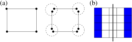
Figure 5: (color online) (a) Correspondence between physical and virtual qubits. Domains are shown by dashed lines. (b) A bipartite cut of a cubic lattice. The regions $A$ and $B$ are highlighted.

With each physical qubit $u\in{\cal C}$ we associate a domain $u.*$ of $d(u)$ virtual qubits, where $d(u)=|\operatorname*{\mathop{\mathrm{neigh}}}(u)|$ is the number of nearest neighbors of $u$ (see Fig. 5 (a)). Let us label virtual qubits from a domain $u.*$ as $u.v$, $v\in\operatorname*{\mathop{\mathrm{neigh}}}(u)$. Denote $E$ to be the set of edges of the lattice ${\cal C}$ and define a thermal VBS state $\rho_{\scriptscriptstyle V\!BS}$ as

$$\rho_{\scriptscriptstyle V\!BS}=\prod_{e=(u,v)\in E}\frac{1}{4}\left(I+\omega_{e}X_{u.v}Z_{v.u}\right)\left(I+\omega_{e}Z_{u.v}X_{v.u}\right).$$ (16)

Here $\{\omega_{e}\}$ are arbitrary weights such that $0\leq\omega_{e}\leq 1$. It should be emphasized that $\rho_{\scriptscriptstyle V\!BS}$ is a state of virtual qubits rather than physical ones. Our goal is to convert $\rho_{\scriptscriptstyle V\!BS}$ into $\rho_{\scriptscriptstyle CS}$ by local transformations mapping a domain $u.*$ into a single qubit $u\in{\cal C}$. The following theorem is a straightforward generalization of the Verstraete and Cirac construction (here we put $\Delta/2=1$).

Theorem 1.

Let $\rho_{\scriptscriptstyle CS}$ be a thermal cluster state on the 3D cubic lattice ${\cal C}$ at a temperature $T\equiv\beta^{-1}$. Consider a thermal VBS state $\rho_{\scriptscriptstyle V\!BS}$ as in Eq. (16) such that the weights $\omega_{e}$ satisfy

$$\prod_{v\in\operatorname*{\mathop{\mathrm{neigh}}}{(u)}}\omega_{(u,v)}\,\geq\tanh{(\beta)}\quad\mbox{for each}\quad u\in{\cal C}.$$ (17)

Then $\rho_{\scriptscriptstyle V\!BS}$ can be converted into $\rho_{\scriptscriptstyle CS}$ by applying a completely positive transformation ${\cal{W}}_{u}$ to each domain $u.*$,

$$\rho_{\scriptscriptstyle CS}={\cal{W}}(\rho_{\scriptscriptstyle V\!BS}),\quad{\cal{W}}=\bigotimes_{u\in{\cal C}}{\cal{W}}_{u}.$$ (18)

Let us first discuss the consequences of this theorem. Note that each edge $e\in E$ of $\rho_{\scriptscriptstyle V\!BS}$ carries a two-qubit state

$$\rho_{e}=\frac{1}{4}(I+\omega_{e}X_{1}Z_{2})(I+\omega_{e}Z_{1}X_{2}).$$ (19)

The Peres-Horodecki partial transpose criterion Peres_PPT ; Horodecki_PPT tells us that $\rho_{e}$ is separable if and only if $\omega_{e}\leq\sqrt{2}-1$. Consider a bipartite cut of the lattice by a hyperplane of codimension 1 (see Fig. 5 (b)). We can satisfy Eq. (17) by setting $\omega_{e}=\tanh{(\beta)}$ for all edges crossing the cut and setting $\omega_{e}=1$ for all other edges. Clearly, the state $\rho_{\scriptscriptstyle V\!BS}$ is bi-separable whenever $\tanh{(\beta)}\leq\sqrt{2}-1$. But bi-separability of $\rho_{\scriptscriptstyle V\!BS}$ implies bi-separability of $\rho_{\scriptscriptstyle CS}$. We conclude that the localizable entanglement between the regions $A$ and $B$ is zero whenever $\tanh{(\beta)}\leq\sqrt{2}-1$, which yields the upper bound on $T_{c}$ presented earlier.

Remarks: We can also satisfy Eq. (17) by setting $\omega_{e}=\omega$ for all $e\in E$, with $\omega^{6}=\tanh{(\beta)}$. This choice demonstrates that $\rho_{\scriptscriptstyle CS}$ is completely separable for $\tanh{(\beta)}<(\sqrt{2}-1)^{6}$ (that is $T\approx 200$). It reproduces the upper bound MacE of Dür and Briegel on the separability threshold error rate for cluster states.

In the remainder of this section we prove Theorem 1. Consider an algebra ${\cal A}_{u}$ of operators acting on some particular domain $u.*$. It is generated by the Pauli operators $Z_{u.v}$ and $X_{u.v}$ with $v\in\operatorname*{\mathop{\mathrm{neigh}}}{(u)}$. The transformation ${\cal{W}}_{u}$ maps ${\cal A}_{u}$ into the one-qubit algebra generated by the Pauli operators $Z_{u}$ and $X_{u}$. First, we choose

$${\cal{W}}_{u}(\eta)=W_{u}^{\dagger}\,\eta\,W_{u},\quad W_{u}=|0^{\otimes d(u)}\rangle\langle 0|+|1^{\otimes d(u)}\rangle\langle 1|.$$

One can easily check that

$$W_{u}^{\dagger}Z_{u.v}=Z_{u}W_{u}^{\dagger}\quad\mbox{and}\quad Z_{u.v}W_{u}=W_{u}Z_{u},$$ (20)

for any $v\in\operatorname*{\mathop{\mathrm{neigh}}}{(u)}$. As for commutation relations between $W_{u}$ and $X_{u.v}$ one has

$$\begin{array}[]{rcl}W_{u}^{\dagger}\,\left(\prod_{v\in\operatorname*{\mathop{\mathrm{neigh}}}{(u)}}X_{u.v}\right)\,W_{u}&=&X_{u},\\ W_{u}^{\dagger}\,\left(\prod_{v\in S}X_{u.v}\right)\,W_{u}&=&0,\end{array}$$ (21)

for any non-empty proper subset $S\subset\operatorname*{\mathop{\mathrm{neigh}}}{(u)}$. Taking ${\cal{W}}=\bigotimes_{u\in{\cal C}}{\cal{W}}_{u}$ and using Eqs. (20), (21) one can easily get

$${\cal{W}}(\rho_{\scriptscriptstyle V\!BS})=\frac{1}{4^{|E|}}\prod_{u\in{\cal C}}\left(I+\eta_{u}K_{u}\right),\quad\eta_{u}=\prod_{v\in\operatorname*{\mathop{\mathrm{neigh}}}{(u)}}\omega_{(u,v)}.$$ (22)

We can regard the state in Eq. (22) as a thermal cluster state with a local temperature $\tanh{(\beta_{u})}\equiv\eta_{u}$ depending upon $u$. The inequality of Eq. (17) implies that $\beta_{u}\geq\beta$ for all $u$. To achieve a uniform temperature distribution $\beta_{u}=\beta$ one can intentionally apply local $Z$-errors with properly chosen probabilities.

IV Conclusion

Thermal cluster states in three dimensions exhibit a transition from infinite to finite entanglement length at a non-zero transition temperature $T_{c}$. We have given a lower and an upper bound to $T_{c}$, $0.3\,\Delta\leq T_{c}\leq 1.15\,\Delta$ ($\Delta=$ energy gap of the Hamiltonian). The reason for $T_{c}$ being non-zero is an intrinsic error-correction capability of 3D cluster states. We have devised an explicit measurement pattern that establishes a connection between cluster states and surface codes. Using this, we have described how to create a Bell state of far separated encoded qubits in the low-temperature regime $T<0.3\,\Delta$, making the entanglement contained in the initial thermal state accessible for quantum communication and computation.

References

• (1) J.S. Bell, Physics 1, 195 (1964).
• (2) A. Aspect, P. Grangier and G. Roger, Phys. Rev. Lett. 47, 460 (1981).
• (3) E. SchrΓΆdinger, Naturwissenschaften 23, 807-812, 823-828, 844-849 (1935).
• (4) H.J. Briegel, W. DΓΌr, J.I. Cirac, and P.Zoller, Phys. Rev. Lett. 81, 5932 (1998).
• (5) F. Verstraete, M. Popp and J.I. Cirac, Phys. Rev. Lett. 92, 027901 (2004).
• (6) D. Aharonov, quant-ph/9910081 (1999).
• (7) F. Verstraete, M.A. MartΓ­n-Delgado, J.I. Cirac, Phys. Rev. Lett. 92, 087201 (2004).
• (8) I. Affleck, T. Kennedy, E.H.Β Lieb, and H.Β Tasaki, Commun. Math. Phys. 115, 477 (1998).
• (9) J.K. Pachos and M.B. Plenio, Phys. Rev. Lett. 93, 056402 (2004).
• (10) A. Kay et al., quant-ph/0407121 (2004).
• (11) H.J. Briegel and R. Raussendorf, Phys. Rev. Lett. 86, 910 (2001).
• (12) E. Dennis, A. Kitaev, A. Landahl, and J. Preskill, quant-ph/0110143 (2001).
• (13) S. Bravyi, A. Kitaev, quant-ph/9811052 (1998).
• (14) A. Kitaev, quant-ph/9707021 (1997).
• (15) C. Wang, J. Harrington and J. Preskill, Annals Phys. 303, 31 (2003), quant-ph/0207088 (2002).
• (16) T. Ohno, G. Arakawa, I. Ichinose and T. Matsui, quant-ph/0401101 (2004).
• (17) F. Verstraete and J.I. Cirac, quant-ph/0311130 (2003).
• (18) A. Peres, Phys. Rev. Lett. 77, 1413 (1996).
• (19) M. Horodecki, P. Horodecki, and R. Horodecki,
Phys.Β Lett.Β A 223, 1 (1996).
• (20) W. DΓΌr and H.J. Briegel, Phys. Rev. Lett. 92, 180403 (2004).